Article

Sensitivity Analysis of Krasovskii Passivity-Based Controllers †

Department of Automation, Technical University of Cluj-Napoca, Str. G. Bariţiu Nr. 26-28, 400027 Cluj-Napoca, Romania
*
Authors to whom correspondence should be addressed.
This paper is an extended version of our paper published in Proceedings of the 2022 IEEE International Conference on Automation, Quality and Testing, Robotics (AQTR), Cluj-Napoca, Romania, 19–21 May 2022; https://doi.org/10.1109/AQTR55203.2022.9802070.
These authors contributed equally to this work.
Mathematics 2022, 10(20), 3750; https://doi.org/10.3390/math10203750
Submission received: 25 August 2022 / Revised: 18 September 2022 / Accepted: 30 September 2022 / Published: 12 October 2022
(This article belongs to the Section Engineering Mathematics)

Abstract

:
In the domain of passivity theory, there were major contributions in the last decade, the most recent notion of passivity being the so-called Krasovskii passivity. This framework offers the possibility of designing a controller which ensures the passivity of the resulting closed-loop system. The current paper proposes a solution to design the parameters of Krasovskii passivity-based controllers (K-PBCs) in order to ensure small sensitivity of the closed-loop systems. As such, after the initial construction of the passivity output, the controller parameters are designed in order to impose the dominant eigenvalues of the Jacobian of the resulting closed-loop system with the smallest deviation around the given forced equilibrium point which is, additionally, smaller than a prescribed stability margin. The resulting optimization problem is non-convex by nature, and a metaheuristic approach is proposed to design these parameters. Moreover, in order to impose an extra set of performances, the control system contains an outer loop where dynamical path planning is used to impose the additional requirements. All mentioned results are developed for processes modeled as bilinear systems. In order to illustrate the proposed control method, a numerical example consisting of a single-ended primary inductor DC-DC converter (SEPIC) process is presented.

1. Introduction

1.1. Literature Review

Passivity theory was developed fifty years ago when the notion of dissipative systems was introduced in [1], and it describes an input–output property of a nonlinear system, having the interpretation of the difference between the stored energy in the system and the supply rate. In [2], the notion of dissipative systems and the special case of passive systems are underlined as a tool to study the input–output relation of a nonlinear system. L 2 -gain theory and passivity are presented in [3] in a unified manner for nonlinear systems described using state-space models. The book also offers a compact treatment of well-known small-gain and passivity theorems for nonlinear systems described using input–output maps. A monograph that deals with passivity-based tools for problems such as robust control, fault tolerant control, or decentralized control for industrial processes is in [4].
Starting from the idea of incremental stability of nonlinear systems, the notion of incremental passivity has been used in [5], presenting a method to construct an output feedback controller which manages to achieve incremental passivity property for a special class of systems, nonlinear by nature. In addition, the paper [6] extends the incremental passivity for the case of nonlinear switched systems, studying the global output regulation for this class of systems. Additionally, this paper manages to extend these notions for systems whose subsystems are not required to be incrementally passive. Recently, the classical passivity notion has been extended in [7,8] to the notion of differential passivity, where, besides the nonlinear system itself, the variational system was also considered, resulting in a prolonged system. Differential passivity is a property of such a prolonged system, general geometric conditions for gradient and Brayston–Moser systems being available in the aforementioned papers. Another class of systems discussed in the topic of passivity-based control is the class of port-Hamiltonian systems. A passivity approach for the case of port-Hamiltonian systems for multi-agent formation control and velocity tracking is proposed in [9]. Another notion that fills the gap between the classical passivity and incremental passivity is that of shifted passivity, which can be seen as a generalized version of passivity for other nontrivial equilibrium points [10].
The idea of Krasovskii passivity was introduced for the first time in [11] and proposes a method to construct the storage function using Krasovskii’s method to construct Lyapunov functions for stability study. In addition, a method to design a passivity-based controller (PBC) is presented in the previously mentioned paper. In [12], a set of relations between differential, incremental, shifted and Krasovskii passivity are established. In addition, a mechanism to design Krasovskii passivity-based controllers (K-PBCs) and shifted passivity-based controllers (S-PBCs) for a class of nonlinear systems is offered, the class of port-Hamiltonian systems being representative. A set of sufficient conditions for a bilinear system to be Krasovskii passive has been presented in [13], and in a similar manner, the set of conditions has been extended in [14] for nonlinear systems which can be bounded by a polytopic bilinear system. In [13,14], a cascade control structure with an inner K-PBC and an outer dynamical path-planning robust controller, was proposed. The problem of robust output regulation has been addressed using the passivity theory in [15] for the case of DC power networks where the considered loads are of type impedance, current or power.
The passivity-based control techniques can be extended to the case of switching systems. For the case of switched linear systems, the paper [16] presents a control design problem related to the determination of a switching strategy that renders a switched linear system passive. Moreover, for the case of linear systems, the positive real lemma plays an important role and links the passivity with the linear matrix inequalities framework, but it requires an extra assumption for the system to be controllable. This lemma has been recently developed in [17] and offers a mechanism to determine if an uncontrollable linear system is passive. In the same manner, the results available for controllable reciprocal systems have been extended for the uncontrollable case in [18].

1.2. Contributions and Paper Structure

As mentioned, the notion of Krasovskii passivity has been developed in the last five years and offers a mechanism to construct a passivity-based controller. However, none of the papers [11,12,13,14] present a method to design the parameters of K-PBCs, which represents the starting point of the current paper. In the recent conference paper [19], an ad hoc analysis to tune the previously mentioned parameters using a method similar with the classical root-locus was proposed. As such, the current journal paper presents an extensive method to find the sub-optimal values of the Krasovskii passivity-based controller parameters instead of the initially proposed isolated analysis. The key points of the paper are:
(i)
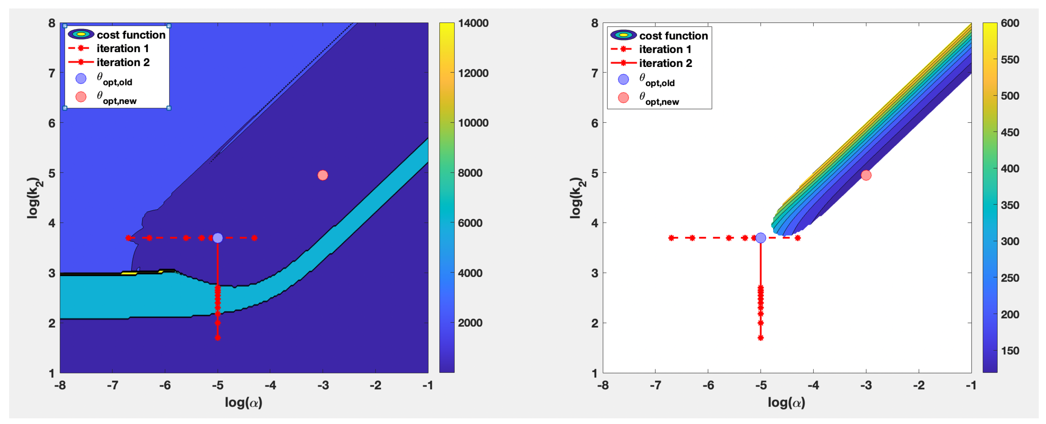
The ad hoc analysis proposed in [19], based on a trial and error methodology, is replaced with a more rigorous treatment using the sensitivity analysis of the resulting closed-loop system. To measure the sensitivity, we consider the length of the curve described by the dominant eigenvalue of the Jacobian of the closed-loop system.
(ii)
The length of the path of the aforementioned dominant eigenvalues can be used as a performance index which can be minimized in terms of K-PBC’s parameters, resulting in a non-convex optimization problem. In the current paper, there are two possibilities presented to formulate the optimization problem: one by minimizing only the sensitivity of the inner closed-loop system, and the latter by minimizing this sensitivity function with an extra constraint of having the inner dynamics at least twice as fast as the dominant dynamics imposed by the outer dynamical path planning.
(iii)
The two said optimization problems formulated in this journal paper are non-convex by nature. As such, a global optimization technique is required in order to find the sub-optimal value of the controller’s parameters. For the purpose of this paper, we developed a slightly modified version of the Artificial Bee Colony (ABC) algorithm [20], the main modification being in terms of stopping criteria and abandonment counters management, all modifications increasing the speed of the algorithm and avoiding the search in the unfeasible zone. Being a metaheurisitc approach for a non-convex optimization problem, only a sub-optimal value of these parameters can be guaranteed, but the exploration ability of the ABC algorithm leads to good results.
(iv)
Finally, in order to prove the efficiency of the proposed method, we present an end-to-end design approach for a nonideal DC-DC single-ended primary-inductor converter (SEPIC), starting from the method of constructing the passivity output, along with designing the outer dynamical path planning for the linearized system around a desired equilibrium point, and also the solution to the optimization problem regarding the sub-optimal choice of the K-PBC’s parameters. All results presented are obtained using the MATLAB-based toolbox initially described in [21] and extended in [13] for the nonlinear model.
The paper next contains the following sections: Section 2, which presents the main theoretical background for the Krasovskii passivity and for the robust control framework; Section 3, which illustrates the mechanism used to formulate the optimization problems which leads to the sub-optimal values of the controller parameters, along with the metaheuristic approach which manages to solve these non-convex problems; Section 4, which presents an end-to-end approach to design both the K-PBC controller and dynamic path planning alike from the proposed structure for a DC-DC SEPIC converter; Section 5, where a set of final remarks and a discussion based on the obtained results are emphasized, while Section 6 contains conclusions and future work.

1.3. Notations

We will use > ( ) 0 to denote that a symmetrical matrix Q = Q R n × n is positive (semi-)definite. For a vector x R n and a symmetrical and positive-definite matrix Q = Q > 0 R n × n , we define the norm · Q by x Q : = ( x Q x ) 1 / 2 .

2. Mathematical Background

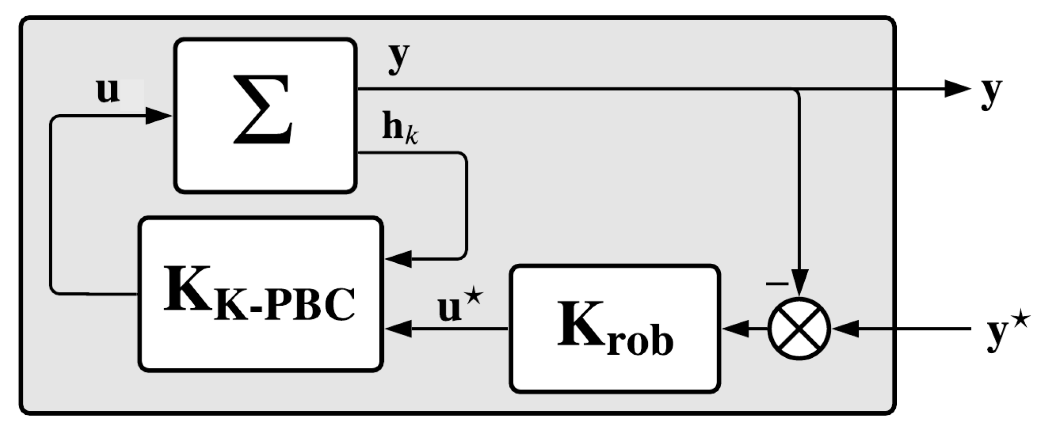
2.1. Krasovskii Passivity

The purpose of the current subsection is to briefly introduce the main notions regarding the passivity-based controller design procedure using Krasovskii’s method presented in several recent papers [11,12,13,14,19] in order to increase the readability of this journal paper. The proofs for all mentioned results can be founded in the above-mentioned papers. We start by describing the framework used to model the systems, namely the bilinear systems framework.
Definition 1.
A single-input and input-affine continuous-time nonlinear system ( Σ ) is called bilinear if it has the following input-to-state representation:
( Σ ) : x ˙ = f ( x , u ) A 0 x + b 0 + A 1 x + b 1 u ,
where u R is the input, x R n is the state vector, while A 0 , A 1 R n × n and b 0 , b 1 R n × 1 .
Definition 2.
A bilinear system ( Σ Δ ) is called uncertain if it has the state-space representation:
( Σ Δ ) : x ˙ = f Δ ( x , u ) A 0 + Δ A 0 x + b 0 + Δ b 0 + A 1 + Δ A 1 x + b 1 + Δ b 1 u ,
where Δ A 0 , Δ A 1 R n × n and Δ b 0 , Δ b 1 R n × 1 are the uncertainty matrices described by a set Δ.
Let us consider D x the reachable domain and D u the domain of the admissible inputs. The following assumption is mandatory: to each input u = u ¯ D u R corresponds at least one forced feasible equilibrium point of the bilinear nominal plant ( Σ ) , i.e., there exists x ¯ D x such that f ( x ¯ , u ¯ ) = 0 . The following notion of dissipative systems was introduced in [2]:
Definition 3.
A bilinear system (Σ) is dissipative with respect to a function ω : R n × R R , called the supply rate, if a storage function S : R n R + of class C 1 can be constructed such that:
S ( x ) x f ( x , u ) ω ( x , u ) , ( ) ( x , u ) R n × R .
However, as already proved in the previous work [13], in such classical approaches, the resulting passivity operator cannot be used in the construction of a controller. A solution to this issue consists in considering the extended system ( Σ e ) by augmenting the system ( Σ ) at the input with an extra integrator, as in [1]. As such, the new extended state vector can be written as x ˜ = [ x u ] R n + 1 , the new input being u d u . The Krasovskii method of constructing a Lyapunov function was used in [11] to introduce an extension of the passivity concept as follows:
Definition 4.
Let h K : R n × R R be the function which describes the passivity output variable. The nominal bilinear system (Σ) is said to be Krasovskii passive if its extended system ( Σ e ) is dissipative with respect to the supply rate:
ω K : R n + 1 × R R , ω K ( x ˜ , u d ) = u d · h K ( x ˜ ) ,
with a storage function:
S K : R n × R R + , S K ( x ˜ ) = 1 2 f ( x , u ) Q 2 , with Q = Q 0 .
Next, a set of sufficient conditions for an input-affine nonlinear system to be Krasovskii passive is described. Starting from the results presented in [11], a set of sufficient conditions to construct an output such that the system is Krasovskii passive has been proposed in [13] for the case of bilinear systems:
Theorem 1.
The nominal system ( Σ ) is Krasovskii passive with the supply-rate ω K : R n × R R , ω K ( x ˜ , u d ) = u d · h K ( x ˜ ) , where the output variable h K can be expressed as:
h K ( x ˜ ) h K ( x , u ) = x A 1 + b 1 · Q · f ( x , u ) ,
and with the storage function:
S K ( x ˜ ) S K ( x , u ) = 1 2 f ( x , u ) Q 2 ,
if there exists a matrix Q R n × n , Q = Q 0 , which satisfies the following condition:
Q A 0 + A 0 Q + Q A 1 + A 1 Q u 0 , u D u .
Now, using the convexity of the LMI problem (6), the following theorem can be used in order to reduce the order of this LMI problem.
Theorem 2.
Considering a bounded admissible input set D u = [ u ̲ , u ¯ ] , the nominal system ( Σ ) is Krasovskii passive with the supply-rate ω K : R n × R R , ω K ( x ˜ , u d ) = u d · h K ( x ˜ ) , where the output variable h K can be expressed as:
h K ( x ˜ ) h K ( x , u ) = x A 1 + b 1 · Q · f ( x , u ) ,
and with the storage function:
S K ( x ˜ ) S K ( x , u ) = 1 2 f ( x , u ) Q 2 ,
if there exists a matrix Q R n × n , Q = Q 0 , which satisfies the following conditions:
Q A 0 + A 0 Q + Q A 1 + A 1 Q u ̲ 0 ; Q A 0 + A 0 Q + Q A 1 + A 1 Q u ¯ 0 .
To design a passivity-based controller using the Krasovskii’s methodology to construct Lyapunov functions, a SISO proportional–integrative (PI) structure can be considered, as in [11,13]:
( Σ c ) : y c = x ˙ c = k 1 ( k 2 x c u c ) f c ( x c , u c ) ,
where x c is the state vector, u c and y c are the input and output signals, respectively, and terms k 1 , k 2 R + are controller parameters. According to [11], for each combination of positive values chosen for the parameters k 1 and k 2 , a controller having the structure as in (10) is Krasovskii passive with respect to the supply-rate ω K , c ( y c , u c ) = y c · u c according to the storage function:
S K , c : R R + , S K , c = 1 2 k 2 x c 2 .
The lower linear fractional transform (LLFT) interconnection between ( Σ e ) and ( Σ c ) is:
u d u c = 0 1 1 0 h K y c + 0 u ,
where u is the reference of the closed-loop system. The following theorem extended from [11] characterizes the closed-loop system with input u and output h K :
Theorem 3.
The closed-loop system obtained using the extended system ( Σ e ) , which satisfies the conditions of Theorem 1 for a matrix Q R n × n , Q = Q > 0 , with a feasible forced equilibrium point ( x ¯ , u ¯ ) D x × D u , having an LLFT interconnection with the controller given by ( Σ c ) , with the states x c = u u , is dissipative with respect to the supply rate ω o ( u d , u ) = u d · u with the storage function:
S o ( x , u , x c ) = 1 2 f ( x , u ) Q 2 + 1 2 K 2 2 x c .
Remark 1.
If the integrator used to augment the bilinear system in order to obtain the extended form ( Σ e ) is inserted into the K-PBC, the state-space representation of the controller becomes:
( Σ K P B C ) : x ˙ c = k 1 k 2 x c k 1 h K ( x ˜ ) + k 1 k 2 u ; y c = x c .

2.2. Dynamic Path-Planning

As stated before, the closed-loop system resulting from the LLFT interconnection between the bilinear system ( Σ ) and the Krasovskii passivity-based controller ( Σ K P B C ) ensures the stability of the nonlinear system without imposing the desired steady-state performance. As such, the outer controller is used as a dynamic path planning which computes the trajectory u based on the error signal ε = y y , where y is the reference signal and y is the measured output of the system ( Σ ) , as in Figure 1. Moreover, the uncertainty part of the bilinear system ( Σ Δ ) must also be resolved using the outer dynamic path planning. As such, the robust control framework (RCF) is a good choice for the purpose of the proposed method.
Although the RCF is developed for linear and time-invariant (LTI) systems, it can be used to design a controller for the resulting linearized model of a nonlinear plant around a forced equilibrium point. As such, the current subsection briefly describes the robust control framework used for the linearized plant, based on our previous papers [13,21]. The linearized plant around a forced equilibrium point ( u ¯ , x ¯ , y ¯ ) of a nonlinear system has the following state-space form:
Σ lin : Δ x ˙ = A Δ x + B Δ u ; Δ y = C Δ x + D Δ u ,
where Δ x = x x ¯ , Δ y = y y ¯ , Δ u = u u ¯ . For the purpose of this paper, we consider the case of fixed forced equilibrium points, i.e., u ¯ , x ¯ , and y ¯ as constant. As mentioned in [13], for a finite-order SISO bilinear system ( Σ ) , the matrices involved in the state equations of the linearized system have the following representations:
A = f x ( x ¯ , u ¯ ) = A 0 + A 1 u ¯ and B = f u ( x ¯ , u ¯ ) = A 1 x ¯ + b 1 .
In order to integrate the linearized system Σ lin into the RCF, two assumptions are mandatory: the pair ( A , B ) must be stabilizable and the pair ( C , A ) must be detectable. Moreover, if these assumptions are fulfilled, the RCF encompasses both uncertainties and performance indices. As such, the resulting controller manages to ensure both robust performance (RP) and robust stability (RS). Both unstructured and parametric or lumped uncertainties can be modeled using the following structured set of uncertainties:
Δ = { diag ( Δ 1 , , Δ f , r a 1 I n 1 , , r a s I n s ) } ,
containing f unstructured blocks Δ i and s blocks r i I for lumped uncertainties. In order to impose the performance specifications, an extra pair of exogenous inputs and exogenous outputs is mandatory. As such, the generalized plant P ( s ) is:
P ( s ) : x ˙ ( t ) v ( t ) z ( t ) y ( t ) = A w i d t h B d B w B u C v w i d t h D v d D v w D v u C z w i d t h D z d D z w D z u C y w i d t h D y d D y w D y u x ( t ) d ( t ) w ( t ) u ( t ) ,
having the following input signals and their corresponding sets: v R n v for uncertainties, u R u n for control, and w R n w for performance. The output sets of signals are: d R n d for uncertainties, y R y n for control, and z R n z for performance. Both the uncertainty block Δ and controller K present a linear fractional transform (LFT) interconnection as such: the uncertainties block has an upper LFT (ULFT) interconnection, while the controller block has a lower LFT (LLFT) interconnection.
RCF uses the structural singular value (SSV) to integrate uncertainties. The SSV μ Δ ( LLFT ( P , K ) ) is defined for the LLFT interconnection between the plant and the controller with respect to the uncertainty set Δ . The controller K ensures RS and RP if the Main Loop Theorem from [22] is fulfilled. However, this NP-hard computational problem can be converted into a quasi-convex optimization problem, using the upper bound proposed in [22]:
μ Δ ( LLFT ( P , K ) ( j ω ) sup ω R + inf D D σ ¯ D · LLFT ( P , K ) ( j ω ) · D 1 ,
where set D is defined as:
D = { diag ( d 1 I m 1 , , d f I m f , D 1 , , D s ) } .
The new μ -synthesis optimum problem becomes:
inf K stabilizable sup ω R + inf D D σ ¯ D ( j ω ) · LLFT ( P , K ) ( j ω ) · ( D ( j ω ) ) 1 ,
having the so-called DK iteration algorithm as a classical solution for this quasi-convex approximation of the μ -synthesis problem [23].
As such, based on the briefly mentioned aspects, the dynamic path-planning regulator can be synthesized using the closed-loop shaping robust methodology, as illustrated in Figure 2, which has the LTI plant model G, linearized around an operating point, with an additional uncertainty model Δ , the resulting controller K, and the additional weighting filters W S , W K S and W T for the sensitivity function S, control effort R = K · S and complementary sensitivity T, respectively. Moreover, the same figure presents all signals involved by considering a linearized system around a given forced equilibrium point.

3. Sensitivity Analysis

3.1. Problem Formulation

In this subsection, we recall the problem formulation steps described in our conference paper [19], and we extend the ad hoc analysis by introducing a sensitivity measurement method and by formulating two optimization problems. The closed-loop system represented by the LLFT interconnection between the nominal bilinear plant ( Σ ) and the PI-type K-PBC controller ( Σ c ) from (10) has the following nonlinear state-space representation:
( Σ o ) : x ˙ = A 0 x + b 0 + ( A 1 x + b 1 ) x c ; x ˙ c = k 1 ( k 2 x c k 2 u h K ( x ) ) .
The resulting state vector of the closed-loop system consists of x o = [ x x c ] . The previously mentioned state-space representation ( Σ o ) could now be rewritten in the following manner:
x ˙ o = f o ( x o ) + 0 n , 1 k 1 k 2 u g 0 ( x ) + g 1 ( x ) x c k 1 k 2 x c + k 1 g 1 ( x ) Q g 0 ( x ) + g 1 ( x ) x c + 0 n , 1 k 1 k 2 u .
As such, for a point x ¯ o ( x ¯ , u ¯ = x ¯ c ) D x × D u of forced equilibrium, the linearized system preserves the input matrix, while the resulting state matrix is given by:
A o = f o x o x ¯ o = A 0 + A 1 x ¯ c A 1 x ¯ + b 1 a 21 k 1 k 2 + k 1 g 1 ( x ) Q g 1 ( x ) ,
where the shorthand notation a 21 emphasizes the term:
a 21 = k 1 A 1 Q g 0 ( x ¯ ) + A 0 Q g 1 ( x ¯ ) + 2 A 1 Q g 1 ( x ¯ ) x ¯ c .
The main purpose of this paper is to design a controller using the Krasovskii passivity methodology which minimizes the sensitivity of the resulting system. For analyzing the sensitivity of the closed-loop system according to the K-PBC’s parameters, the metric used is based on the evolution of the spectrum of the Jacobian Λ ( A o ) for a set of forced equilibrium points E . As such, starting from a considered forced equilibrium point x ¯ o = ( x ¯ , x ¯ c u ¯ ) , the ε -closed ball B ( u ¯ , ε ) = [ u ¯ ε , u ¯ + ε ] around the forced equilibrium input u ¯ is considered, resulting in the following set of forced equilibrium points:
E u ¯ , ε = ( x , u ) f ( x , u ) = 0 , u B ( u ¯ , ε ) .
The eigenvalues of the linearized state matrix A o are dependent in terms of the desired equilibrium point x ¯ o and in terms of the controller’s parameters k 1 , k 2 and Q. One possible problem here consists of the construction mechanism of matrix Q, because the feasible solution of the LMI problem (9) is deterministic, offering the same solution in a consistent manner for a given arbitrary starting point.
Remark 2.
In order to avoid solving the LMI problem (9) for various initial starting points, it can be noticed that such an LMI problem is homogenous in terms of Q. Therefore, if a point Q is a solution, i.e., it belongs in the feasible cone of the problem (9), then each point α Q is also a solution, for α > 0 , being a point on the ray of the feasible cone generated by the point Q.
Remark 3.
The term k 1 can be included in the remaining K-PBC parameters for the SISO case as follows: k 2 k 1 · k 2 and Q k 1 · Q in order to reduce the redundant dimension of the optimization problem.
According to Remarks 1 and 2, the Jacobian of the closed-loop system can be seen as a function in the following manner:
A o A o ( x ¯ o , k 2 , α ) : D x × D u × R + × R + R ( n + 1 ) × ( n + 1 ) .
However, the dominant dynamics of the system reduce to the eigenvalues having the largest real part. As such, the following operator is considered:
λ m a x : R ( n + 1 ) × ( n + 1 ) R , λ m a x ( A o ) = arg max { Re λ | λ Λ ( A o ) } ,
where if the maximum is obtained for two different eigenvalues, then the eigenvalue having the positive real part is considered or, in case of equality, it can be chosen arbitrarily. After said considerations, the sensitivity problem consists of analyzing the dominant eigenvalues of the matrices A o and choosing the parameters k 2 and α , which produce the smallest possible variations for all equilibrium points x ¯ o E u ¯ , ε :
min k 2 , α f u ¯ , ε ( k 2 , α ) l ( C ) = C d s , where C = λ m a x ( A o ) | x ¯ o E u ¯ , ε .
In order to compute the line integral involved in (29), the closed ball B ( u ¯ , ε ) can be reduced to a finite and equidistant division set Ξ N = { u ¯ ε = u 0 < u 2 < < u N = u ¯ + ε } having the norm Ξ = 2 ε N , resulting in the following approximation:
f u ¯ , ε ( k 2 , α ) = l ( C ) Ξ k = 0 N 1 ( λ m a x ( A o ( u k + 1 , k 2 , α ) ) λ m a x ( A o ( u k , k 2 , α ) ) ) 2 ,
where A o ( u k , k 2 , α ) is the Jacobian matrix computed for the forced equilibrium point having the input component u k . Therefore, the following optimization problem can be considered for designing the K-PBC parameters:
Problem 1.
Considering an equilibrium point x ¯ o = ( x ¯ , u ¯ ) and an N-th order discretization Ξ N of the closed ball B ( u ¯ , ε ) of radius ε > 0 , the optimum values of the parameters α > 0 and k 2 > 0 which induce the lowest sensitivity of the inner closed-loop system are the solution of the following optimization problem:
min k 2 , α k = 0 N 1 ( λ m a x ( A o ( u k + 1 , k 2 , α ) ) λ m a x ( A o ( u k , k 2 , α ) ) ) 2 , s . t . k 2 > 0 , α > 0 .
Moreover, the inner loop must be faster than the outer loop in a cascade control structure. As such, after the dynamical path-planning controller is computed, the dominant dynamics of the outer loop are given by the maximum magnitude of the eigenvalues λ ¯ = λ m a x ( LLFT ( Σ l i n , K r o b ) ) . Therefore, the inner loop’s dominant dynamics must be at least two times faster, which implies:
Re λ m a x ( A o ( x ¯ o , k 2 , α ) ) < 2 Re λ ¯ , x ¯ o E u ¯ , ε .
Problem 2.
Considering an equilibrium point x ¯ o = ( x ¯ , u ¯ ) and an N-th order discretization Ξ N of the closed ball B ( u ¯ , ε ) of radius ε > 0 , the optimum values of the parameters α > 0 and k 2 > 0 which induce the lowest sensitivity of the inner closed-loop system and fulfill the faster inner loop condition in terms of maximum eigenvalue λ ¯ of the outer loop are the solution of the following optimization problem:
min k 2 , α k = 0 N 1 ( λ m a x ( A o ( u k + 1 , k 2 , α ) ) λ m a x ( A o ( u k , k 2 , α ) ) ) 2 , s . t . k 2 > 0 , α > 0 , Re λ m a x ( A o ( u k , k 2 , α ) ) < 2 Re λ ¯ , k = 0 , N ¯ .

3.2. Metaheuristic Solution

Both optimization problems Problems 1 and 2 are non-convex by nature, requiring a global optimization technique to solve such problems. As such, we consider a metaheuristic approach in order to increase the searching area and to avoid a premature stopping at a local minimum point. For this paper, we consider a slightly modified version of the artificial bee colony (ABC) optimization procedure due to its flexibility, simplicity and proper exploration ability. As such, in this subsection, we briefly present the ABC optimization procedure, starting from [20]. First, for better readability, the following shorthand notation will be used for the N-th order approximation of the length of the curve C described by the dominant eigenvalues of the Jacobian of the inner closed-loop system for a forced equilibrium point in the closed ball B ( u ¯ , ε ) :
F u ¯ , ε Ξ ( k 2 , α ) : R + × R + R + , F u ¯ , ε Ξ ( k 2 , α ) = Ξ k = 0 N 1 ( λ m a x ( A o ( u k + 1 , k 2 , α ) ) λ m a x ( A o ( u k , k 2 , α ) ) ) 2 .
The ABC algorithm mimics the behavior of real honeybees, which was modeled using three categories: employed bees, onlooker bees and scout bees. The numbers of employed bees and onlooker bees are the same and represent the swarm problem’s dimension, which is denoted by N in our case. The position of the i-th employed bee at iteration j is represented by p i ( j ) R + × R + . As the initialization step, each employed bee i = 1 , N ¯ has an initial position randomly initialized in R + × R + . At the k-th step, a new set of possible positions for each employed bee can be computed using the current locations p i ( k ) , for each i = 1 , N ¯ , using another randomly selected position p j ( k ) as follows:
p ¯ i ( k ) = sat p i ( k ) + ϕ i ( k ) p i ( k ) p j ( k ) ,
where ϕ i ( k ) [ 1 , 1 ] 2 are random numbers and sat is the classical saturation function which maintains the position in the feasible domain R + × R + . Based on the current position and on the next possible position, the next position of an employed bee is:
p i ( k + 1 ) = arg min F u ¯ , ε Ξ p i ( k ) , F u ¯ , ε Ξ p ¯ i ( k ) .
If the next position coincides with the current position, the i-th employed bee’s abandonment counter increases; otherwise, it is reset to zero. Based on the information provided by all employed bees, the onlooker bees search another location using the fitness values g ( i ) of the positions p i k given by:
log g ( i ) = F u ¯ , ε Ξ p i ( k ) 1 N j F u ¯ , ε Ξ p j ( k ) ,
which are then normalized in order to obtain a probability distribution:
ρ i = g ( i ) j g ( j ) .
This probability distribution is fed into a roulette wheel selection mechanism and, for each onlooker bee, a position p i ( k ) is selected. Using the same mechanism as in relation (36), the position of each onlooker bee is computed. If an onlooker bee finds a better solution than an employed bee, then they exchange their roles or, otherwise, the abandonment counter for the i-th employed bee increases.
If the abandonment counter for a specific employed bee exceeds a predefined threshold, such an employed bee becomes a scout bee, and a new initialization step is performed. As a particularity for solving Problem 2, in order to increase the speed of the proposed method, the unfeasible domain will be characterized by all pairs of positive real numbers ( k 2 , α ) which lead to an inner closed-loop system having at least one eigenvalue of the Jacobian with the real part greater or equal to twice the real part of the dominant eigenvalue λ ¯ for at least one equilibrium point corresponding to the closed ball B ( u ¯ , ε ) . Each bee which reaches an unfeasible position will be reinitialized in the scout bee step in order to avoid searching near an unfeasible point.
After an employed–onlooker–scout bee cycle is performed, the best solution found in this stage is compared to the old best solution, and if no improvement is found, the no _ improve counter increases; otherwise, it is reset. As stopping criteria, we check if the no _ improve counter exceeds a predefined threshold or a predefined maximum number of full employed-onlooker-scout steps have been performed.

4. Numerical Results

For the numerical results section, we consider, for consistency, the same process as in the conference paper [19], namely the single-ended primary-inductor DC-DC converter topology (SEPIC). As stated in [13], such a DC-DC converter can be modeled as a bilinear system even if the parasitic terms are considered. As such, the following components are considered for such a DC-DC converter having the electrical scheme as in Figure 3:
  • The inductors L 1 and L 2 with the associated parasitic resistances r L 1 and r L 2 ;
  • The capacitors C 1 , C 2 and C in with the associated parasitic resistances r C 1 , r C 2 and r C in ;
  • For the ON state of each switching element: the parasitic resistance r S i and voltage drop V S i ;
  • The variable resistor R considered the output load;
  • The external voltage source E.
The switching elements S 1 and S 2 must be complementary in order to obtain the desired buck-boost effect, the switching element S 1 being the command element represented by a transistor, while the complementary switching element S 2 may be a transistor or a diode.
To obtain the mathematical model of this DC-DC converter, Kirchhoff’s laws and Ohm’s law were used. The state variables are selected according to the energy storage principle, giving the following state vector:
x ( t ) = u C in ( t ) i L 1 ( t ) u C 1 ( t ) i L 2 ( t ) u C 2 ( t ) ,
where i L i is the inductor current through L i and u C j is the capacitor voltage across C j . For each state of the switching element S 1 { ON , OFF } , we gather a state-space model:
x ˙ ( t ) = f O N ( x ( t ) , E ( t ) ) and x ˙ ( t ) = f O F F ( x ( t ) , E ( t ) ) .
However, the previous system has a switching linear model which can be approximated by a bilinear system as follows: considering μ the normalized value of the duty cycle of the switching element S 1 , a convex combination of the ON and OFF state-space models leads to a nonlinear approximation of such a switching system:
x ˙ ( t ) = f O N x ( t ) , E ( t ) · μ ( t ) + f O F F x ( t ) , E ( t ) · ( 1 μ ( t ) ) .
The normalized duty cycle is the control input, while the external voltage source E can be seen as a perturbation. The resulting average nonlinear model for such a DC-DC converter is a bilinear system which can now be used in the proposed framework:
( Σ ) : x ˙ ( t ) = g 0 ( x ( t ) ) + g 1 ( x ( t ) ) μ ( t ) = A 0 x ( t ) + b 0 + A 1 x ( t ) + b 1 μ ( t ) .
The bilinear model of the DC-DC SEPIC converter is:
( Σ SEPIC ) : x ˙ ( t ) = A 0 x ( t ) + b 0 + A 1 x ( t ) μ ( t ) + b 1 μ ( t ) ,
where the matrices involved in the state-space model are [13]:
A 0 = 1 r C i n C i n 0 0 0 0 1 L 1 r C i n + r L 1 + r C 1 + r S 1 + r C 2 L 1 1 L 1 r S 1 + r C 2 L 1 1 L 1 0 1 C 1 0 0 0 0 r S 2 + r C 2 L 2 0 r S 2 + r L 2 + r C 2 L 2 1 L 2 0 R C 2 ( R + r C 2 ) 0 R C 2 ( R + r C 2 ) 1 C 2 ( R + r C 2 ) ; b 0 = E r C i n C i n V S 1 L 1 0 V S 1 L 2 0 ;
A 1 = 0 0 0 0 0 0 r C 1 + r C 2 L 1 1 L 1 r C 2 L 1 1 L 1 0 1 C 1 0 1 C 1 0 0 r C 2 + r D S 1 + r D S 2 L 2 1 L 2 r C 2 r C 1 + r D S 2 r D S 1 L 2 1 L 2 0 R C 2 ( R + r C 2 ) 0 R C 2 ( R + r C 2 ) 0 ; b 1 = 0 1 L 1 ( V S 1 V S 2 ) 0 1 L 2 ( V S 1 V S 2 ) 0 .
The matrices A 0 and A 1 , which are involved for studying the Krasovskii passivity of the system, according to (9), are dependent on the output load R, which can vary and must be seen as an exogenous input. As such, the matrices A 0 and A 1 can be written as:
A 0 = 1 r C i n C i n 0 0 0 0 1 L 1 r C i n + r L 1 + r C 1 + r D S 1 + r C 2 L 1 1 L 1 r D S 2 + r C 2 L 1 1 L 1 0 1 C 1 0 0 0 0 r D S 2 + r C 2 L 2 0 r D S + r L 2 + r C 2 L 2 1 L 2 0 1 C 2 0 1 C 2 0 A 01 + 1 r C 2 + R 0 0 0 0 0 0 0 0 0 0 0 0 0 0 0 0 0 0 0 0 0 r C 2 C 2 0 r C 2 C 2 1 C 2 A 02 ;
A 1 = 0 0 0 0 0 0 r C 1 + r C 2 L 1 1 L 1 r C 2 L 1 1 L 1 0 1 C 1 0 1 C 1 0 0 r C 2 + r S 1 + r S 2 L 2 1 L 2 r C 2 r C 1 + r S 2 r S 1 L 2 1 L 2 0 0 0 0 0 A 10 + R r C 2 + R 0 0 0 0 0 0 0 0 0 0 0 0 0 0 0 0 0 0 0 0 0 1 C 2 0 1 C 2 0 A 11 .
If we consider R 0 and R , the LMI problem (9) used to study the Krasovskii passivity of the DC-DC SEPIC converter can be written as follows:
Q A 01 + A 01 Q 0 ; Q A 01 + A 01 Q + 1 r C Q A 02 + A 02 Q 0 ; Q A 01 + A 01 Q + 1 r C Q A 02 + A 02 Q + Q A 10 + A 10 Q 0 ; Q A 01 + A 01 Q + 1 r C Q A 02 + A 02 Q + Q A 10 + A 10 Q + Q A 11 + A 11 Q 0 ; Q A 01 + A 01 Q + Q A 10 + A 10 Q 0 ; Q A 01 + A 01 Q + + Q A 10 + A 10 Q + Q A 11 + A 11 Q 0 .
For numerical simulation, we consider the configuration of the DC-DC SEPIC converter with the parameters exposed in Table 1.
Solving the set of LMI problems from (46) by a imposing a diagonal structure of the matrix Q, an initial feasible point from the convex cone of the solutions is [19]:
Q = 3.57 × 10 6 0 0 0 0 0 2.57 × 10 3 0 0 0 0 0 0.47 × 10 5 0 0 0 0 0 1.71 × 10 3 0 0 0 0 0 0.357 × 10 5 .
Using the principle presented in (15), the minimum order nominal input-output model of the DC-DC SEPIC converter is:
G n SEPIC ( s ) = 4.137 ( s + 8.003 × 10 5 ) ( s 2.305 × 10 4 ) ( s 2 717.6 s + 5.147 × 10 7 ) ( s 2 + 2673 s + 3.795 × 10 7 ) ( s 2 + 1339 s + 6.496 × 10 7 ) .
In addition, based on the methodology presented in paper [21], the dynamical path-planning can be computed by solving the mixed-sensitivity μ -synthesis control problem with the following hyperparameters:
  • For sensitivity weighting: the bandwidth ω B = 215 (rad/s), with a peak amplitude M S = 2 , and a maximum allow steady-state error A S = 1 × 10 2 ;
  • For complementary sensitivity: the bandwidth ω B T = 2150 (rad/s), with a peak amplitude M T = 2 , a roll-off n = 40 (dB/dec), and a maximum amplitude at high frequencies A T = 1 × 10 4 ;
  • For control effort: the main goal was to have a command with amplitude less than 1.
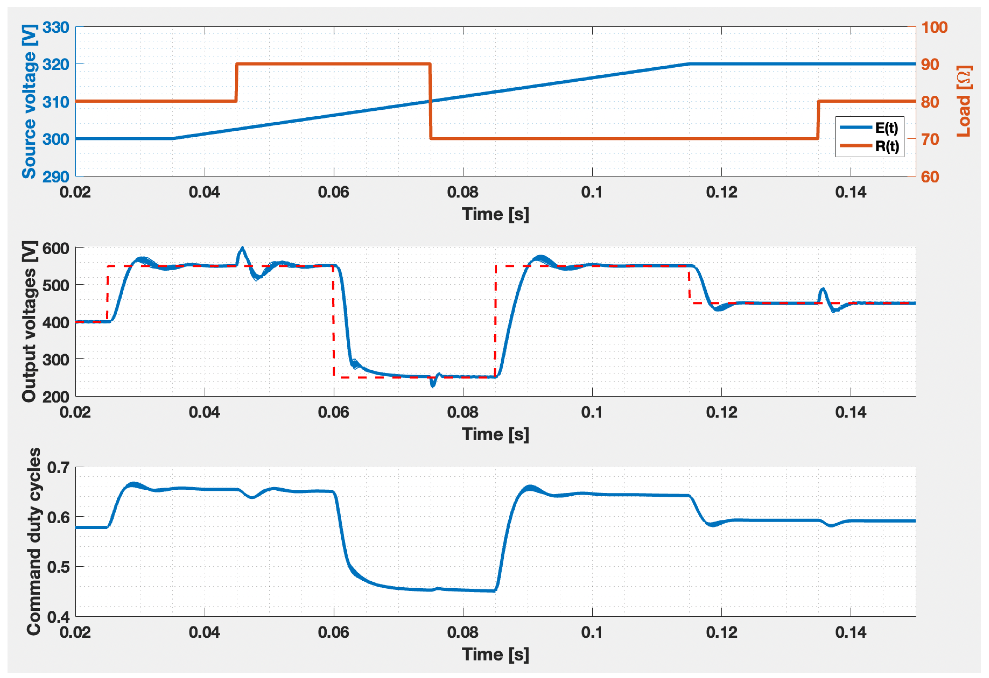
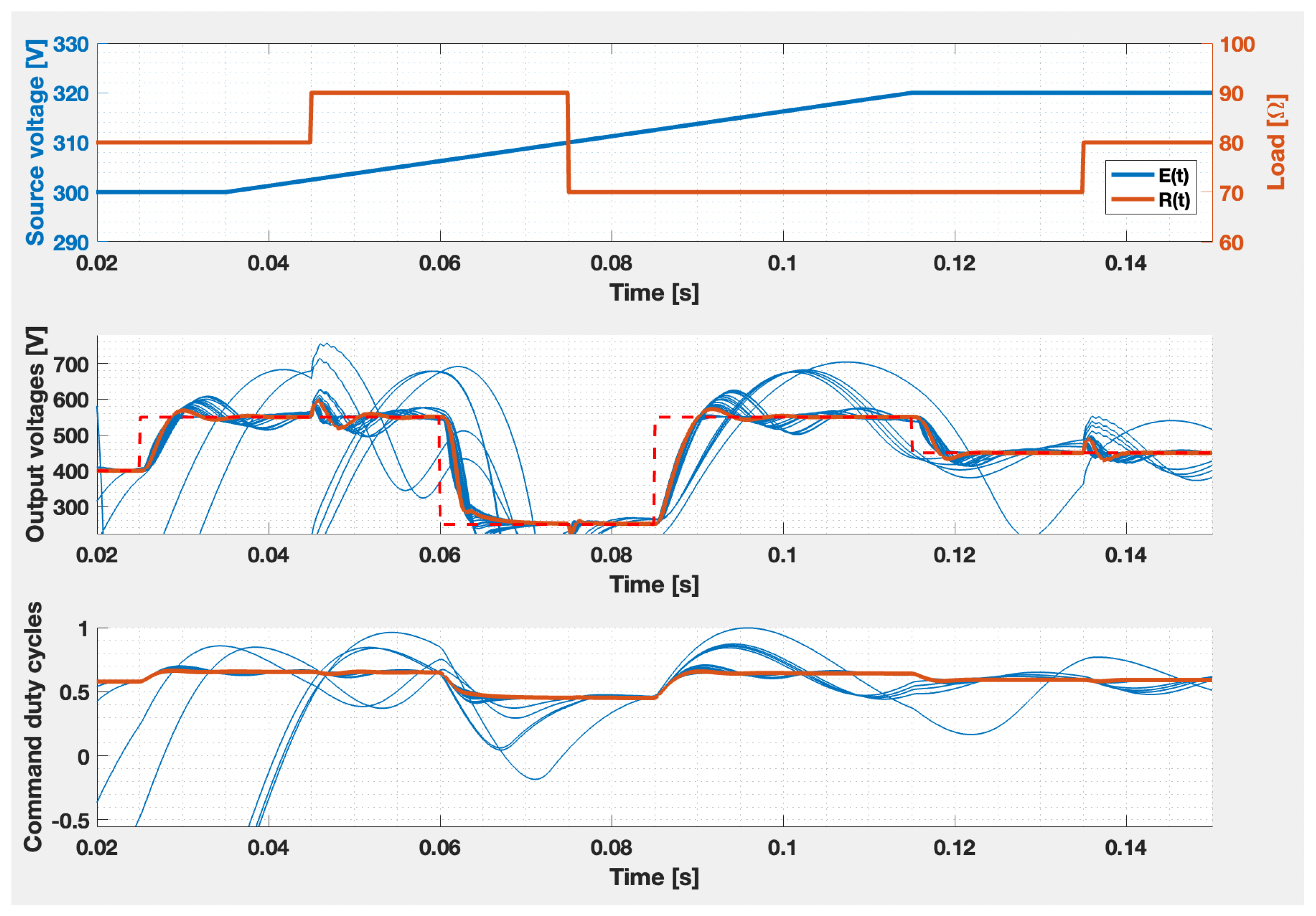
After 5 DK iterations, the resulting controller is of order 10, with an upper bound of the structural singular value equal to 0.8835 < 1 , which guarantees that the controller ensures robust stability, along with robust performance. Moreover, after an order-reduction step using the balanced model truncation method, a 3rd order controller which also maintains both RS and RP is:    
K rob SEPIC ( s ) : 1.996 3.233 4.02 0.5323 3.233 2218 6800 0.4308 4.025 6800 1.824 × 10 4 0.5359 0.5323 0.4308 0.5359 0 .
As such, the outer linear closed-loop system has the dominant poles s ^ o 1 , 2 = 67.644 ± 804.29 j , which implies that the dominant dynamics of the inner system must be at least twice as fast as Re { s o 1 } 68 . We thus consider λ ¯ = 150 as a hyperparameter of the optimization problem (31). The swarm dimension of the ABC optimization problem was N = 2000 . After e i g h t such iterations, the controller which minimizes the sensitivity of the resulting inner closed-loop system has the parameters α = 1 × 10 3 and K 2 = 8.9189 × 10 4 .
The resulting cascade control scheme has the structure proposed in Figure 1, where the plant Σ is the bilinear representation of the linearized SEPIC DC-DC converter, the inner controller K K - PBC is the proposed Krasovskii passivity-based controller, while the outer dynamical path-planning K rob was designed using the robust control framework. The difference between the desired reference value y and the measured output y is fed into the dynamical path planning, which computes the trajectory u which must be tracked by the inner loop.
The numerical results of the proposed control scheme are illustrated in Figure 4. The exogenous disturbance inputs are represented in the first row, with the additional reference signal adjacent to the output signals shown in the second row, and they vary as follows:
  • The external voltage E ( t ) has an initial value of 300 (V), while at t 1 = 0.035 (s) a ramp evolution is present until t 2 = 0.115 (s) when the value of 320 (V) is reached;
  • the output load R ( t ) has an initial value of 80 ( Ω ) , while at t 3 = 0.045 (s) its value is 90 ( Ω ) and 70 ( Ω ) at t 4 = 0.075 (s), the final value being again 80 ( Ω ) ;
  • the reference signal y has an initial value of 400 (V), and is successively changed to 550 (V) at t 5 = 0.025 (s), to 250 (V) at t 6 = 0.06 (s), to 550 (V) at t 7 = 0.085 (s), and to 450 (V) at t 9 = 0.115 (s).
The reference signal is represented with a dotted red line in the second row of the same figure, where with blue indicates the 30 Monte Carlo simulations of the closed-loop system with uncertain nonlinear plants considered. It can be noticed that the reference signal is successfully tracked with a settling time of t s 0.01 (s), and also all disturbances in terms of E and R are successfully rejected after the same duration. Moreover, the duty cycle presented in the third row of the figure manages to fulfill the constraints imposed by the physical process.

5. Discussion

In order to prove the importance of this design step, a set of numerical simulations with several configurations of parameters α and K 2 has been performed in the otherwise same conditions: the evolution of the exogenous inputs E, R and the reference signal y remain the same, as noticeable in Figure 5. Starting from the sub-optimal values of the K-PBC parameters α and K 2 , 30 Monte Carlo simulations have been performed considering values for α and K 2 in a two-decade range centered in the sub-optimal value of each parameter, while for the process, only the nominal case has been considered, for brevity. It can be noticed that the closed-loop system having the K-PBC parameters obtained as a solution of the proposed optimization problem presents a good tracking regime and good disturbance rejection, while other configurations of the parameters lead to practically unfeasible responses, with high overshoot and settling time. Moreover, the duty cycle cannot be maintained between the values of 0 and 1 as physically required, and the saturation applied for the command signal leads to even worse time-domain performance. As such, the optimization step is mandatory in order to obtain parameters for the Krasovskii passivity-based controller which lead to desirable time performance and reduce the sensitivity to the uncertainties presented in the process.
Moreover, in a similar manner to the ad hoc approach presented in our previous paper [19], the evolution of the dominant eigenvalues of the Jacobian of the LLFT connection between the plant Σ and the K-PBC is shown in Figure 6 considering values for α { α / 100 , α / 10 , α , α · 10 , α · 100 } and for K 2 { K 2 / 100 , K 2 / 10 , K 2 , K 2 · 10 , K 2 · 100 } . As noticed, there are combinations which can lead to a smaller sensitivity of these dominant eigenvalues but having a position close to the stability limit, which leads to worse performance indices, as noticed in Figure 5. As such, the proposed Problem 1 can be used if only the stabilization problem is relevant without any additional interest in terms of proposed performance, while a solution of Problem 2 manages to additionally fulfill a desired set of performance indices, especially via the dynamical path-planning component. The time-domain simulations from Figure 4 and Figure 5 were performed using the following settings: the variable-order method for fully implicit equations ode15i from MATLAB, with a relative tolerance of 10 6 and by controlling the step error using the norm of the solution, compared to its absolute value alternative. This solver was considered due to its numerical robustness for more complicated control system architectures, as utilized in Figure 1.
In order to better illustrate the differences between the ad hoc analysis presented in our previous conference paper [19] and the results presented in the previous sections, the evolution of the cost functional f u ¯ , ε ( α , k 2 ) from (30) is illustrated in Figure 7. The left subfigure presents the evolution of the functional over the entire grid, while the right side subfigure displays only the feasible zone, i.e., only where the resulting closed-loop system has the dominant dynamics under the prescribed threshold. Additionally, both plots also have the following elements: the sub-optimal values of the K-PBC’s parameters are marked with a red circle, while the optimal value of the parameters determined with the ad hoc analysis is marked with the purple circle; also, the dotted red line represents the points considered for choosing the value of α by keeping K 2 constant, which is followed by a second iteration represented with a continuous red line where the value of parameter α has been fixed and the value of parameter K 2 was selected. It can be noticed that the ad hoc analysis considers only two straight line trajectories (one horizontal direction and one vertical direction) resulting in a point which is near the feasible zone without ensuring the minimum sensitivity of the resulting inner closed-loop system, while the optimization-based technique presented in this paper is able to find the nearly-optimal value of the controller parameters by searching only in the feasible region and exploring all possible directions.

6. Conclusions

The current paper manages to present an optimization-based technique to find the sub-optimal values of the PI-type Krasovskii passivity-based controller parameters which can successfully replace the initially-proposed ad hoc analysis from our previous paper [19]. The sensitivity analysis of the Krasovskii passivity-based controller has been studied by introducing a functional which describes the length of the curve of the dominant eigenvalue of the Jacobian of the resulting inner closed-loop system. However, the resulting optimization problem is non-convex by nature, which leads to the necessity of using a global metaheuristic approach in order to find a sub-optimal set of parameters. As such, for the purpose of this paper, we considered a modified version of the artificial bee colony optimization technique. The main modifications are in terms of stopping criteria, all modifications leading to an increased execution speed of the algorithm by avoiding the search in the unfeasible domain. Moreover, the benefit of the proposed method has been illustrated on a nonideal DC-DC SEPIC converter. The Numerical Results section presents an end-to-end approach to design both the Krasovskii passivity-based controller and dynamic path planning for the proposed process modeled as a bilinear system.
As further research directions, the following ideas are of interest: (i) formulating the optimization problem for a more general class of nonlinear systems, starting from the idea presented in [14]; (ii) formulating a similar optimization problem in a convex manner in terms of linear matrix inequalities; (iii) directly including the matrix Q in the optimization problem with greater possibilities of ensuring a better set of performances, but with the downside of increasing the dimensionality of the problem; (iv) studying the quantization effects of the proposed method for the practical implementability of the proposed structure.

Author Contributions

Conceptualization, V.M.; methodology, V.M.; software, V.M. and M.Ş.; validation, M.Ş., D.M. and P.D.; formal analysis, V.M. and P.D.; investigation, V.M.; resources, V.M.; data curation, M.Ş. and D.M.; writing—original draft preparation, V.M.; writing—review and editing, M.Ş. and D.M.; visualization, P.D.; supervision, P.D.; project administration, V.M.; funding acquisition, P.D. All authors have read and agreed to the published version of the manuscript.

Funding

This paper was financially supported by the Project “Entrepreneurial competences and excellence research in doctoral and postdoctoral programs—ANTREDOC”, project co-funded by the European Social Fund financing agreement no. 56437/24.07.2019.

Data Availability Statement

Not applicable.

Conflicts of Interest

The authors declare no conflict of interest.

Abbreviations

The following abbreviations are used in this manuscript:
ABCArtificial Bee Colony
DCDirect Current
K-PBCKrasovskii Passivity-Based Controller
LFTLinear Fractional Transform
LLFTLower Linear Fractional Transform
LMILinear Matrix Inequality
LTILinear and Time-Invariant
NPNon-Deterministic Polynomial Time
PBCPassivity-Based Controller
PIProportional–Integrative
RCFRobust Control Framework
SISOSingle-Input Single-Output
SEPICSingle-Ended Primary-Inductor Converter
S-PBCShifted Passivity-Based Controller
ULFTUpper Linear Fractional Transform

References

  1. Willems, J.C. Dissipative dynamical systems part II: Linear systems with quadratic supply rates. Arch. Ration. Mech. Anal. 1972, 45, 352–393. [Google Scholar] [CrossRef]
  2. Khalil, H. Nonlinear Systems; Prentice Hall: Prentice, NJ, USA, 1996. [Google Scholar]
  3. van der Schaft, A.J. L2-Gain and Passivity Techniques in Nonlinear Control, 3rd ed.; Springer: Cham, Switzerland, 2017. [Google Scholar]
  4. Bao, J.; Lee, P.L. Process Control—The Passive Systems Approach, 1st ed.; Springer: London, UK, 2007. [Google Scholar]
  5. Pavlov, A.; Marconi, L. Incremental passivity and output regulation. In Proceedings of the 45th IEEE Conference on Decision and Control, San Diego, CA, USA, 13–15 December 2006. [Google Scholar]
  6. Pang, H.; Zhao, J. Incremental passivity and output regulation for switched nonlinear systems. Int. J. Control 2017, 90, 2072–2084. [Google Scholar] [CrossRef]
  7. van der Schaft, A.J. On differential passivity. IFAC Proc. Vol. 2013, 46, 21–25. [Google Scholar] [CrossRef] [Green Version]
  8. Forni, F.; Sepulchre, R.; van der Schaft, A.J. On differential passivity of physical systems. In Proceedings of the 52nd IEEE Conference on Decision and Control, Firenze, Italy, 10–13 December 2013; pp. 6580–6585. [Google Scholar]
  9. Li, N.; Scherpen, J.; van der Schaft, A.; Sun, Z. A passivity approach in port-Hamiltonian form for formation control and velocity tracking. In Proceedings of the 2022 European Control Conference (ECC), London, UK, 12–15 July 2022. [Google Scholar]
  10. Simpson-Porco, J.W. Equilibrium-Independent Dissipativity With Quadratic Supply Rates. IEEE Trans. Autom. Control 2019, 64, 1440–1455. [Google Scholar] [CrossRef] [Green Version]
  11. Kosaraju, K.C.; Kawano, Y.; Scherpen, J.M.A. Krasovskii’s Passivity. In Proceedings of the 11th IFAC Symposium on Nonlinear Control Systems NOLCOS, Vienna, Austria, 4–6 September 2019; Volume 52, pp. 466–471. [Google Scholar]
  12. Kawano, Y.; Kosaraju, K.C.; Scherpen, J.M.A. Krasovskii and Shifted Passivity-Based Control. IEEE Trans. Autom. Control 2021, 66, 4926–4932. [Google Scholar] [CrossRef]
  13. Mihaly, V.; Şuşcă, M.; Dobra, P. Krasovskii Passivity and μ-Synthesis Controller Design for Quasi-Linear Affine Systems. Energies 2021, 14, 5571. [Google Scholar] [CrossRef]
  14. Mihaly, V.; Şuşcă, M.; Morar, D.; Dobra, P. Polytopic Robust Passivity Cascade Controller Design for Nonlinear Systems. In Proceedings of the 22nd European Control Conference, London, UK, 13–15 July 2022. [Google Scholar]
  15. Silani, A.; Cucuzzella, M.; Scherpen, J.M.A.; Yazdanpanah, M.J. Robust output regulation for voltage control in DC networks with time-varying loads. Automatica 2022, 135, 109997. [Google Scholar] [CrossRef]
  16. Geromel, J.C.; Colaneri, P.; Bolzern, P. Passivity of switched linear systems: Analysis and control design. Syst. Control Lett. 2012, 61, 549–554. [Google Scholar] [CrossRef]
  17. Hughes, T.H. A theory of passive linear systems with no assumptions. Automatica 2017, 86, 87–97. [Google Scholar] [CrossRef] [Green Version]
  18. Hughes, T.H. On reciprocal systems and controllability. Automatica 2019, 101, 396–408. [Google Scholar] [CrossRef]
  19. Mihaly, V.; Şuşcă, M.; Morar, D.; Dobra, P. Closed-Loop System Sensitivity Analysis for Passivity-Based Controller Parameters. In Proceedings of the IEEE International Conference on Automation, Quality and Testing, Robotics, Cluj-Napoca, Romania, 19–21 May 2022. [Google Scholar]
  20. Pham, D.T.; Ghanbarzadeh, A.; Koc, E.; Otri, S.; Rahim, S.; Zaidi, M. The Bees Algorithm; Technical Note; Manufacturing Engineering Centre, Cardiff University: Cardiff, UK, 2005. [Google Scholar]
  21. Şuşcă, M.; Mihaly, V.; Stănese, M.; Morar, D.; Dobra, P. Unified CACSD Toolbox for Hybrid Simulation and Robust Controller Synthesis with Applications in DC-to-DC Power Converter Control. Mathematics 2021, 9, 731. [Google Scholar] [CrossRef]
  22. Packard, A.; Doyle, J.; Balas, G. Linear Multivariable Robust Control with a μ Perspective. J. Dyn. Syst. Meas. Control 1993, 115, 426–438. [Google Scholar] [CrossRef]
  23. Balas, G.; Chiang, R.; Packard, A.; Safonov, M. Robust Control Toolbox—User’s Guide; The MathWorks: Natick, MA, USA, 2020. [Google Scholar]
Figure 1. The resulting closed-loop system composed of an inner loop which consists of an LLFT interconnection between the plant Σ and K-PBC, ensuring the passivity of the closed-loop inner system, along with an outer loop containing a dynamic path planning represented by the robust controller K rob designed to ensure robust performance.
Mathematics 10 03750 g001
Figure 2. Path-planning regulator design methodology using the closed-loop shaping robust control framework, which can impose the desired bandwidth compared to the K-PBC from Figure 1 [21].
Mathematics 10 03750 g002
Figure 3. Electrical schemes of nonideal SEPIC DC-DC converter.
Mathematics 10 03750 g003
Figure 4. The averaged bilinear model of the DC-DC SEPIC converter for both nominal plants, along with 30 Monte Carlo simulations according to Figure 1 and using the sub-optimal parameters α = 1 × 10 3 and K 2 = 8.9189 × 10 4 of the K-PBC; the first plot—the exogenous inputs, the second plot—the reference signal (dotted red) and the output voltage (blue), and the third plot—the command signal.
Mathematics 10 03750 g004
Figure 5. Average nominal bilinear DC-DC SEPIC converter model with 30 parameters sets for the K-PBC around sub-optimal values α = 1 × 10 3 , K 2 = 8.9189 × 10 4 ; the first plot—exogenous inputs, the second plot—reference (dotted red) and output voltage: sub-optimal (orange) versus other configurations (blue); the third plot—command signal: sub-optimal case (orange) and other configurations (blue).
Mathematics 10 03750 g005
Figure 6. The evolution of the dominant eigenvalues of the Jacobian of the inner closed-loop system considering 100 experimental forced-equilibrium points which correspond to an input signal from the closed ball B ( u ¯ = 0.5 , ε = 0.1 ) for the sub-optimal values α = 1 × 10 3 and K 2 = 8.9189 × 10 4 , along with 24 other experiments where these parameters vary by two decades on the left and right sides.
Mathematics 10 03750 g006
Figure 7. The evolution of the cost function f u ¯ , ε in terms of α and k 2 with (right) and without (left) considering the feasible region, along with the location of the sub-optimal solution (red circle), the location of the solution obtained based in the ad hoc analysis (purple circle), and the two iterations used in the ad hoc analysis (dotted red and red lines).
Mathematics 10 03750 g007
Table 1. Nominal circuit element values and tolerances for the SEPIC DC-DC converter.
ParameterNominal ValueToleranceParameterNominal ValueTolerance
L 1 2.57 (mH) ± 20 % L 2 1.71 (mH) ± 20 %
r L 1 130 (m Ω ) ± 10 % r L 2 110 (m Ω ] ± 10 %
r D S 1 0.01 ( Ω ) ± 10 % r D S 2 80 (m Ω ) ± 10 %
C 1 4.7 ( μ F) ± 20 % C 2 3.57 ( μ F) ± 20 %
r C 1 270 (m Ω ) ± 10 % r C 2 350 (m Ω ) ± 10 %
C i n 3.57 ( μ F) ± 20 % r C i n 270 (m Ω ) ± 10 %
V F 1 0.2 (V) ± 10 % V F 2 0.62 (V) ± 10 %
Publisher’s Note: MDPI stays neutral with regard to jurisdictional claims in published maps and institutional affiliations.

