Abstract
The extreme value theory is widely used in economic and environmental domains, it aims to study the stochastic extreme behaviors associated with rare events. In this context, we consider a new mixture model for extremal events analysis, including a Dirichlet process mixture of Weibull (DPMW) distribution below the threshold and the point process (PP) extreme model for the upper tail. This model developed a regression structure for the PP extreme model parameters, which explains the variation of the exceedance through all tail parameters. The estimation of the model parameters is performed under the Bayesian paradigm, applying the Markov chains Monte Carlo (MCMC) method. The model is applied to both simulation and real environmental data to demonstrate the performance in extrapolating extreme events.
Keywords:
extreme value; mixture model; Dirichlet process mixture; regression structure; Bayesian inference MSC:
62F15; 62G32
1. Introduction
Extreme value models have been widely studied to analyze extreme events of maximum and minimum in environmental sciences, engineering and financial econometrics. Coles [1] showed that the motivation of extreme value models is to prevent extreme event damages, because, even though their probability of occurrence is small, their consequences can be undesirable.
The Generalized Pareto Distribution (GPD) describes a limit distribution of exceedance above the threshold, it consists of modeling the tail of the data. The GPD denoted by with threshold u, scale parameter and shape parameters . Coles and Tawn [2] and Coles [1] showed that the parameter is strongly dependent on the threshold u in the GPD model, i.e., , where and are the scale parameter and location parameter of the Generalized Extreme Value (GEV) model, respectively. The dependence between the parameters can lead to poor mixing [3]. Pickands [4,5] consider a more general tail model, point process (PP) extreme model, which can more easily be extended to the non-stationary case by allowing a change in the number of threshold exceedances over time.
The more common approaches for the PP models are to fix the threshold u where it is necessary to give a lot of attention in choosing this threshold, the different choices of u often result in very different parameter estimates and inferences [1,6]. Therefore, an extreme value mixture model is presented to avoid the selection threshold, which is the distribution below the threshold and an extreme value model in the tail. Frigessi et al. [7] suggested to model the data with a dynamical mixture, one component is a GPD and a lighter Weibull distribution as the other component, using maximum likelihood to estimate the approximate standard deviations. Behrens et al. [8] introduced a mixture model which combines a gamma distribution for the center and a GPD for the tail, using all observations for inference about the unknown parameters from both distributions, the threshold included. MacDonald et al. [3] proposed an extreme value mixture model where one term of the mixture is the non-parametric kernel density distribution, and the other is the point process model. However, all the prior of the parametric model in the bulk part of the aforementioned approach is specific, it follows that the parameter density estimation is complicated.
In this paper, we present a new flexible point process regression extreme model using a Dirichlet process mixture of Weibull distribution (DPMW-PPR), the presented model can be used to control the number of components by the Dirichlet process mixture model without prior information. Athanasios Kottas [9] showed that Dirichlet process (DP) mixture models form a very rich class of Bayesian nonparametric models. DP mixture models emerge by employing a DP prior for the mixing distribution in a mixture of a parametric family of distributions [10,11]. Hanson [12] and Jairo [13] proposed the DP mixture of gamma densities in the bulk part below the threshold and estimated the univariate densities on the positive real line. Here, we introduce the new point process regression extreme model includes a Dirichlet process mixture Weibull (DPMW) distribution below the threshold and the point process (PP) extreme model above the threshold. Moreover, the model established the addition of a regression structure for the estimation of the PP model parameters, based on the Bayesian approach, the prior distributions will not be attributed directly to the parameters of the PP extreme model, but to the coefficients of their linear structure. There are three key ingredients in our approach: we model all data, not only those belonging to the tail; we use a mixture model, one component of which is a Dirichlet process mixture of Weibull (DPMW) distribution and the other component with a point process (PP) extreme model; and we develop a regression structure for the PP model parameters, which explains the variation of the exceedance through all tail parameters. With the DPMW distribution under the threshold, the proposed model works well even in the absence of prior distribution and small sample sizes. The regression structure for the PP model parameters explains the behavior of the time series.
This work is divided into the following parts. In Section 2, we present the new mixture extreme model. In Section 3, we provide the MCMC method to make Bayesian inference for the model parameters. The simulation study of the proposed model with different sample sizes is provided in Section 4. In Section 5, two real environmental data are fitted to the proposed model. Finally, Section 6 shows the concluding remarks.
2. A New Point Process Regression Extreme Model
The proposed model assumes that observations below the threshold u follow a distribution with parameters , here with , while the observations above the threshold are from a point process (PP) extreme model.
Pickands [4] showed that the point process defined by
is well approximated, in the limit as , by an inhomogeneous Poisson process on the region , for a sufficiently high threshold u, with the intensity function on the subregion given by
where , the scaling constant is the number of blocks of observations (e.g., number of years of daily data) and is the parameter of PP extreme model.
Therefore, the distribution function F, of a sequence of n identically and independent distributed observations can be written as
where is the PP extreme model defined by (1). The density of the model is shown as:
where denotes the density of and denotes the density of PP.
2.1. The DPMW Densities
This paper uses the Dirichlet process mixture of Weibull (DPMW) distribution in the bulk part of Equation (2). The DP consists of a parametric distribution function , the center or base distribution of the process, and a positive scalar precision parameter v [9]. The is shown as a DP prior of the distribution function H. Then, we obtain the DP mixture model
where is the distribution function of the parametric kernel of the mixture and . If is the density corresponding to , the density of the random mixture in (4) is .
The Dirichlet process mixture of Weibull distribution has been considered by Kottas [9] for the survival data. The Weibull distribution with the shape parameter a and scale parameter b is given by
where and .
Similar to [9], we use a non-conjugate uniform inverse gamma probability density distribution for the unknown parameters,
here, denotes the inverse gamma distribution with mean , provided .
Since the Pareto distribution is conjugated to the uniform distribution, we use it as the prior for .
by default , which is an infinite variance prior distribution.
The conjugate prior of b is the gamma distribution since it comes from the inverse gamma distribution with the fixed shape .
We set , , and by default.
The full Bayesian model can be written in the following hierarchical form:
with defined in (6), d and all parameters of the priors of v, and are fixed.
2.2. Regression Structure for PP Parameters
The likelihood function of the extreme mixed model in (2) can be separated into the bulk distribution model and the PP tail model, as shown here:
we define as the parameter vector.
The likelihood function of the PP model is given by:
where , and is the number of exceedances of the threshold u, see [14,15].
The model developed has the addition of a regression structure for the estimation of the PP parameters, in which the prior distributions will not be attributed directly to the parameters, but to the coefficients of their linear structure [16,17]. Let parameters u, , , have the dimensional covariate vector: , with the first component of each of these vectors being equal to 1 allowing the inclusion of the intercept in the regression structures of the model. We will have a matrix of regression coefficients composed of the vectors , , and , with , , and , where each row of this matrix is associated with each of the parameters u, , , .
For each parameter, we will have a function that links it to its respective linear structure. In this model, we opted for a transformation in the linking function of the parameters and , which will have the following scheme:
By choosing this reparametrization, the components are orthogonal, see [18,19], which will facilitate the calculation of joint prior densities .
Thus, we have the parameters , , , estimated by the following structure:
where , , , are the estimates of the regression coefficients, are the covariate vectors of the parameters , , and , which may or may not have covariates in common.
3. Bayesian Inference
The priors for the regression coefficients of the threshold u, the scale parameter , the shape parameter and the location parameter will be presented in this section. In this work, we adopt the normal prior of the , , and , which are
Then, we have
The posterior distribution of the proposed point process regression extreme model using a Dirichlet process mixture of Weibull distribution (DPMW-PPR) is then as follows:
for and
for with and .
4. Simulation Study
The simulated mixture distribution for the central part using data generated from a mixture of lognormal distribution:
Similar as [9], we set the DP precision , and the hyperparamenters for and are , , , .
For the simulation data of the PP part, we consider the fixed threshold as the 10% of the distribution in the upper tail means that the regression coefficients and are both equal to zero and the . Following Lima [20], the first covariate vectors of the parameters is given by , representing the seasonal effect, and the second covariate is given by . We consider the regression coefficients parameters as follows
The prior of the threshold u, equal to in this simulation, is given by , where is the 90% quantile of the simulated data and is the of probability in the range between and of the simulation data.
For the regression coefficients parameters of , and , we consider the following non-informative prior distribution:
As with the usual Metropolis algorithm, we adjust the variance of the sampling proposal density by using Markov chain Monte Carlo (MCMC) simulations to consider the Hessen value of the maximum likelihood estimate. After 5000 run-in cycles, we obtained convergence for all parameters using 10,000 iterations.
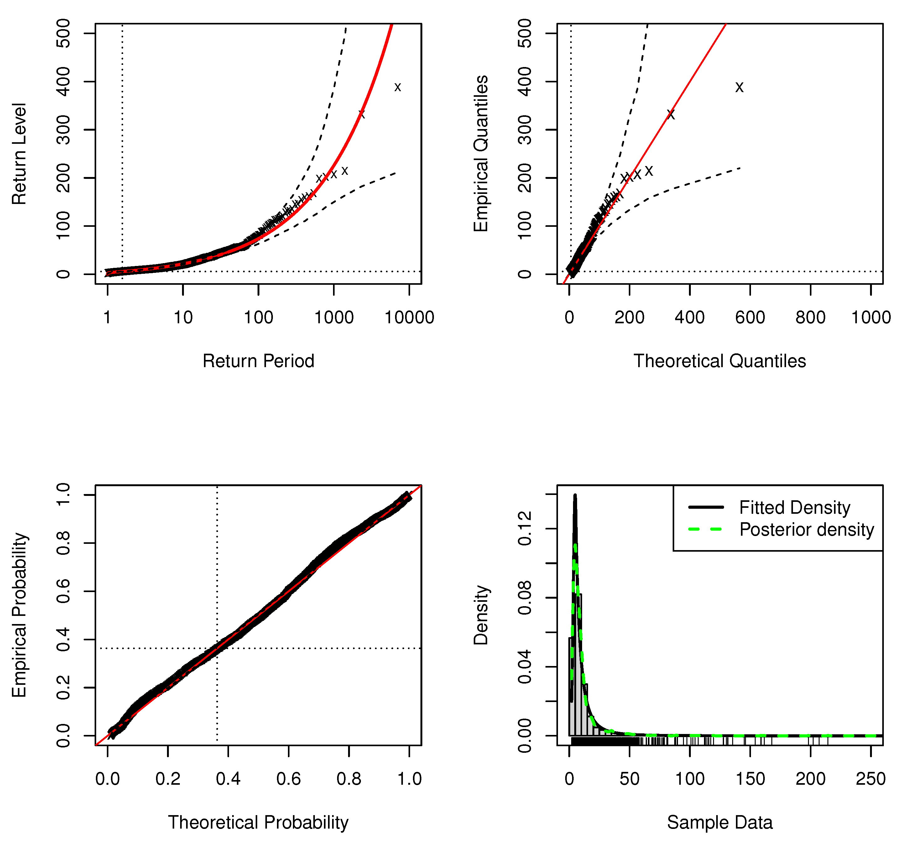
Table 1 shows the estimates for the regression coefficients of simulations with sample , and the estimate of threshold u is with the credibility interval . The standard model fit diagnostics for the upper tail of the DPMW-PPR model is plotted in Figure 1, which indicates no issues with the upper tail fit. The standard model fit diagnostics for the full range values of the DPMW-PPR model is plotted in Figure 2, indicating an adequate fit over the observed range of support.

Table 1.
Estimates for the regression coefficients of simulations with sample .
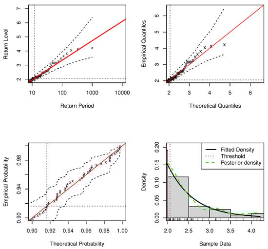
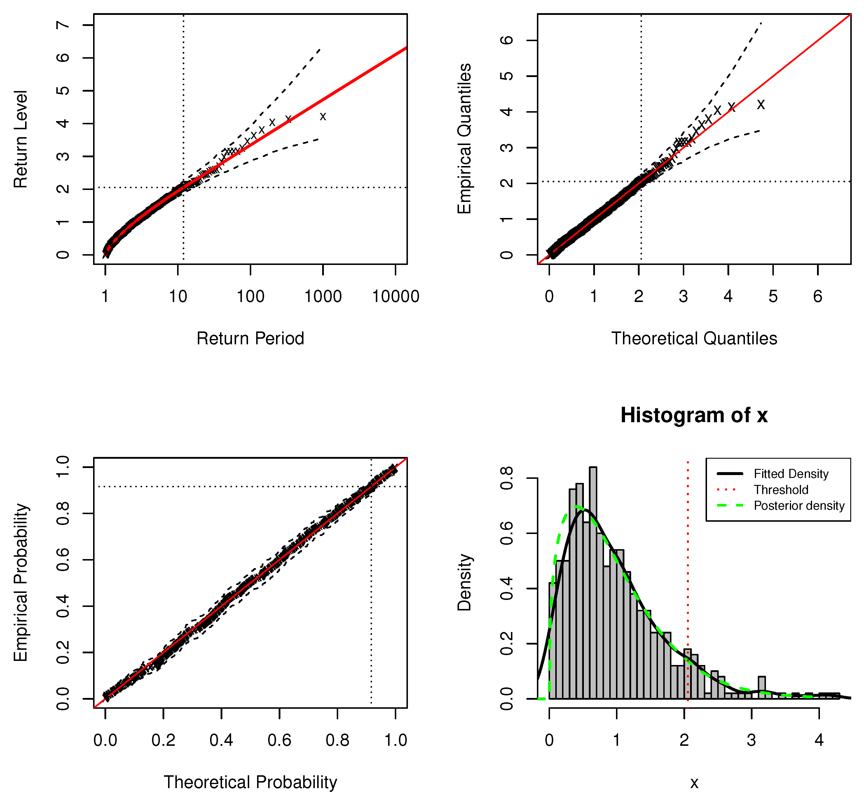
Figure 1.
Standard model fit diagnostics for the upper tail of the DPMW-PPR model fitted to the simulated data with . (The top left corner is the return level plot, the top right corner is the quantile plot, the bottom left corner is the probability plot, and the bottom right corner is the density plot).
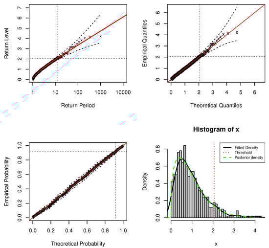
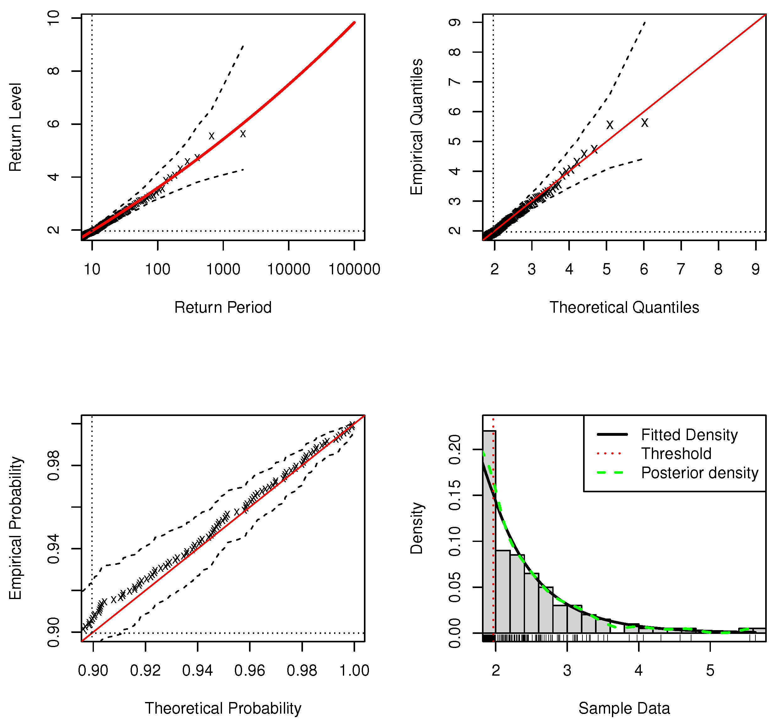
Figure 2.
Standard model fit diagnostics for the DPMW-PPR model fitted to the simulated data with . (The top left corner is the return level plot, the top right corner is the quantile plot, the bottom left corner is the probability plot, and the bottom right corner is the density plot).
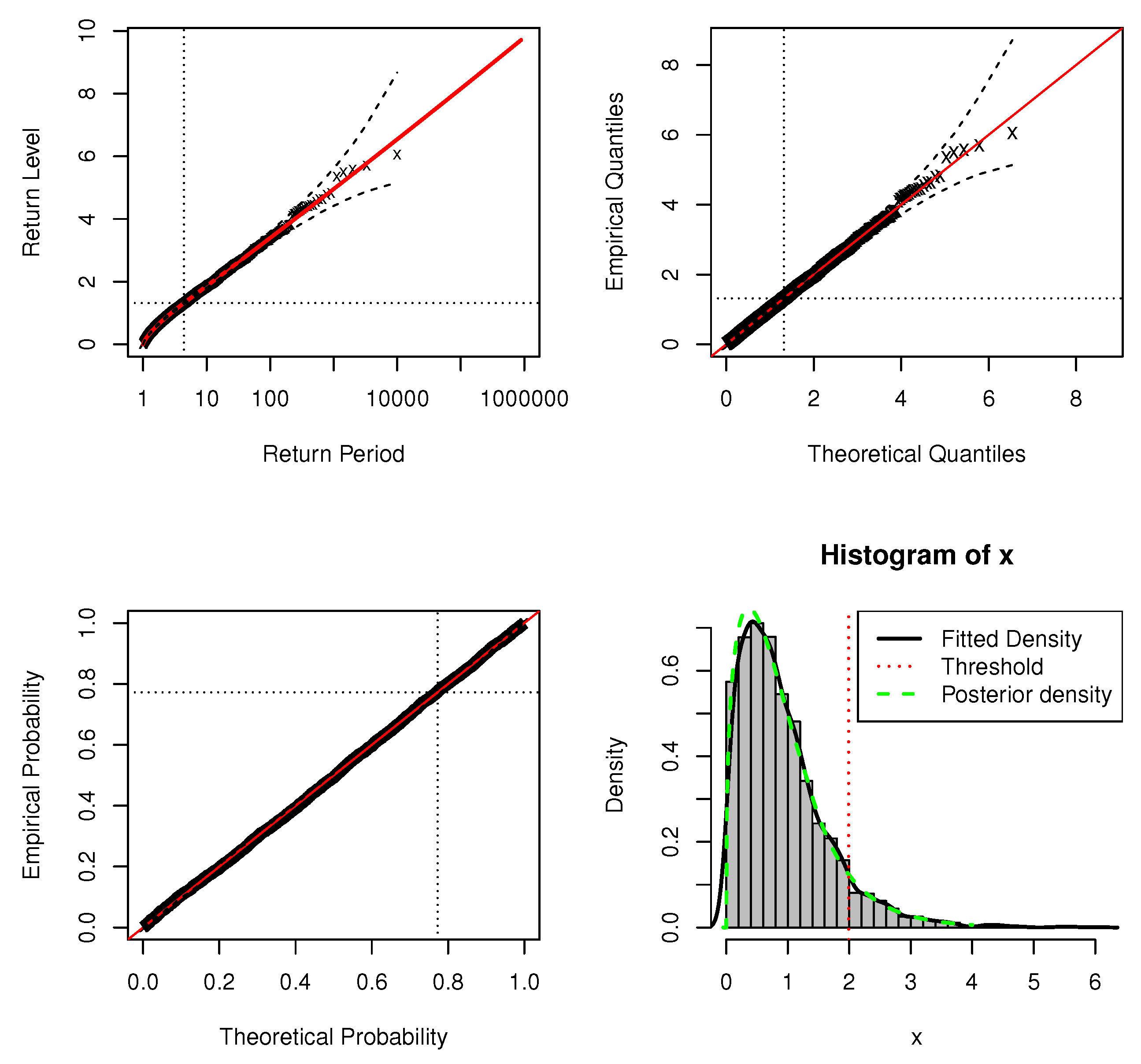
In standard model fit diagnostics figures, the top left corner is the return level plot, the top right corner is the quantile plot, the bottom left corner is the probability plot, and the bottom right corner is the density plot. In the return level plot, the points are the simulation data, the red line is the return level line fitted to the DPMW-PPR model, the dashed lines illustrate the credibility interval of the return level, and the two dotted lines are the upper tail fraction and threshold. In the quantile plot, the points are the simulation data, the line of equality is illustrated as the red line, the dashed lines illustrate the credibility interval, and the dotted lines are the thresholds. In the probability plot, the points are the simulation data, the line of equality is illustrated as the red line, the dashed lines illustrate the credibility interval, and the dotted lines are the upper tail fractions. In the density plot, the black solid line shows the true density function, the green dashed line shows the posterior predictive density function, and the red dashed line shows the estimate of threshold u.
In Figure 1 and Figure 2, we can see that both the probability and quantile plots show the effectiveness of the fitted model: each set of points plotted is nearly linear. The return level curves are close to linear, they also provide a satisfactory representation of the empirical estimates, especially once sampling variability is taken into account. The density plots in the bottom right corners of both figures show the density histogram of 500 simulations with the true density function (black solid line), the posterior density function with regression (blue dashed line) and the red dashed line is the estimate of threshold u.
Table 2 shows the estimates for the regression coefficients of simulations with sample , and the estimate of threshold u is with the credibility interval . Table 3 shows the estimates for the regression coefficients of simulations with sample , and the estimate of threshold u is with the credibility interval . We can see some similarities compared with the previous table. In this case, as the sample size is larger, it means that we have more information about the data with respect to the parameters, and in both types of prior the length of the credibility interval is lower than their equivalent cases compared with the small sample sizes. The results show that the proposed model could be even better when large sample sizes are considered.
Table 2.
Estimates for the regression coefficients of simulations with sample .
Table 3.
Estimates for the regression coefficients of simulations with sample .
Figure 3 and Figure 4 are the standard model fit diagnostics for the upper tail and the standard model fit diagnostics for full range values of the DPMW-PPR model with sample size , respectively. Figure 5 and Figure 6 are the standard model fit diagnostics for the upper tail and the standard model fit diagnostics for the full range values of the DPMW-PPR model with sample size . These standard diagnostic graphical imply the good fit of the DPMW-PPR model. The probability and quantile plots are better than the previous example in which the sample size is , and once confidence intervals are added to the regression horizontal curve, the quality of the fit becomes more convincing.
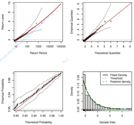
Figure 3.
Standard model fit diagnostics for the upper tail of DPMW-PPR model fitted to the simulated data with . (The top left corner is the return level plot, the top right corner is the quantile plot, the bottom left corner is the probability plot, and the bottom right corner is the density plot).
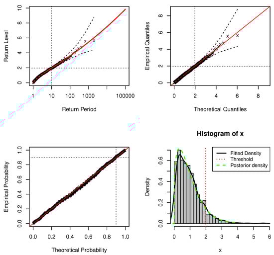
Figure 4.
Standard model fit diagnostics for the DPMW-PPR model fitted to the simulated data with . (The top left corner is the return level plot, the top right corner is the quantile plot, the bottom left corner is the probability plot, and the bottom right corner is the density plot).
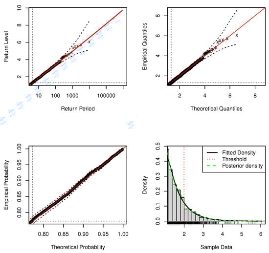
Figure 5.
Standard model fit diagnostics for the upper tail of the DPMW-PPR model fitted to the simulated data with . (The top left corner is the return level plot, the top right corner is the quantile plot, the bottom left corner is the probability plot, and the bottom right corner is the density plot).

Figure 6.
Standard model fit diagnostics for the DPMW-PPR model fitted to the simulated data with . (The top left corner is the return level plot, the top right corner is the quantile plot, the bottom left corner is the probability plot, and the bottom right corner is the density plot).
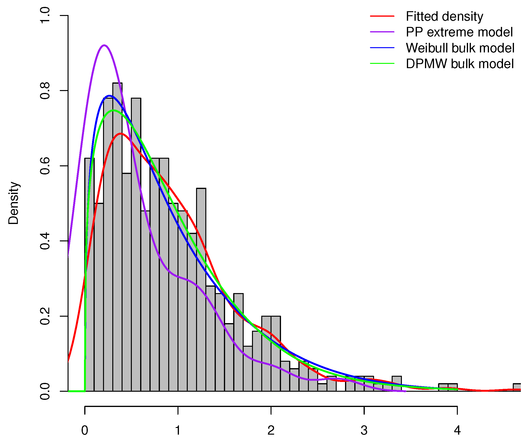
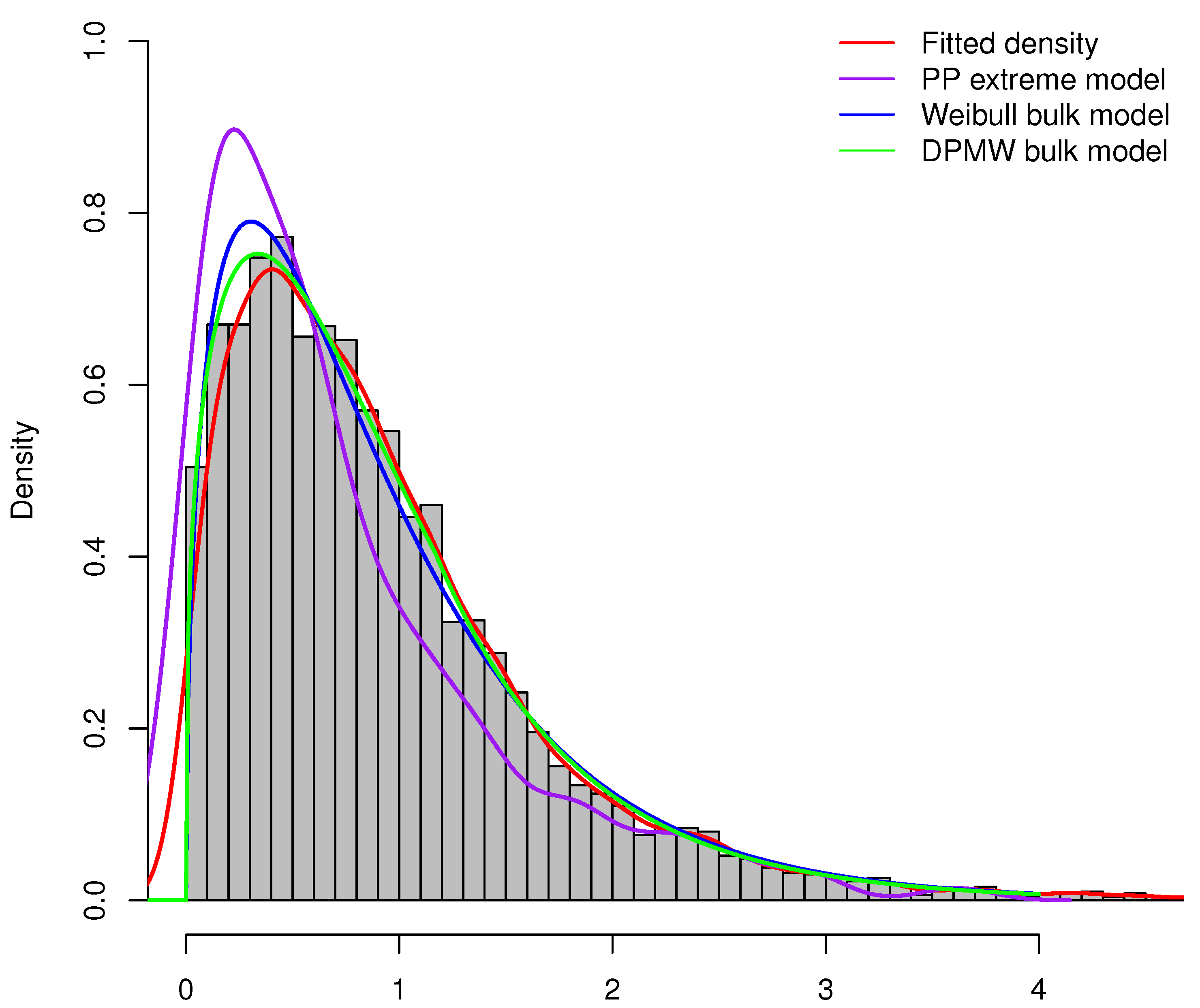
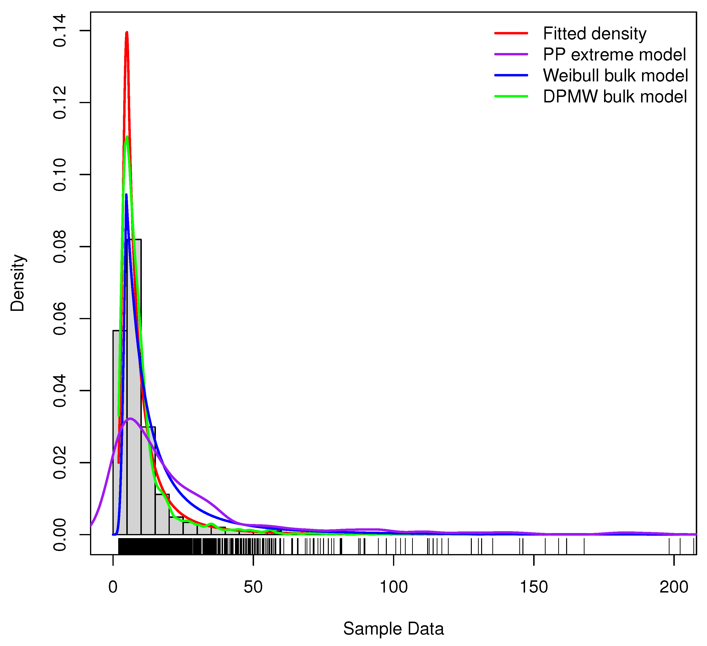
Furthermore, we compare the proposed model (DPMW-PPR) with the Point Process (PP) extreme value model and the Weibull mixture Point Process (WMPP) extreme model, which combined the Weibull distribution in the bulk part and the Point Process extreme value model in the tail [3]. Figure 7, Figure 8 and Figure 9 show the true fitted density and the posterior density of the above three models with the simulated sample size , , and , respectively. Obviously, our proposed model is superior to the other two models.
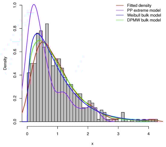
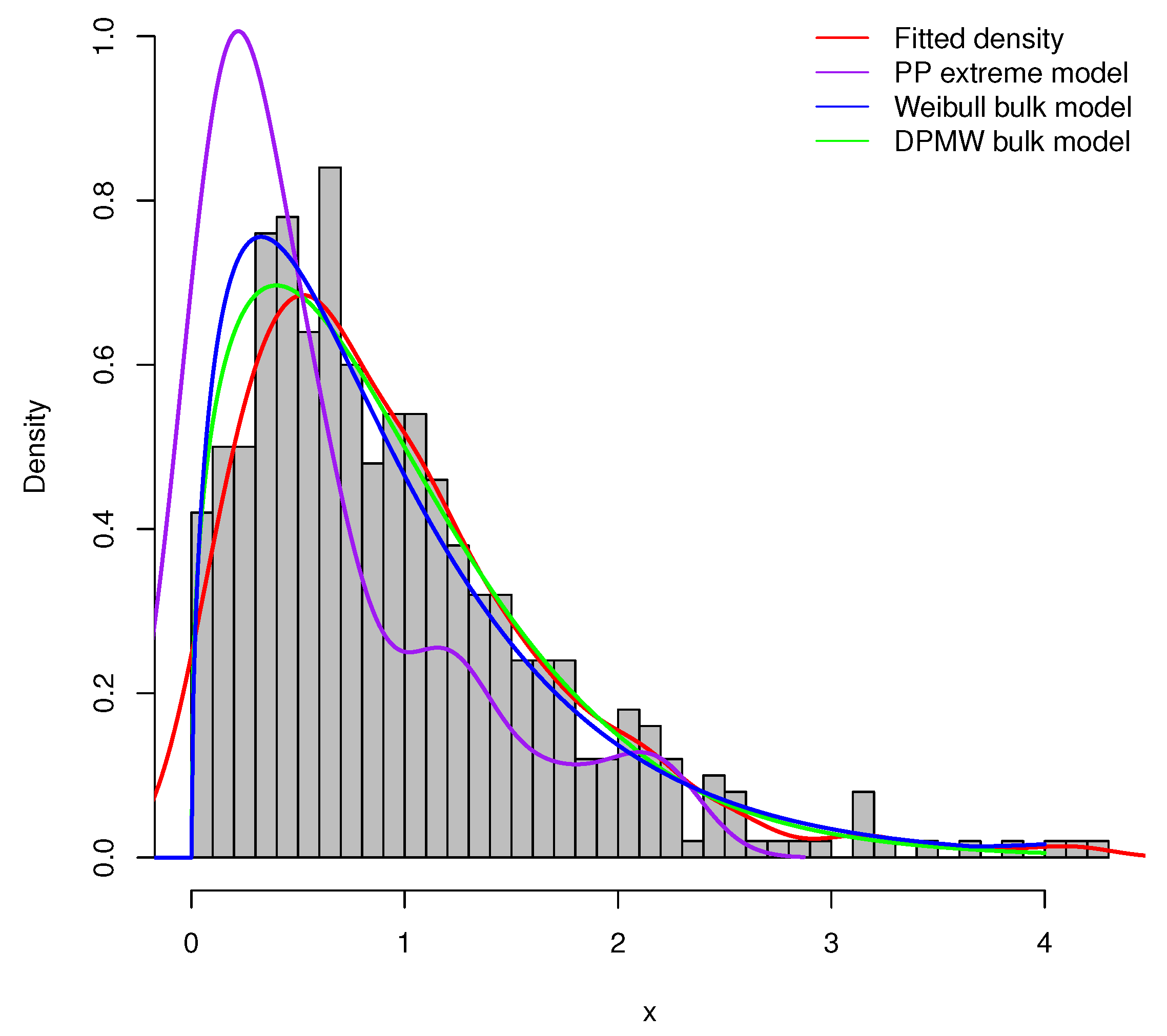
Figure 7.
The posterior density plot for three models (the DPMW-PPR model, the PP extreme value model and the WMPP extreme model) with . The red line shows the true density function, the green line, the blue line and the purple line are the posterior density function of the DPMW-PPR model, the WMPP extreme model and the PP extreme value model, respectively.
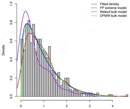
Figure 8.
The posterior density plot for three models (the DPMW-PPR model, the PP extreme value model and the WMPP extreme model) with . The red line shows the true density function, the green line, the blue line and the purple line are the posterior density function of the DPMW-PPR model, the WMPP extreme model and the PP extreme value model, respectively.
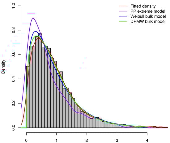
Figure 9.
The posterior density plot for three models (the DPMW-PPR model, the PP extreme value model and the WMPP extreme model) with . The red line shows the true density function, the green line, the blue line and the purple line are the posterior density function of the DPMW-PPR model, the WMPP extreme model and the PP extreme value model, respectively.
5. Application to Real Data
This section is intended for the application of the proposed model. In order to show the utility of the new model, we apply the methodology to the study of two river flow datasets (environmental data): the monthly flow data for the Iowa river measured at Wapello, IA, USA and the daily flow data for the Patuxent river observed near Bowie, MD, USA. For estimation of the model, the MCMC algorithm was run on the Windows 10 system, with a 64-bit opteron system 2.20 GHz processor with 16 GB RAM. The MCMC Metropolis-Hastings sampler was initialized at an arbitrary starting parameter vector and run for 20,000 iterations with a burn-in period of 5000, giving 15,000 posterior draws for each simulation.
5.1. The Monthly Flow in the Iowa River
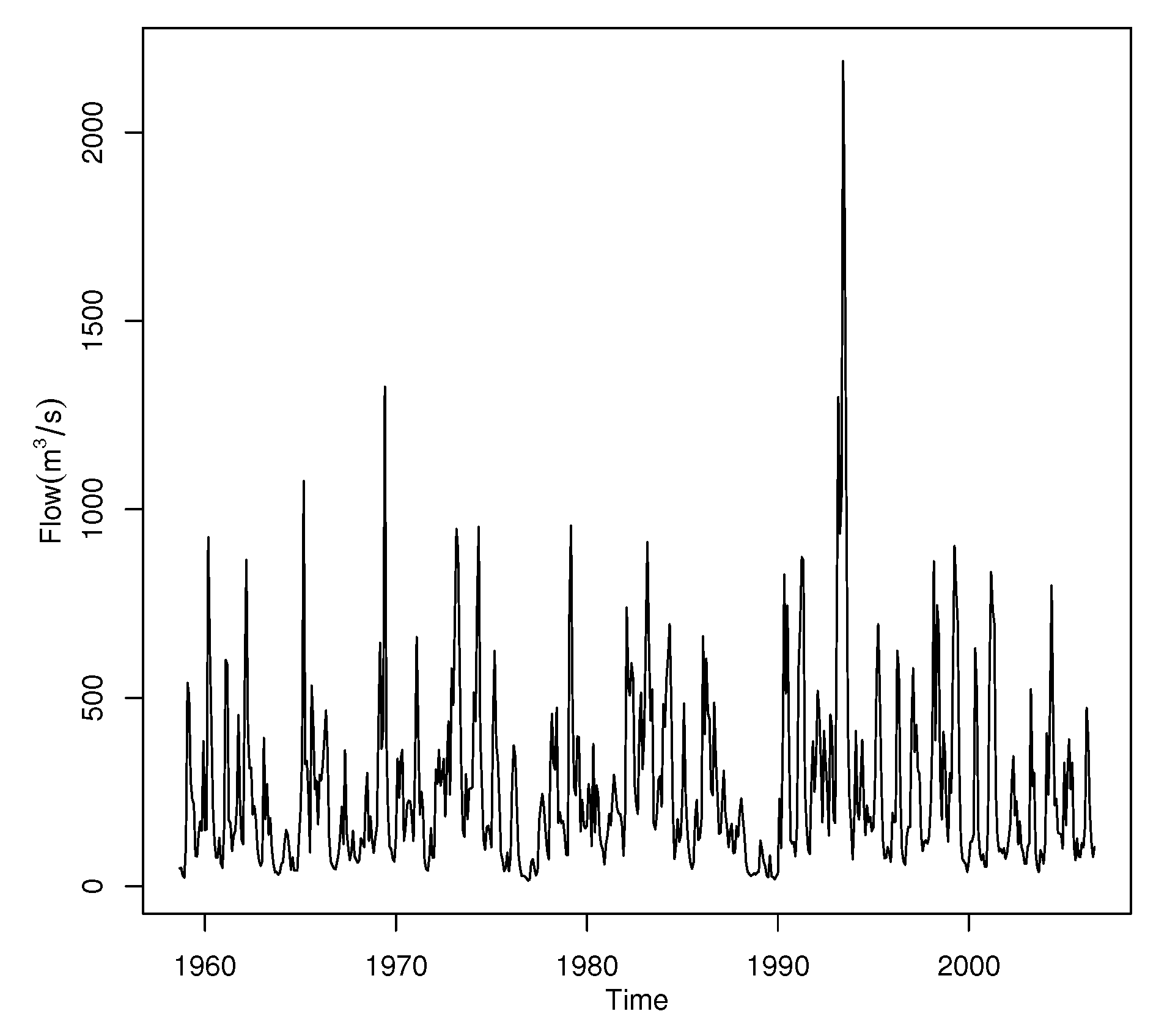
The Iowa river is a tributary of the Mississippi River in the State of Iowa in the United States and is approximately 323 miles (520 km) long. Iowa City is located on the river, approximately 65 miles (105 km) from where the Mississippi River meets. Therefore, it is of practical significance to study the extreme value of the flow data. The data used in this paper is the monthly flow data (in cubic meters per second) of the Iowa river for the period from October 1958 to September 2006. The sample size of this dataset is . The Iowa River data set is provided by National Water Information System (Available online: http://waterdata.usgs.gov/ia/nwis/sw (accessed on 21 November 2021).
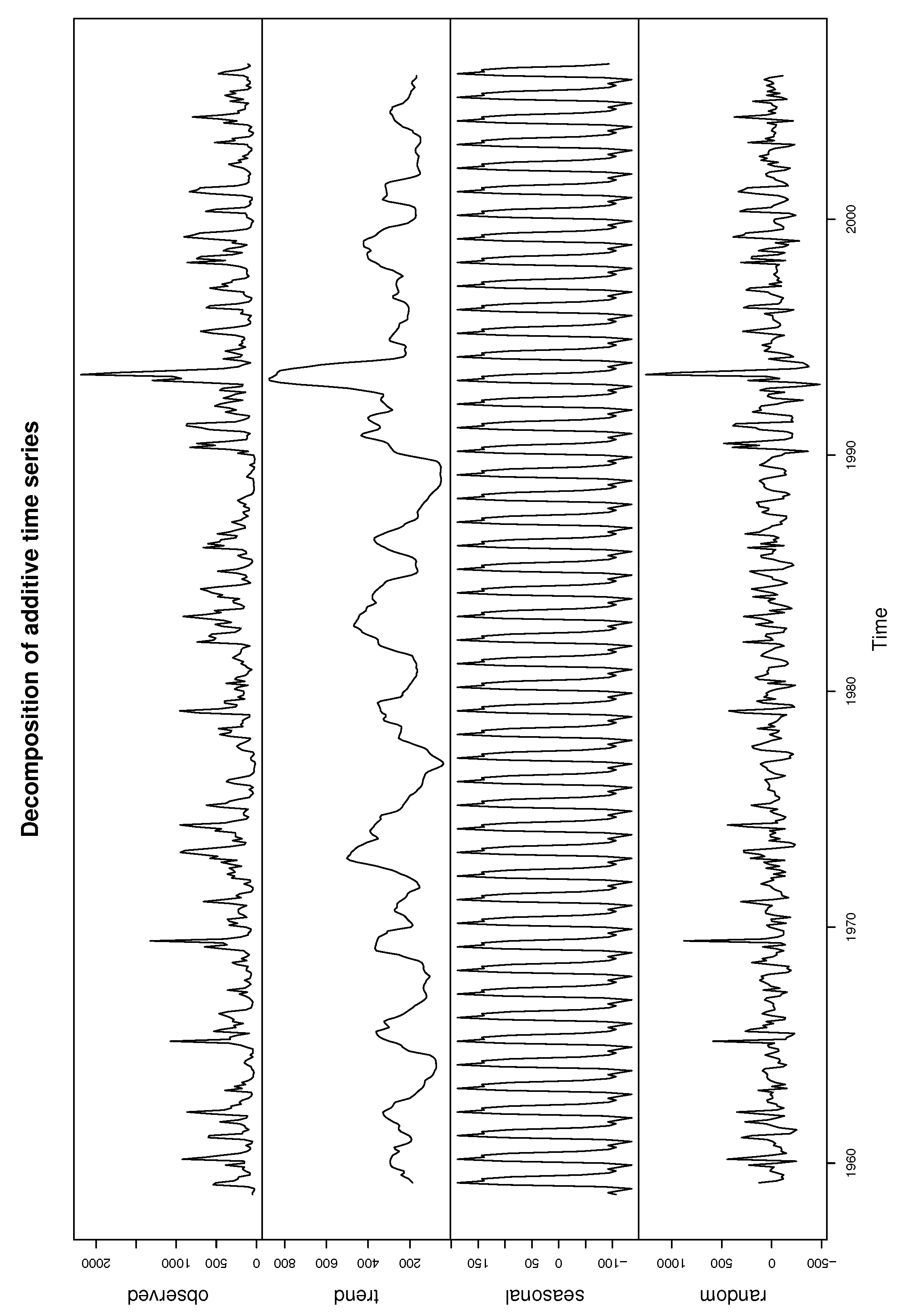
Figure 10 plots the time series of the Iowa river monthly flow. It shows that the data have significant annual periodicity and strong seasonal effects, so the single threshold is inappropriate. It is significant to develop the regression structure for the threshold. Figure 8 decomposed the time series data into a trend, seasonal and random components using moving averages. The seasonality of Iowa river flow can be observed in Figure 11.

Figure 10.
Time series of the Iowa river monthly flow.
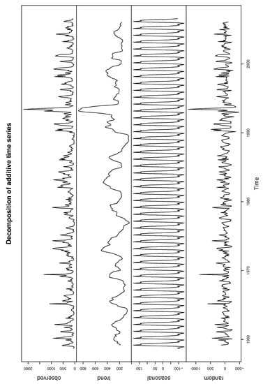
Figure 11.
Decomposition of additive time series for Iowa river monthly flow.
As shown in [1,16], the seasonality obviously present in environment data can be incorporated into the model through trigonometric functions. The effect of the season is in most cases well captured by the sine wave and cosine wave. Since the Iowa river flow data is in monthly time series units, we give two covariates and in the regression structure of the parameters u, , and , which can capture the seasonal behavior of the data, the m is the month. For the regression coefficients parameters of , and , we consider the prior distribution as the simulation part in Section 4. For the regression coefficients parameters of u, we consider the prior distribution , and .
Table 4 shows the estimates for the regression coefficients and the respective credibility intervals. We can see that the values of all the coefficients behave around intervals in which the value zero is not included, thus presenting significant significance for the estimation of their respective parameters. It means that the seasonal covariates and presented significant effects. For the regression coefficients of parameter , we note the result of is negative, which means that the data has the light tail behavior. With the estimation of the regression coefficients, we can see how the parameters of the DPMW-PPR distribution behave over the months.
Table 4.
Estimates and credibility interval for the regression coefficients of the Iowa river monthly flow.
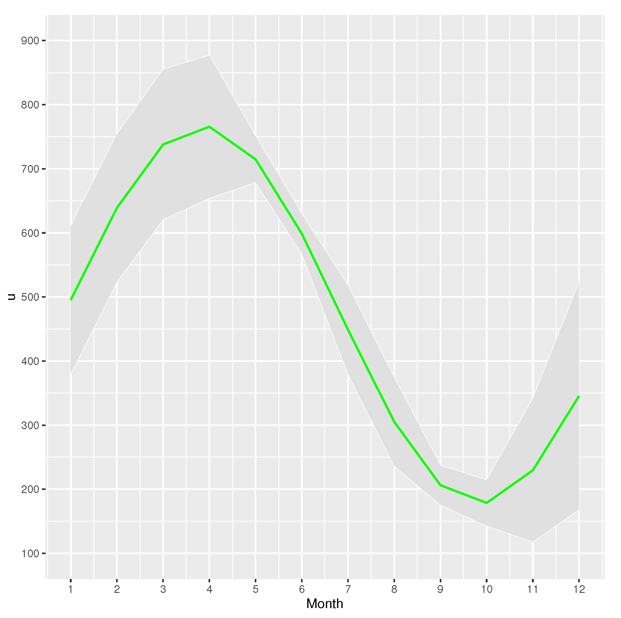
In Figure 12, we can see the estimate of threshold u varying over the twelve months. It illustrates that the estimated values of the threshold u increased significantly from the October of the previous year to April of the current year, revealing the high values for the threshold between March to May of the year. The estimated values of the threshold u decreased significantly from April to October and the estimate of the threshold reaches its peak in April and falls to the lowest value in October.

Figure 12.
Parameter u varying over time for the data of Iowa river flow. The green line is the estimate of the parameter u. The shaded area is the confidence interval of the estimates.
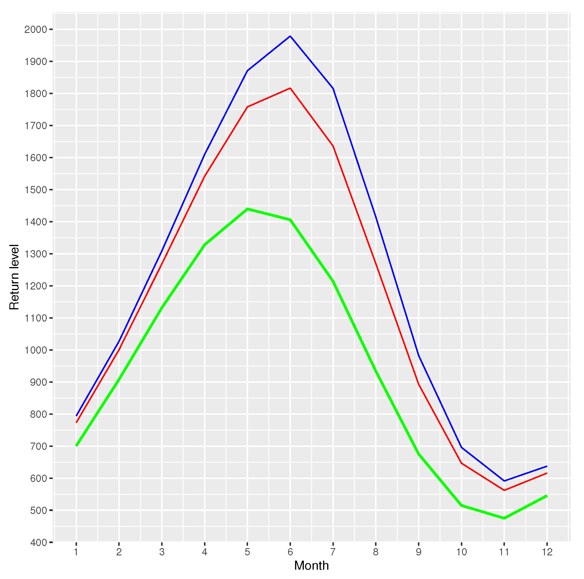
In Figure 13, we show the return levels for every 10, 50 and 100 years periods. For the expected return level, the month of May is the month that presents the highest level of return, with values of 1439.791 m/s for every 10 years periods, the month of June is the month that presents the highest level of return, with values of 1816.659 m/s for every 50 years periods and 1978.948 m/s for every 100 years periods, respectively. The return levels are lowest in the months of October with values of 474.8953 m/s for every 10 years periods, 562.0131 m/s for every 50 years periods and 591.2955 m/s for every 100 years periods, respectively.
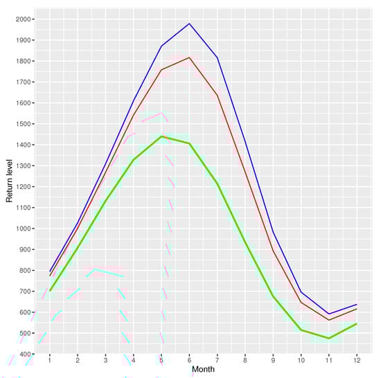
Figure 13.
Return levels expected every 10, 50 and 100 years. Green: expected return every 10 years; red: expected return every 50 years; blue: expected return every 100 years.
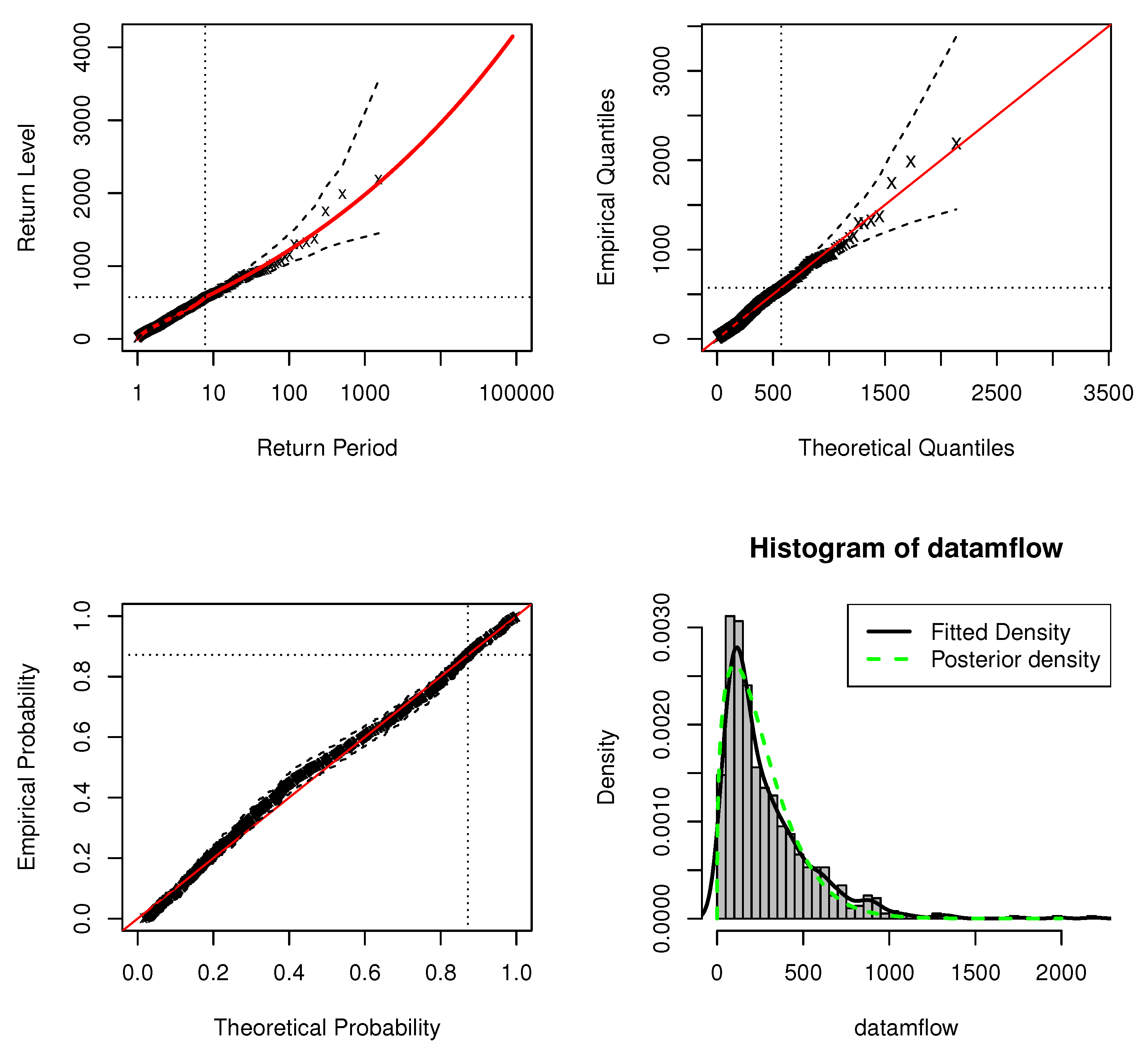
Figure 14 shows the standard model fit diagnostics for the application of the DPMW-PPR model. Neither the probability plot nor the quantile plot causes doubt in the validity of the fitted model: each set of plotted points is near-linear. We have the adjustment of expected return levels in the original series of the Iowa river flow. The return level curve also provides a satisfactory representation of the empirical estimates. Finally, the corresponding density estimate seems consistent with the histogram of the data. Consequently, all four diagnostic plots lend support to the fitted DPMW-PPR model of the Iowa river monthly flow.
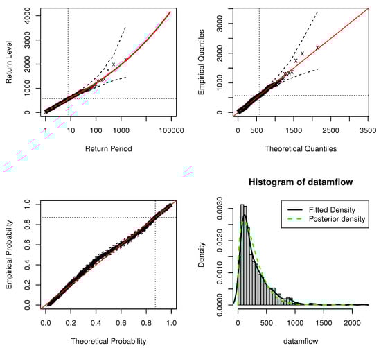
Figure 14.
Standard model fit diagnostics for the DPMW-PPR model fitted to the Iowa River monthly flow. (The top left corner is the return level plot, the top right corner is the quantile plot, the bottom left corner is the probability plot, and the bottom right corner is the density plot).
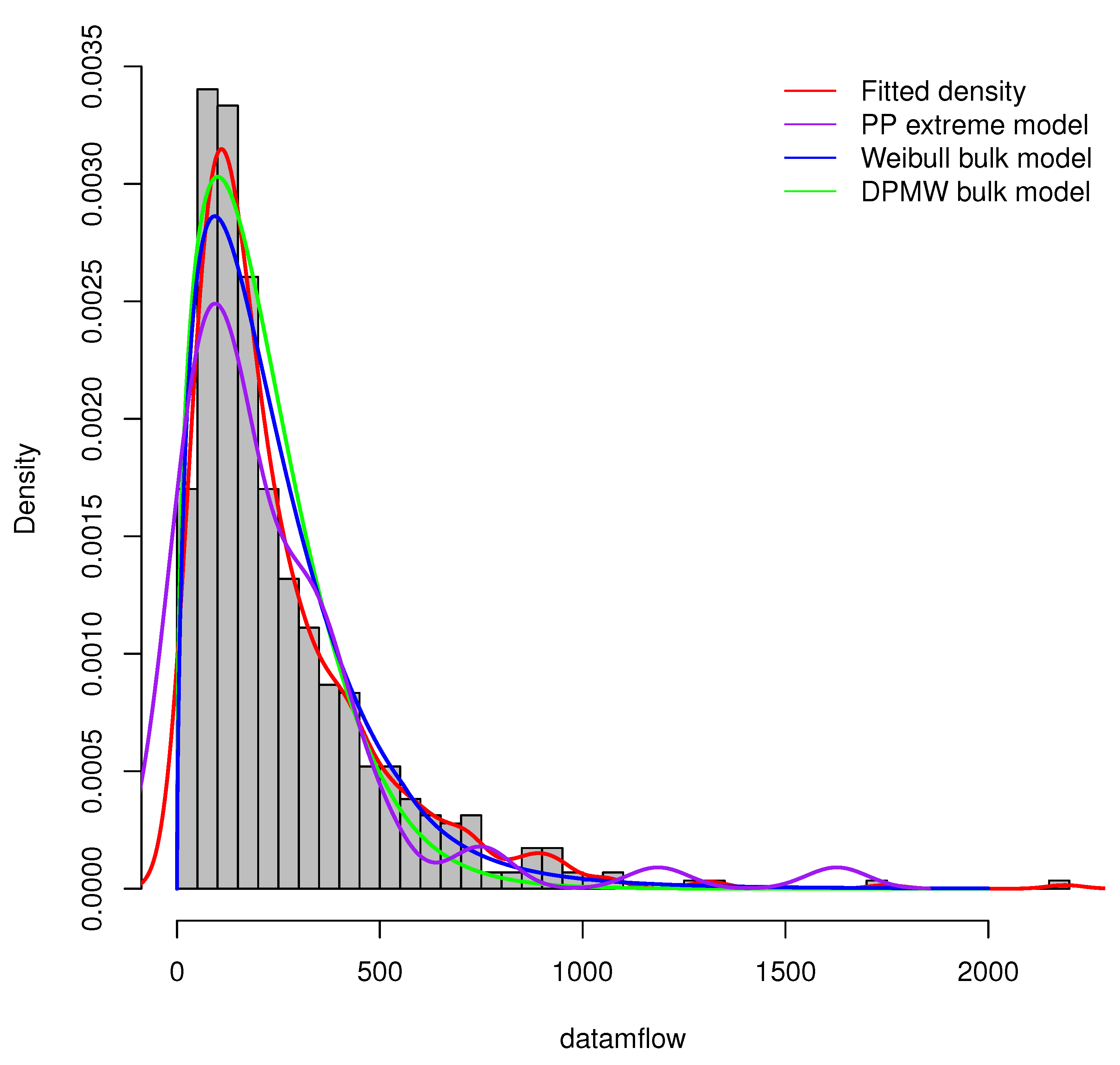
Furthermore, we compare the proposed model (DPMW-PPR) with the Point Process (PP) extreme value model and the Weibull mixture Point Process (WMPP) extreme model [3]. Figure 15 shows the true fitted density and the posterior density of the above three models with the Iowa River monthly flow data, respectively. Obviously, our proposed model is superior to the other two models.
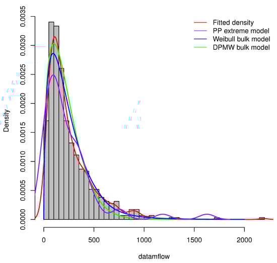
Figure 15.
The posterior density plot for three models (the DPMW-PPR model, the PP extreme value model and the WMPP extreme model) fitted to the Iowa River monthly flow data. The red line shows the true density function, the green line, the blue line and the purple line are the posterior density function of the DPMW-PPR model, the WMPP extreme model and the PP extreme value model, respectively.
5.2. The Daily Flow in the Patuxent River
The Patuxent river is the longest river contained entirely within Maryland in the United States, and along its length, changes from a slow-moving stream to a wide tidal estuary that empties into the Chesapeake Bay near the southernmost point of Maryland’s Western Shore. The Patuxent river daily flow observations from the USGS stream gage station 01594440 near Bowie, Maryland. The data used in this subsection is the daily flow data (in cubic meters per second) for the Patuxent river for the period from the prior 1 January 2005 to 30 December 2014 and data missing for very few dates. The sample size of this data set is . The Patuxent river data set is provided by National Water Information System (Available online: https://waterdata.usgs.gov/md/nwis/dvstat (accessed on 21 November 2021).
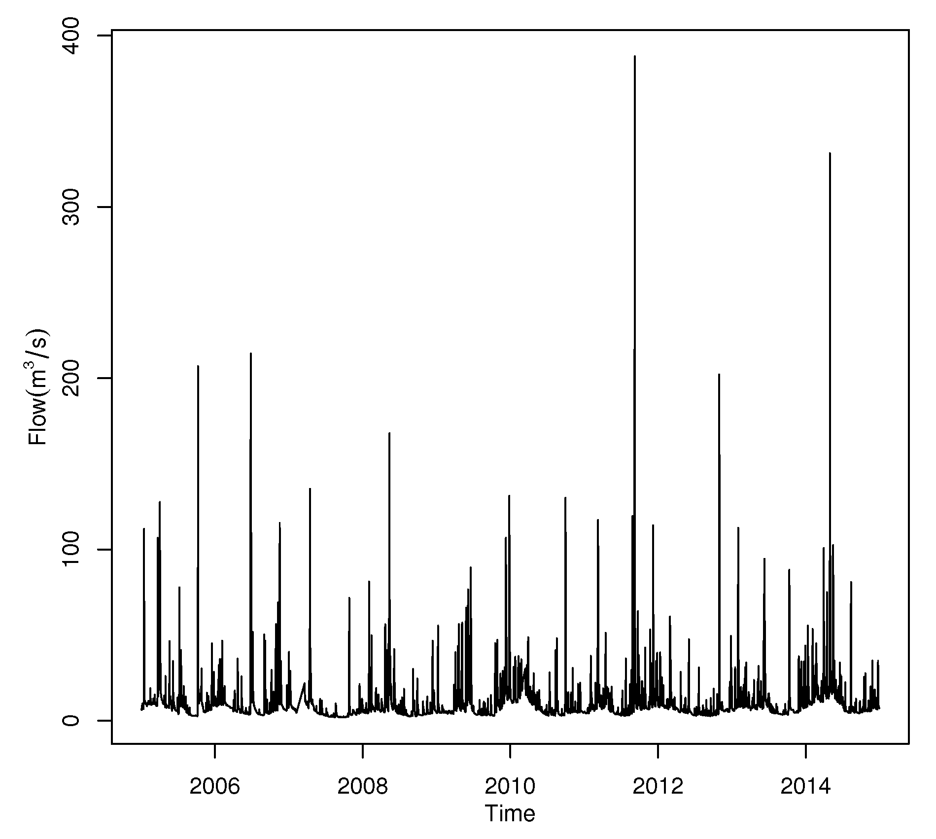
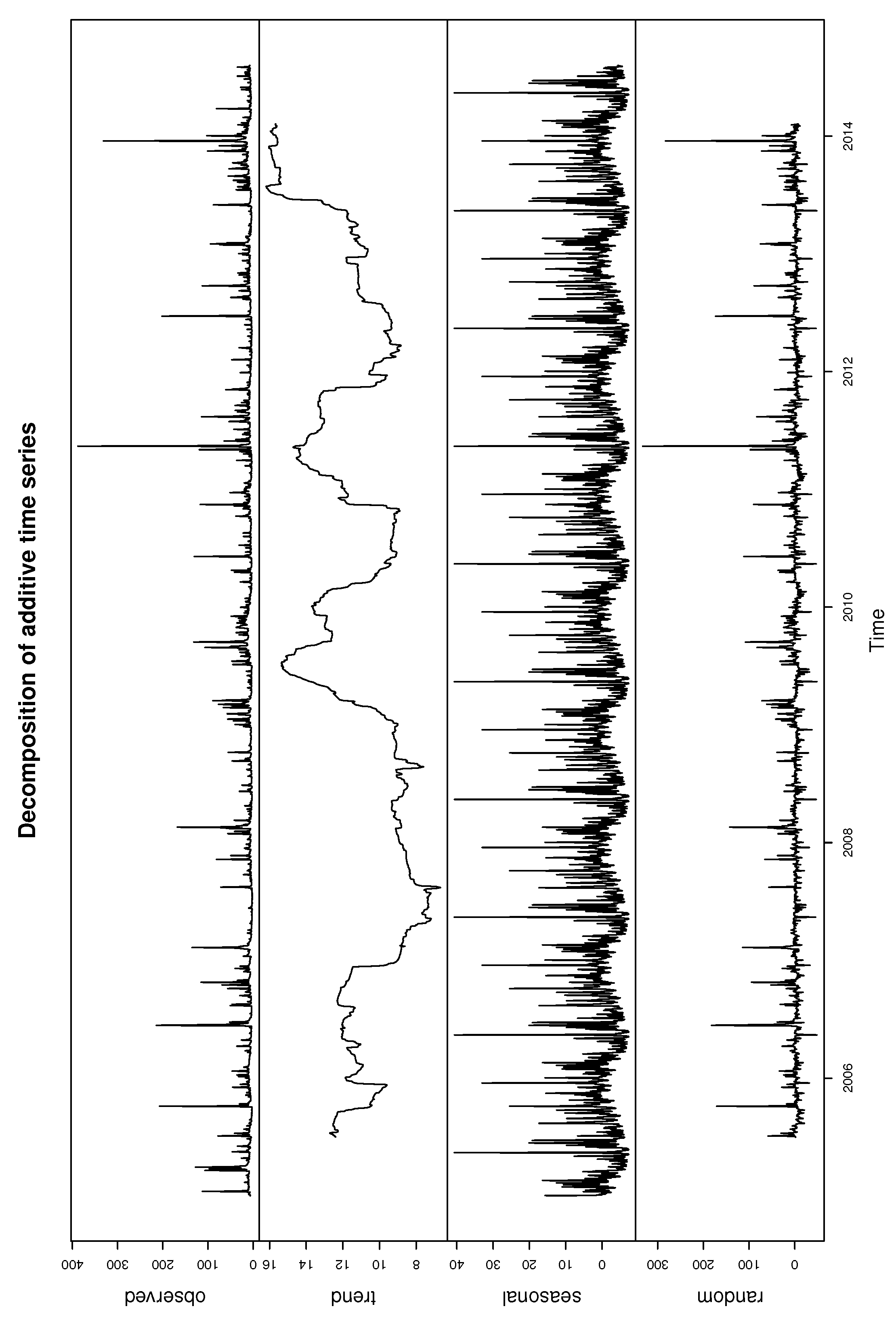
Figure 16 plots the time series of the Patuxent river daily flow. The data has significant annual periodicity and strong seasonal effects. It is significant to develop the regression structure for the threshold. In Figure 17, we decomposed the time series data and the seasonality of Patuxent river flow can be observed from the figure.

Figure 16.
Time series of the Patuxent river daily flow.

Figure 17.
Decomposition of additive time series for Patuxent river daily flow.
Since the Patuxent river flow data is in daily time series units, we give two covariates and in the regression structure of the parameters u, , and , where t is the data order. We consider the prior distribution of regression coefficients as Section 5.1.
Table 5 shows the estimates for the regression coefficients and the respective credibility intervals. For the regression coefficients of shape parameter , we see that the coefficients and are not significant, showing that there is no seasonality for the shape parameter. We also note that the parameter is positive, indicating that the data have a long tail distribution. Regarding the parameters and and the threshold u, all regression coefficients are significant, we consider that the seasonal covariates and both presented significant effects for this parameters.
Table 5.
Estimates and credibility interval for the regression coefficients of the Patuxent river daily flow.
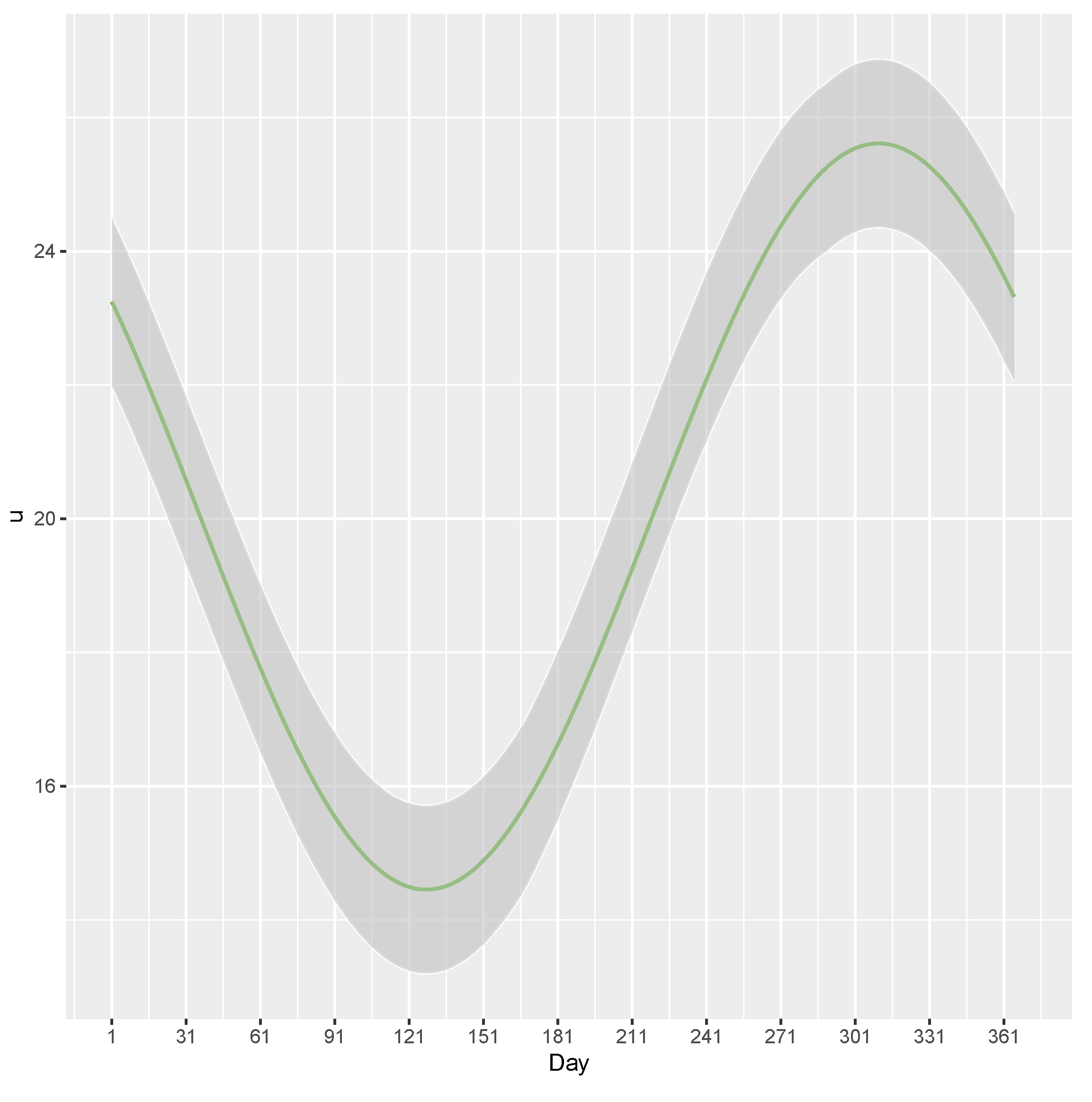
In Figure 18, we can see the estimate of threshold u varying over 365 days. It illustrated that the estimated values of the threshold u decreased significantly from around the 308th day of the previous year to around the 129th day of the current year and the estimate of the threshold increased dramatically from around the 129th day of the year to around the 308th day of the year, the estimate of threshold falls with the lowest values on about the 129th of the year and reaches its peak on about the 308th of the year.
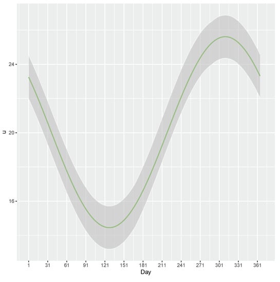
Figure 18.
Parameter u varying over time for the data of Patuxent river flow. The green line is the estimate of the parameter u. The shaded area is the confidence interval of the estimates.
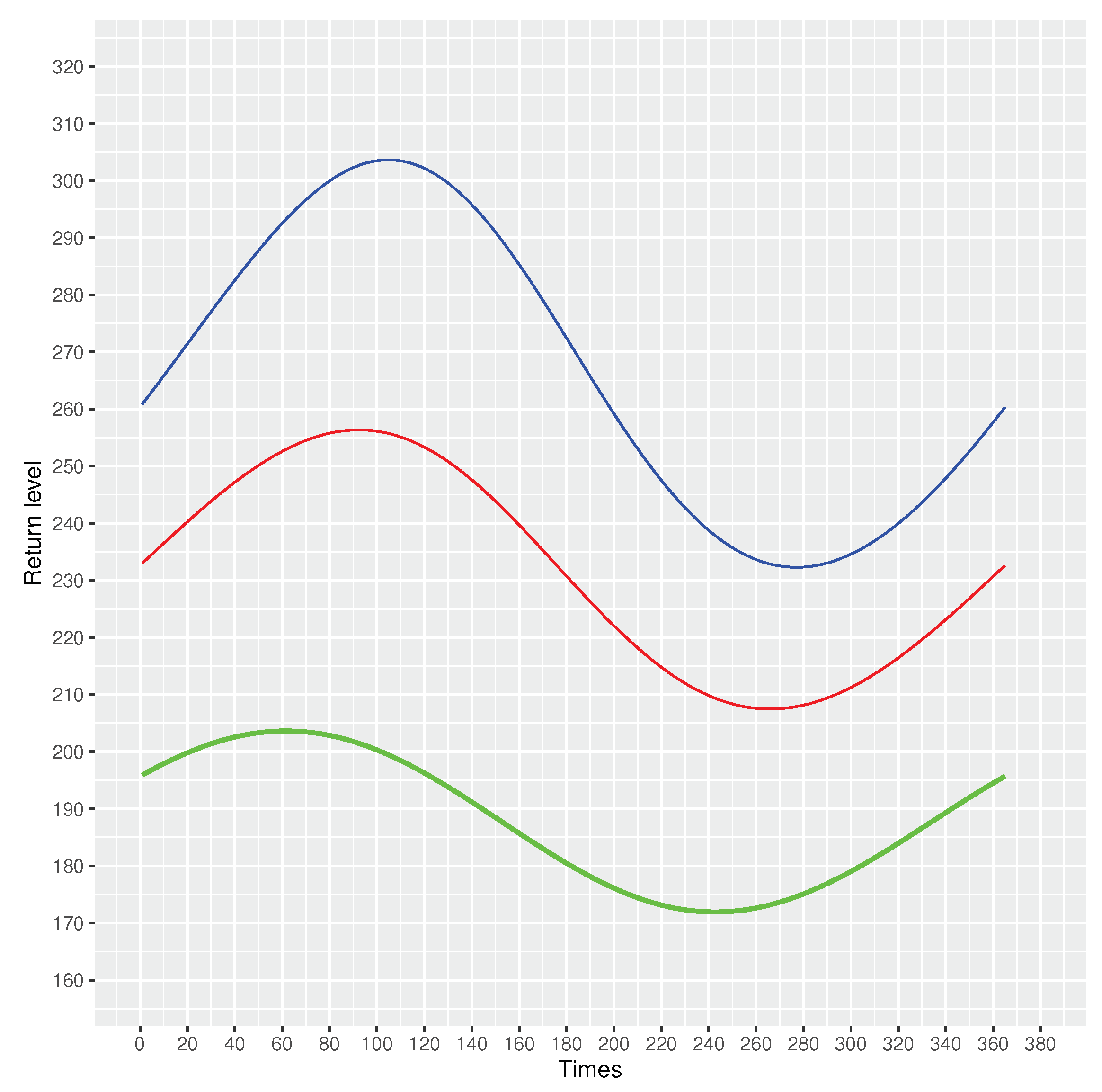
In Figure 19, we show the return levels for every 10, 50 and 100 years periods. For the expected return level, the highest level of return is 203.6169 m/s for every 10 years periods, 256.3437 m/s for every 50 years periods and 303.6306 m/s for every 100 years periods. The lowest level of return is 171.9141 m/s for every 10 years periods, 207.4655 m/s for every 50 years periods and 232.2825 m/s for every 100 years periods.
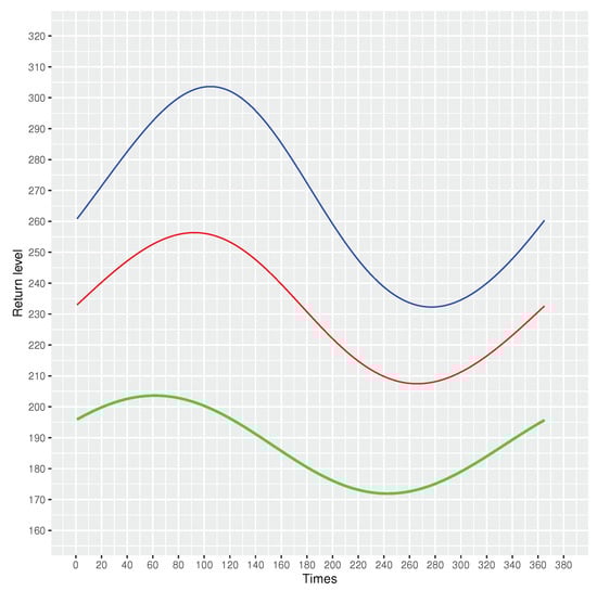
Figure 19.
Return levels expected every 10, 50 and 100 years for Patuxent river daily flow. Green: expected return every 10 years; red: expected return every 50 years; blue: expected return every 100 years.
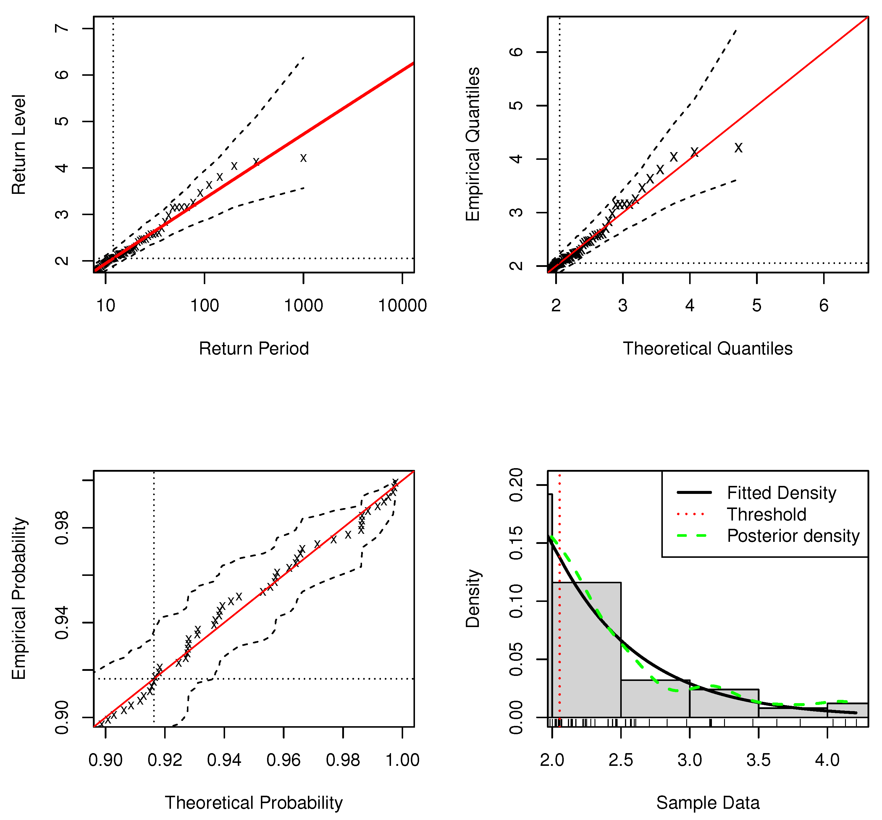
Figure 20 shows the standard model fit diagnostics for the application of the DPMW-PPR model. Neither the probability plot nor the quantile plot causes doubt in the validity of the fitted model: each set of plotted points is near-linear. We have the adjustment of expected return levels in the original series of the Patuxent river flow. Since the shape parameter , the return level plot is concave. The return level curve also provides a satisfactory representation of the empirical estimates. Finally, the corresponding density estimate seems consistent with the histogram of the data and the posterior distribution has a heavy tail which provides a satisfactory representation of the empirical estimates. Consequently, all four diagnostic plots lend support to the fitted DPMW-PPR model of the Patuxent river daily flow.

Figure 20.
Standard model fit diagnostics for the DPMW-PPR model fitted to the Patuxent river daily flow. (The top left corner is the return level plot, the top right corner is the quantile plot, the bottom left corner is the probability plot, and the bottom right corner is the density plot).
Different from the general extreme value model, we model all data, not only those belonging to the tail. With the DPMW distribution under the threshold, the proposed model works well even in the absence of prior distribution and small sample sizes. The regression structure for the PP model parameters explains the behavior of the time series. Furthermore, we compare the proposed model (DPMW-PPR) with the Point Process (PP) extreme value model and the Weibull mixture Point Process (WMPP) extreme model which combined the Weibull distribution in the bulk part and the Point Process extreme value model in the tail [3]. Figure 21 shows the true fitted density and the posterior density of the above three models fitted to the Patuxent river daily flow, respectively. Obviously, our proposed model is superior to the other two models.
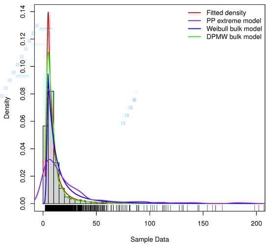
Figure 21.
The posterior density plot for three models (the DPMW-PPR model, the PP extreme value model and the WMPP extreme model) fitted to the Patuxent river daily flow. The red line shows the true density function, the green line, the blue line and the purple line are the posterior density function of the DPMW-PPR model, the WMPP extreme model and the PP extreme value model, respectively.
6. Conclusions
In this paper, we consider a new extreme mixture model, which includes a Dirichlet process mixture of Weibull distribution below the threshold and the point process extreme model for the upper tail. The model developed the addition of a regression structure for the estimation of the PP extreme model parameters based on the Bayesian approach, the prior distributions will not be attributed directly to the extreme parameters, but to the coefficients of their linear structure. With the Dirichlet process mixture of Weibull distribution, the proposed model works well even in the absence of prior distribution and small sample sizes. The regression structure for the PP model parameters explains the behavior of the time series. The model is shown in both simulation and environmental data to demonstrate performance in extrapolating extreme events.
Author Contributions
Conceptualization, Y.W.; methodology, Y.W.; software, Y.W.; validation, Y.W. and X.L.; formal analysis, Y.W. and X.L.; writing—original draft preparation, Y.W.; writing—review and editing, Y.W.; supervision, X.L. All authors have read and agreed to the published version of the manuscript.
Funding
This research was funded by Natural Science Foundation of China (grant no. 61374183) and Postgraduate Research & Practice Innovation Program of Jiangsu Province (grant no. KYCX22_0322).
Data Availability Statement
Not applicable.
Acknowledgments
The authors would like to thank the editors and reviewers for providing useful comments and suggestions to improve the quality of this article.
Conflicts of Interest
The authors declare no conflict of interest.
References
- Coles, S. An Introduction to Statistical Modeling of Extreme Values; Springer: London, UK, 2001. [Google Scholar]
- Coles, S.; Tawn, J. A Bayesian analysis of extreme rainfall data. J. R. Stat. Soc. Ser. C-Appl. Stat. 1996, 45, 463–478. [Google Scholar]
- MacDonald, A.; Scarrott, C.J.; Lee, D.; Darlow, B.; Reale, M.; Russell, G. A flexible extreme value mixture model. Comput. Stat. Data Anal. 2011, 55, 2137–2157. [Google Scholar]
- Pickands, J. The two dimensional Poisson process and extremal processes. J. Appl. Probab. 1971, 8, 745–756. [Google Scholar]
- Pickands, J. Statistical inference using extreme order statistics. Ann. Stat. 1975, 3, 119–131. [Google Scholar]
- Northrop, P.J.; Attalides, N.; Jonathan, P. Cross-validatory extreme value threshold selection and uncertainty with application to ocean storm severity. J. R. Stat. Soc. Ser. C-Appl. Stat. 2017, 66, 93–120. [Google Scholar]
- Frigessi, A.; Haug, O.; Rue, H. A dynamic mixture model for unsupervised tail estimation without threshold estimation. Extremes 2002, 5, 219–235. [Google Scholar]
- Behrens, C.N.; Lopes, H.F.; Gamerman, D. Bayesian analysis of extreme events with threshold estimation. Stat. Model. 2003, 4, 227–244. [Google Scholar]
- Kottas, A. Nonparametric Bayesian survival analysis using mixtures of Weibull distributions. J. Stat. Plan. Infer. 2006, 136, 578–596. [Google Scholar]
- Ferguson, T. A Bayesian Analysis of Some Nonparametric Problems. Ann. Stat. 1973, 1, 209–230. [Google Scholar]
- Antoniak, C.E. Mixture of Dirichlet process with applications to Bayesian Nonparametric problems. Ann. Stat. 1974, 2, 1152–1174. [Google Scholar]
- Hanson, T.E. Modelling censoring lifetime data using a mixture of gamma baselines. Bayesian Anal. 2006, 3, 575–593. [Google Scholar]
- Patino, F. A semi-parametric Bayesian extreme value model using a Dirichlet process mixture of gamma densities. J. Appl. Stat. 2015, 42, 267–280. [Google Scholar]
- Smith, R. Maximum likelihood estimation in a class of non-regular cases. Biometrika 1985, 72, 67–90. [Google Scholar]
- Wadsworth, J.L.; Tawn, J.A.; Jonathan, P. Accounting for choice of measurement scale in extreme value modeling. Ann. Appl. Stat. 2010, 4, 1558–1578. [Google Scholar]
- Nascimento, F.F.; Gamerman, D.; Lopes, H.F. Regression models for exceedance data via the full likelihood. Environ. Ecol. Stat. 2011, 18, 495–512. [Google Scholar]
- Nascimento, F.F.; Azevedo, A.; Ferraz, V.R. Regression models to dependence for exceedance. J. Appl. Stat. 2020, 16, 3048–3059. [Google Scholar]
- Chaves-Demoulin, V.; Davison, A.C. Generalized additive modelling of sample extremes. J. R. Stat. Soc. Ser. C-Appl. Stat. 2005, 54, 207–222. [Google Scholar]
- Nascimento, F.F.; Assuncao, A. Regression models for change point data in extremes. Braz. J. Probab. Stat. 2021, 35, 85–100. [Google Scholar]
- Lima, S.R.; Nascimento, F.F.; Ferraz, V.R.S. Regression models for time-varying extremes. J. Stat. Comput. Simul. 2018, 88, 235–249. [Google Scholar]


Publisher’s Note: MDPI stays neutral with regard to jurisdictional claims in published maps and institutional affiliations. |
© 2022 by the authors. Licensee MDPI, Basel, Switzerland. This article is an open access article distributed under the terms and conditions of the Creative Commons Attribution (CC BY) license (https://creativecommons.org/licenses/by/4.0/).