Abstract
Some matrix-splitting iterative methods for solving systems of linear equations contain parameters that need to be specified in advance, and the choice of these parameters directly affects the efficiency of the corresponding iterative methods. This paper uses a Bayesian inference-based Gaussian process regression (GPR) method to predict the relatively optimal parameters of some HSS-type iteration methods and provide extensive numerical experiments to compare the prediction performance of the GPR method with other existing methods. Numerical results show that using GPR to predict the parameters of the matrix-splitting iterative methods has the advantage of smaller computational effort, predicting more optimal parameters and universality compared to the currently available methods for finding the parameters of the HSS-type iteration methods.
Keywords:
Gaussian process regression; matrix-splitting iterative method; data-driven method; HSS iteration method; LHSS iteration method; NHSS iteration method; SHSS iteration method; SHSS-SS iteration method; MHSS iteration method; MSNS iteration method; linear systems MSC:
15A24; 65F45
1. Introduction
Solving linear equations is one of the most fundamental topics in matrix computation, and with the development of science and technology, many important problems in the natural sciences and engineering can often be reduced to the following linear equation:
where , is a large sparse non-Hermitian and positive definite matrix.
There are many powerful matrix-splitting iterative methods for solving systems of linear equations, such as the successive over-relaxation (SOR) method [1], the symmetric SOR (SSOR) method [2], the accelerated over-relaxation (AOR) method [3] and the symmetric AOR (SAOR) method [4]. Many researchers have applied them to different problems and made some improvements [5,6,7,8]. Considering the specificity of the problem and solving Equation (1) more efficiently, many new matrix-splitting iterative methods have been proposed. Bai et al. offered the Hermitian and skew-Hermitian splitting (HSS) method and the inexact HSS method [9]. To improve the efficiency of the HSS method, Bai et al. proposed the preconditioned HSS (PHSS) [10]. Due to the promising performance of the HSS method, some HSS-type iteration methods were presented. These methods can be mainly divided into the following two forms. The first one is accelerated HSS-type methods. Such as the generalized HSS method [11], the lopsided HSS (LHSS) method [12], the generalized PHSS method [13], the asymmetric HSS method [14] and the new HSS (NHSS) method [15]. In addition, Yang et al. offered the minimum residual HSS method [16] by applying the minimum residual technique to the HSS method and Li et al. [17] proposed the single-step HSS (SHSS) method. Based on the shift-splitting method and the SHSS method, Li et al. established the SHSS-SS method [18].
Apart from the accelerated HSS-type methods, some other HSS-type methods focused on the applications to different kinds of problems. Such as the saddle-point problems [19,20,21,22,23,24], solving the matrix equation [25,26,27,28,29,30,31,32], and solving the complex symmetric linear systems [33,34,35] and the nonlinear systems [36,37].
These iteration methods contain splitting parameters that need to be specified in advance. At present, there are three main methods of selecting the splitting parameters. The first is obtaining relatively optimal parameters by traversing or experimenting within some intervals [26,38,39]. The advantage of this traversal method is that it can obtain relatively accurate optimal parameters, but it requires large amount of calculation and consumes a lot of extra time, especially when the dimension of the coefficient matrix is large. The second is estimating optimal parameters through theoretical analysis [40,41]. Some researchers find optimal parameters by minimizing the spectral radius of the iterative matrix. However, solving this optimization problem is very difficult in theoretical analysis and practical computation. Bai et al. [42] proposed an accurate formula for computing the optimal parameters of the HSS method by directly minimizing the spectral radius of the iterative matrix, but the coefficient matrix is a two-by-two matrix or a two-by-two block matrix with specific forms. Some researchers find quasi-optimal parameters by minimizing the upper bound of the spectral radius of the iterative matrix of some iteration methods [9,12,17,18]. By a reasonable and simple optimization principle, Chen [43] proposed an accurate estimate to the optimal parameter of the HSS iteration method. Huang [44] and Yang [45] estimated the optimal parameters of the HSS method by solving a cubic polynomial equation and a quartic polynomial equation, respectively. Huang [46] proposed variable-parameter HSS methods and the parameter in it updated at each step of the iteration. The above theoretical methods contain the following limitations. First, the method is only available case by case, which means it is less universal. Second, the method needs to compute the maximum or the minimum eigenvalues of the matrix, but this is time-consuming work. Jiang et al. [47] proposed the third estimation method, the Bayesian inference-based Gaussian process regression (GPR) method, to predict the optimal parameters in some alternating direction iterative methods. This method uses a training set to learn a mapping between the dimension of linear systems and relatively optimal splitting parameters.
The choice of splitting parameters can greatly affect the efficiency of the HSS-type iteration methods [47,48], which makes the parameter selection of great importance. For computing the splitting parameters of the HSS-type iteration methods, to overcome the limitations of the traversal method and the theoretical methods, we use the GPR method to predict the splitting parameters of some HSS-type iteration methods. The main contributions of this work are:
- We apply the GPR method for the prediction of optimal splitting parameters of some HSS-type methods, which is a new application.
- We provide extensive numerical experiments to compare the prediction performance of the GPR method with the traversal method and the theoretical methods.
The results of numerical experiments show that: comparing to the traversal method, the GPR method can predict almost the same parameters as the traversal method does but with less computational effort; comparing to the theoretical method, the GPR method can predict better optimal parameters than the theoretical method and is more universal (unlike the theoretical method available case by case, the GPR method is suitable for all the HSS-type iteration methods tested). Moreover, the theoretical methods need to compute the maximum or the minimum eigenvalues (or singular values) of the matrix but this is a time-consuming work when the dimension of the matrix is large and the GPR method overcomes this limitation.
The rest of the paper is organized as follows. In Section 2, we present Gaussian process regression method based on Bayesian inference. In Section 3, we present the iteration scheme of some HSS-type iteration methods, the corresponding convergence conditions and the theoretical methods for estimating the relatively optimal splitting parameters. In Section 4, we illustrate the efficiency of the GPR method by numerical experiments. Finally, in Section 5, we include some concluding remarks and prospects.
Throughout the paper, the sets of complex and real matrices are denoted by and , respectively. If , let ,,,, denote the transpose, inverse, conjugate transpose, the Euclidean norm and Frobenius norm of X, respectively. The notations , , denote the eigenvalue set, singular value set and spectral radius of X, respectively. The symbol ⊗ denotes the Kronecker product. I represents the identity matrix.
2. Gaussian Process Regression Method
In this section, we present a Gaussian process regression method based on Bayesian inference. Gaussian process regression is an application of non-parametric Bayesian estimation to regression problems and has a wide range of applications in the field of machine learning.
2.1. Bayesian Inference
Bayesian inference is a method that infers the population distribution or the characteristic number of the population according to the sample information and the prior information. Prior information is some information about statistical problems before sampling. Taking inferrance of the distribution of an unknown quantity as an example, Bayesian inference believes that can be regarded as a random variable before obtaining the sample information, so it can be described by a probability distribution and this distribution is a prior distribution. After obtaining the samples, the population distribution, samples and the prior distribution are combined by Bayesian formula to obtain a new distribution about the unknown quantity , which is a posterior distribution. We can find that the process of Bayesian inference is essentially the process of updating prior information through sample information.
The Bayesian inference-based Gaussian process regression method is Bayesian inference with Gaussian process as a prior distribution. The definition of Gaussian process is given below.
Definition 1.
Gaussian process (GP) is a collection of random variables and for any finite subset of T, follows the joint Gaussian distribution.
In our question, we expect to obtain a mapping from the dimension of linear systems to relatively optimal splitting parameters, so that for each given dimension , the mapping can output the corresponding relatively optimal splitting parameter . To this end, this paper uses the GPR to fit this mapping .
2.2. Model Building
Following the steps of Bayesian inference, firstly, we give prior information. For each given , the corresponding optimal splitting parameter is a random variable, and we denote as to reflect the correspondence between and n. Considering that, in general, the observed would be polluted by addition noise, the observed may not be exactly equal to . It is
where is the addition noise and we assume that follows a Gaussian distribution with zero mean and variance , i.e., . The desirable range of is . In this work, we take . We also assume that are independent of each other. Obviously, our task is to obtain .
Considering random process and assuming this process is a GP, we have
where and denote mean function and covariance function of the GP , respectively. Once and have been determined, the GP is also determined. The selection of and is shown in Section 2.3.
Next, we obtain sample information. Assume that we have a training set where is an input–output pair. is the dimension of the coefficient matrix and is the optimal splitting parameter in a matrix-splitting iterative method. Obviously, the training set is the sample information. According to the prior information, follows the joint Gaussian distribution, i.e.,
Or equally,
where . From Equation (2), the distribution of the corresponding observed is
where is a d-order identity matrix.
Finally, we can update the prior information by using the sample information. That is to say, to predict new dimensional vector , we can obtain the distribution of the optimal splitting parameters corresponding to , i.e., the conditional distribution , where . According to the prior information, the sample and predicted value of follow the joint Gaussian distribution. From Equation (3), we have
To obtain the conditional distribution from Equation (4), we have the following theorem [49].
Theorem 1.
Let and be jointly Gaussian random vectors, i.e.,
then the marginal distribution of and the conditional distribution of given by are
From Theorem 1, we have
where
For the predicted value , one can use the mean value of the above Gaussian distribution as its estimated value, i.e., . Now, we have successfully obtained the function , and denoted the independent variable of by ; then, .
2.3. Model Selection
In this section, we determine and . In this work, we let , other ways can refer to [49]. For covariance function, the exponential kernel function is
where is the hyperparameter. In this work, maximum likelihood estimation is used to select the values of the hyperparameter . Specifically, when we have a training set , the likelihood function L of can be derived as
The optimal hyperparameter is .
In practice, to avoid a large amount of calculation, we generally produced the training set from a set of small-scale systems.
3. Matrix-Splitting Iterative Methods
In this section, we recall some matrix-splitting iteration methods, including the HSS method, the NHSS method, the LHSS method, the SHSS method, the SHSS-SS method, the MHSS method and the MSNS method. We mainly focus on their iterative schemes, convergence and theoretical methods involving estimating optimal splitting parameters.
3.1. Matrix-Splitting Methods for Non-Hermitian Positive Definite Linear Systems
For the HSS method, the NHSS method, the LHSS method, the SHSS method and the SHSS-SS method, they all split A into Hermitian and skew-Hermitian parts. i.e.,
3.1.1. HSS Iteration Method
The scheme of HSS iteration [9] is as follows.
Definition 2.
Given an initial guess , for until converges, compute
where α is a given positive constant.
For the convergence property of the HSS iteration, we have the following theorem [9]:
Theorem 2.
Let A in Equation (5) be a positive definite matrix, the matrixes be defined in the same way as Equation (6) and let α be a positive constant. Then, the iteration matrix of the HSS iteration is given by
and its spectral radius is bounded by
where is the spectral set of the matrix M. Therefore, it holds that
i.e., the HSS iteration converges to the unique solution of the Equation (5).
Equation (7) provides a theoretical method to estimate the optimal splitting parameter, that is, by minimizing the upper bound of the spectral radius of the iteration matrix of the HSS iteration to obtain the quasi-optimal splitting parameter , and it is shown by the following theorem [9].
Theorem 3.
The conditions are the same as Theorem 2: let and be the minimum and the maximum eigenvalues of the matrix M, respectively. Then
The HSS iteration needs to solve two linear systems with coefficient matrices and , which is costly and impractical. An approach to overcome this disadvantage is to solve two subproblems iteratively and this result is the inexact HSS (IHSS) iteration method.
Definition 3.
Given an initial guess , for until converges,
- 1.
- Approximately solve by employing an inner iteration (e.g., the CG method), such that the residual satisfiesand then compute ;
- 2.
- Approximately solve ) by employing an inner iteration (e.g., some Krylov subspace method), such that the residual satisfiesand then compute , here α is a given positive constant.
The convergence property and the choice of the tolerance and can refer to [9].
3.1.2. NHSS Iteration Method
The scheme of NHSS [15] iteration is as follows.
Definition 4.
Given an initial guess , for until converges, compute
where α is a given positive constant.
For the convergence property of the NHSS iteration, we have the following theorem [15]:
Theorem 4.
Let A in Equation (5) be a positive definite and normal matrix; the matrixes be defined in the same way as Equation (6) and let α be a positive constant. Then, the iteration matrix of the NHSS iteration is
The spectral radius is bounded by
where is the maximum singular value of the matrix N and is the minimum eigenvalue of the matrix M. Moreover, if , then
i.e., the NHSS iteration converges to the unique solution of Equation (5).
Equation (8) provides a theoretical method to estimate the optimal splitting parameter, that is, by minimizing the upper bound of the spectral radius of the iteration matrix of the NHSS iteration to obtain the quasi-optimal splitting parameter , and it is given by Theorem 5 [15].
Theorem 5.
The conditions are the same as Theorem 4; then, the quasi-optimal splitting parameter of the NHSS iteration is
3.1.3. LHSS Iteration Method
The scheme of LHSS iteration [12] is as follows.
Definition 5.
Given an initial guess , for until converges, compute
where α is a given positive constant.
For the convergence property of the LHSS iteration, we have the following theorem [12]:
Theorem 6.
By minimizing the upper bound of the spectral radius of the iteration matrix of the LHSS iteration in Equation (9), we can obtain the quasi-optimal splitting parameter using Theorem 7 [12].
Theorem 7.
The conditions are the same as Theorem 6: let and be the minimum and the maximum eigenvalues of the matrix M, respectively. Let be the maximum singular value of the matrix N. Then
To improve the efficiency of the LHSS iteration method, we have the following ILHSS iteration method.
Definition 6.
Given an initial guess , for until converges,
- 1.
- Approximately solve by employing an inner iteration (e.g., the CG method), such that the residual satisfiesand then compute ;
- 2.
- Approximately solve ) by employing an inner iteration (e.g., a Krylov subspace method), such that the residual satisfiesand then compute , where α is a given positive constant.
The convergence property and the choice of the tolerance and can refer to [12].
3.1.4. SHSS Iteration Method
The scheme of SHSS iteration [17] is as follows.
Definition 7.
Given an initial guess , for until converges, compute
where α is a given positive constant.
For the convergence property of the SHSS iteration, we have the following theorem [17]:
Theorem 8.
Let A in Equation (5) be positive definite. Let and be the minimum and the maximum eigenvalues of the matrix M, respectively. Let be the maximum singular value of the matrix N. The spectral radius of the iteration matrix of the SHSS iteration method is bounded by
Moreover,
- (i)
- If , then for any , which means that the SHSS iteration method is unconditional convergent;
- (ii)
- If , then (which means the SHSS iteration method is convergent) if and only if
The quasi-optimal splitting parameter of the SHSS-SS iteration method is shown by Theorem 9 [17].
Theorem 9.
The conditions are the same as Theorem 8, then
3.1.5. SHSS-SS Iteration Method
The scheme of SHSS-SS iteration [18] is as follows.
Definition 8.
Given an initial guess , for until converges, compute
where α is a given positive constant.
For the convergence property of the SHSS-SS iteration, we have the following theorem [18]:
Theorem 10.
The quasi-optimal splitting parameter of the SHSS-SS iteration method is as follows [18].
Theorem 11.
The conditions are the same as Theorem 10, then
3.2. Matrix-Splitting Methods for Complex Symmetric Linear Systems
Considering the linear equation of the form
where are symmetric positive definite matrix and symmetric positive semi-definite matrix, respectively, and . Here, we let , so A in Equation (10) is non-Hermitian.
3.2.1. HSS Iteration Method and MHSS Iteration Method
As the matrix W is positive definite, so the matrix A in Equation (10) is non-Hermitian positive definite. We can straightforwardly use the HSS method to solve Equation (10). The scheme of HSS iteration is as follows.
Definition 9.
Given an initial guess , for until converges, compute
where α is a given positive constant.
However, solving the linear sub-system with its coefficient matrix being the shifted skew-Hermitian is very difficult in some cases. To avoid this, Bai et al. [33] proposed the modified HSS (MHSS) method. The scheme of MHSS iteration is as follows.
Definition 10.
Given an initial guess , for until converges, compute
where α is a given positive constant.
For the convergence property of the MHSS iteration, we have the following theorem [33]:
Theorem 12.
The conditions are the same as for Equation (11) and let α be a positive constant. Then, the iteration matrix of the MHSS iteration is
and its spectral radius is bounded by
where is the spectral set of the matrix M. Therefore, we have
i.e., the MHSS iteration converges to the unique solution of Equation (11).
The quasi-optimal splitting parameter of the MHSS method is as follows [33].
Theorem 13.
The conditions are the same as Theorem 12, let and be the minimum and the maximum eigenvalues of the matrix W, respectively. Then
Similar to the HSS iteration method and LHSS iteration method, the MHSS iteration method has its inexact version as well [33].
3.2.2. MSNS Iteration Method
The scheme of MSNS iteration [50] is as follows.
Definition 11.
Given an initial guess , for until converges, compute
where α is a given positive constant.
For the convergence property of the MSNS iteration, we have the following theorem [50]:
Theorem 14.
Let W be a real symmetric indefinite matrix, T be a real symmetric definite positive matrix and α be a positive constant. Then, the spectral radius of the iteration matrix of the MSNS iteration is bounded by
where is the spectral set of the matrix T. Moreover, it holds that
i.e., the MSNS iteration converges to the unique solution of Equation (11).
The quasi-optimal splitting parameter of the MSNS method is as follows [50].
Theorem 15.
The conditions are the same as Theorem 14, let and be the minimum and the maximum eigenvalues of the matrix T, respectively. Then
4. Numerical Results
In this section, we present extensive numerical examples to show the power of the GPR method compared with the traversal method and theoretical method. We take a three-dimensional convection-diffusion equation and approximation in the time integration of a parabolic partial differential equations as examples.
In the following numerical experiments, all tests are started with a zero vector. All iterative methods are terminated if the relative residual error satisfies , where is the k-step residual. “IT” and “CPU” denote the required iterations and the CPU time (in seconds), respectively. “Traversal time” denotes the required CPU time (in seconds) to obtain the optimal splitting parameters by the traversal method. “Training time” denotes the required CPU time (in seconds) to produce the training set and train the GPR model. We use
to make a comparison of the calculation amount of the traversal method and the GPR method. Obviously, the larger this quantity is, the longer the traversal time of the traversal method will take compared to the training time of the GPR method.
For the traversal method, the optimal splitting parameter minimizes the iterations of the corresponding iteration method when solving linear systems and it is obtained by traversing interval with a step size of .
For the GPR method, the training set is produced by using the traversal method for a set of small-scale systems and their dimensions are shown later.
For the IHSS method and the ILHSS method, we use the CG method to solve the linear systems with the coefficient matrix and the GMRES method to solve linear systems with the coefficient matrix . The inner CG and GMRES iterates are terminated if the current residuals of the inner iterations satisfy
where and are, respectively, the residuals of the jth inner CG and GMRES, is the residual of the kth outer iteration.
All computations are carried out using MATLAB 2018b on a personal computer with a 1.8 GHz CPU Intel Core i5 and 8G memory.
Example 1.
Consider the following three-dimensional convection-diffusion equation
on the unit cube , with constant coefficient q and subject to Dirichlet-type boundary conditions. When the seven-point finite difference discretization and the equidistant step-size (n is the degree of freedom along each dimension) is used on all the three directions applied to Equation (12), we obtain the linear system with the coefficient matrix
where , and are tridiagonal matrices. If the first order derivatives are approximated by the centered difference scheme, we have
with , , and (mesh Reynolds number).
According to [9,51,52], for the centred difference scheme, the extreme eigenvalues and singular values of matrices M and N in Equation (6) are
Therefore, the theoretical method of the HSS method, the LHSS method, the NHSS method, the SHSS method and the SHSS-SS method to obtain the optimal splitting parameters can be easily calculated.
Let in Equation (12). The discretization of Equation (12) leads to a system of linear equations , where is defined by Equation (13), and set the exact solution , then, .
In this experiment, we apply the GPR method to compare with the traversal method and the theoretical method, respectively. Concretely, first, we use the HSS method, IHSS method, LHSS method and ILHSS method to solve the 3D convection-diffusion equation, and the splitting parameters are selected using the traversal method and the GPR method, respectively. Numerical experiments results show that the GPR can predict almost the same parameters as the traversal method does, but with less calculation. Finally, we use the HSS method, the NHSS method, the LHSS method, the SHSS method and the SHSS-SS method to solve the 3D convection-diffusion equation, and the splitting parameters are selected using the theoretical method and the GPR method, respectively. Numerical results show that the GPR method can compute better optimal parameters than the theoretical method, which means that the GPR method can be applied to a wide range of matrix-splitting iterative methods and is highly universal.
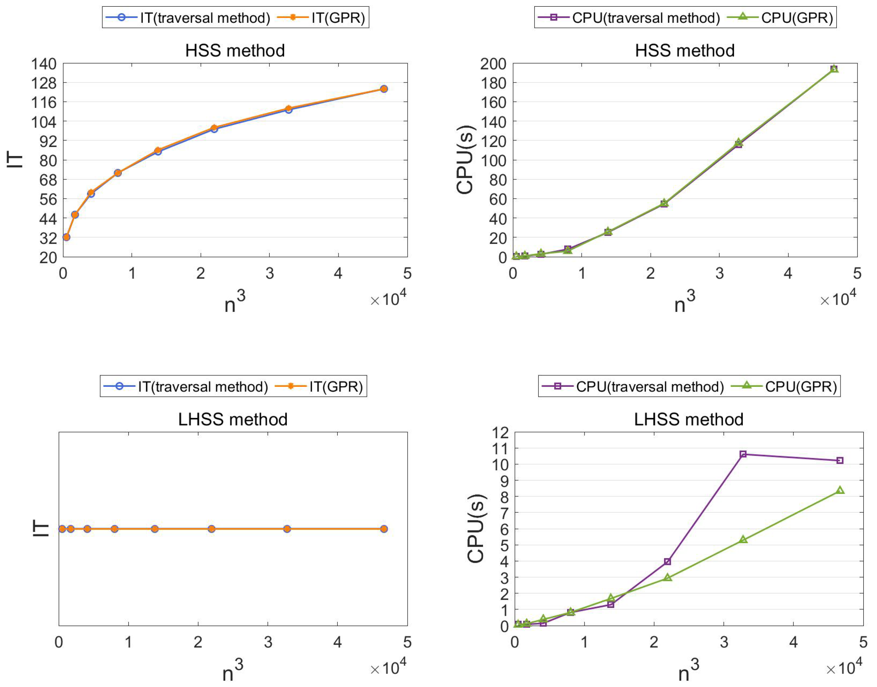
The GPR method vs. the traversal method. We first use the HSS method, the IHSS method, the LHSS method and the ILHSS method to solve the 3D convection-diffusion equation and the splitting parameters are selected using the traversal method and the GPR method, respectively. Table 1, Table 2, Table 3 and Table 4 and Figure 1 show the numerical results.

Table 1.
Results of the HSS method for solving 3D convection-diffusion equation with traversal method and GPR method.

Table 2.
Results of the IHSS method for solving 3D convection-diffusion equation with traversal method and GPR method.

Table 3.
Results of the LHSS method for solving 3D convection-diffusion equation with traversal method and GPR method.

Table 4.
Results of the ILHSS method for solving 3D convection-diffusion equation with traversal method and GPR method.
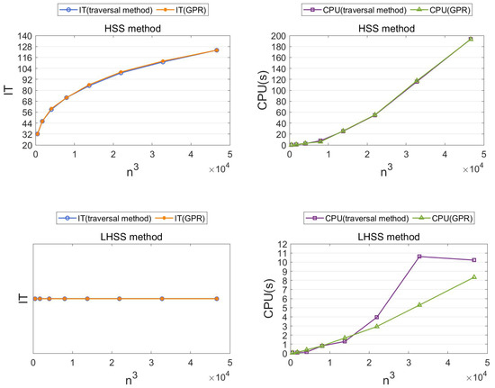
Figure 1.
The IT and CPU of the HSS method and the LHSS method to solve the 3D convection-diffusion equation with splitting parameters selected by the traversal method and the GPR method, respectively.
From Table 1, Table 2, Table 3 and Table 4 and Figure 1, we know that the GPR method can predict almost the same parameters as the traversal method does. It uses a training set from a set of small-scale systems and its training time is much less than the traversal time of the traversal method. Thus, the GPR method requires less calculation than the traversal method.
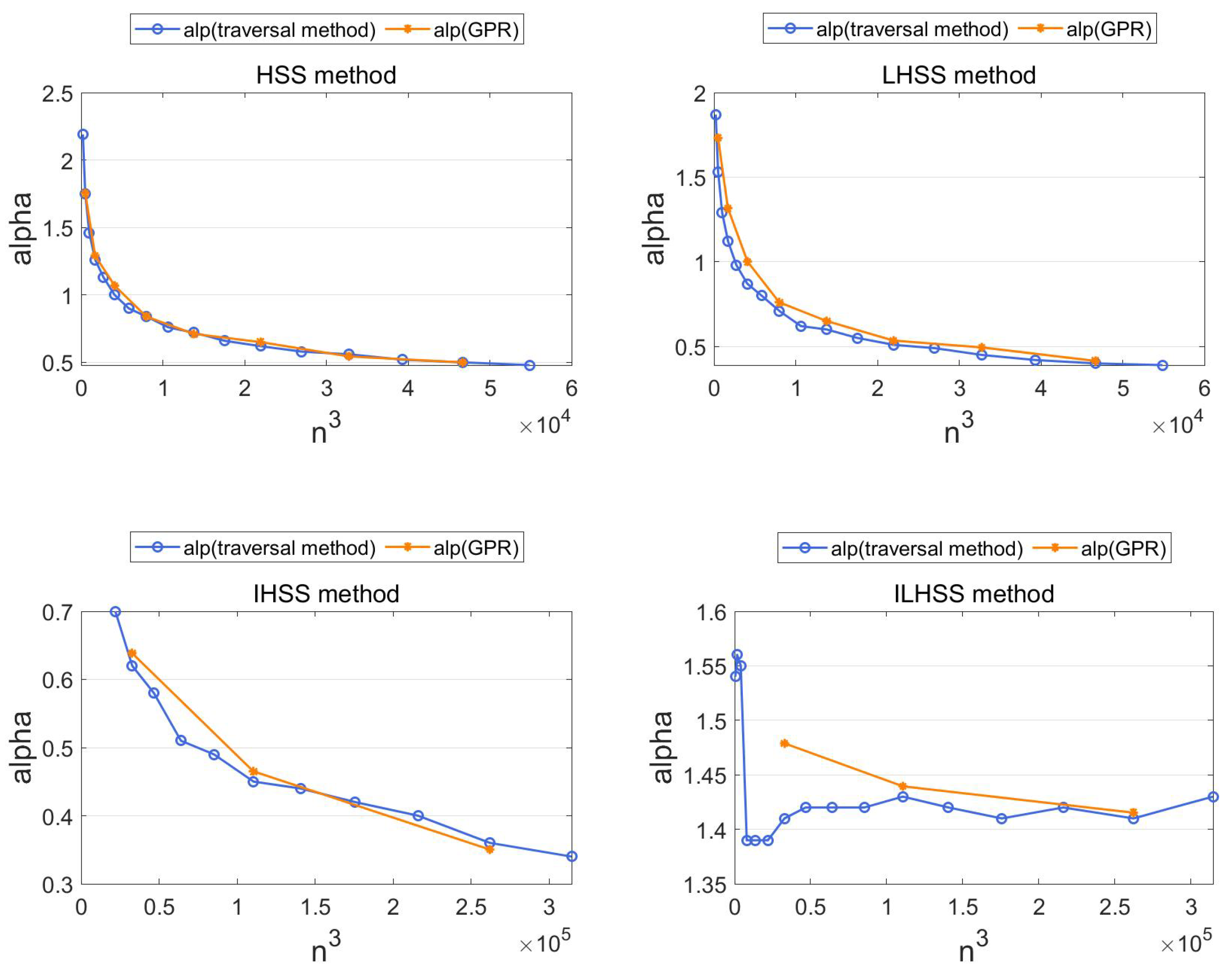
From Figure 2, we can have a visual representation of what the mapping we want to fit looks like.
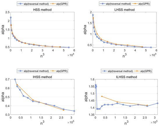
Figure 2.
The splitting parameters of the HSS method, the LHSS method, the IHSS method and the ILHSS method to solve the 3D convection-diffusion equation with splitting parameters selected by the traversal method and the GPR method, respectively.
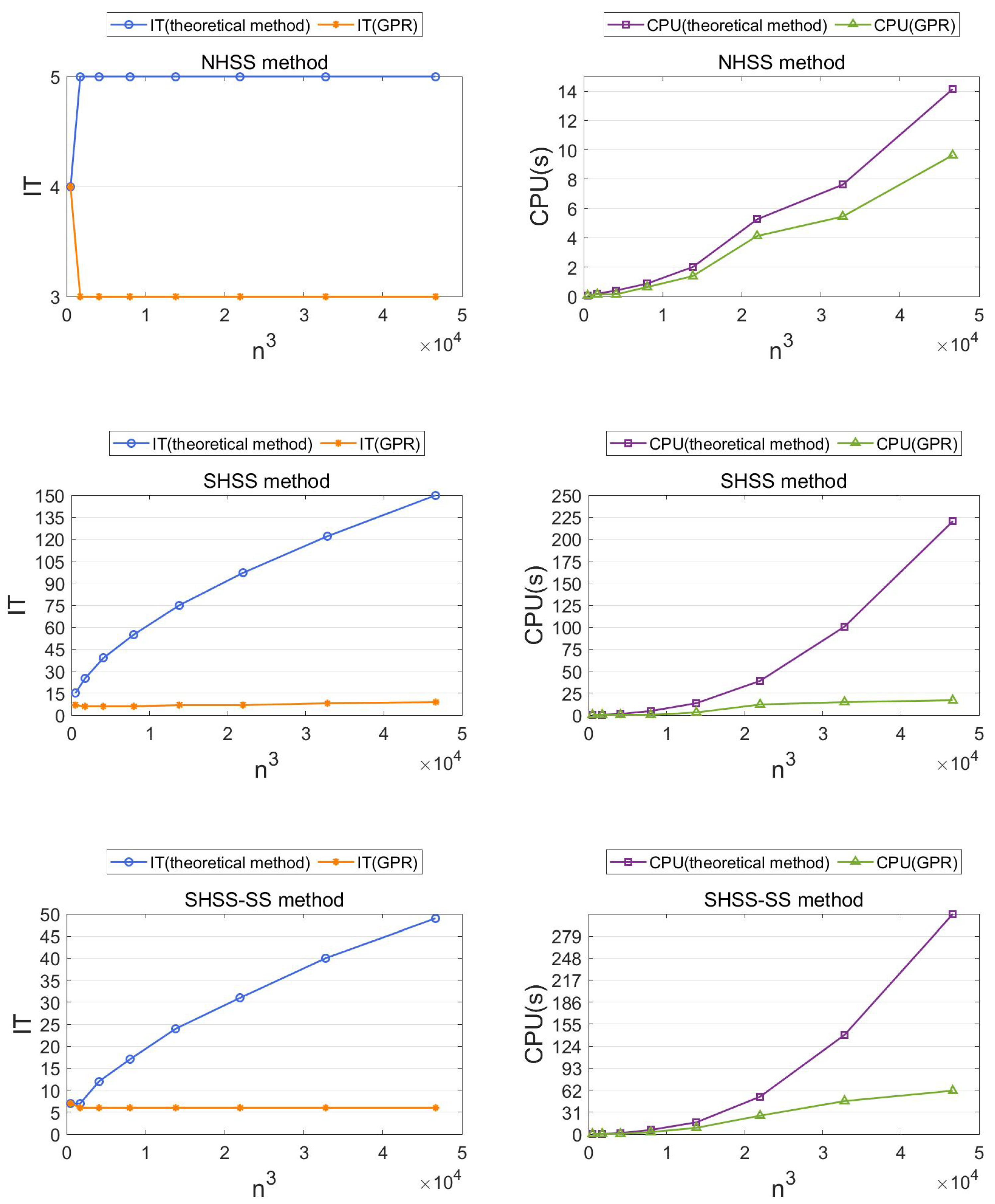
The GPR method vs. the theoretical method. We use the HSS method, the NHSS, the LHSS method, the SHSS method and the SHSS-SS method to solve the 3D convection-diffusion equation, and the splitting parameters are selected using the theoretical method (given in Theorems 3, 5, 7, 9 and 11) and the GPR method, respectively. Table 5, Table 6, Table 7, Table 8 and Table 9 and Figure 3 and Figure 4 show the numerical results.

Table 5.
Results of the HSS method for solving 3D convection-diffusion equation with theoretical method and GPR method.

Table 6.
Results of the LHSS method for solving 3D convection-diffusion equation with theoretical method and GPR method.

Table 7.
Results of the NHSS method for solving 3D convection-diffusion equation with theoretical method and GPR method.

Table 8.
Results of the SHSS method for solving 3D convection-diffusion equation with theoretical method and GPR method.

Table 9.
Results of the SHSS-SS method for solving 3D convection-diffusion equation with theoretical method and GPR method.
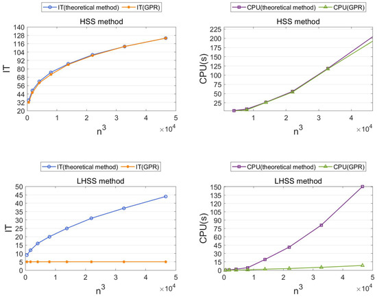
Figure 3.
The IT and CPU of the HSS method and the LHSS method to solve the 3D convection-diffusion equation with splitting parameters selected by the theoretical method and the GPR method, respectively.
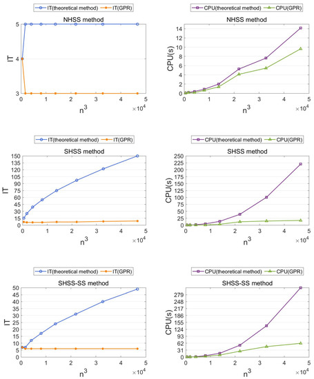
Figure 4.
The IT and CPU of the NHSS method, the SHSS method and the SHSS-SS method to solve the 3D convection-diffusion equation with splitting parameters selected by the theoretical method and the GPR method, respectively.
From Table 5, Table 6, Table 7, Table 8 and Table 9 and Figure 3 and Figure 4, we know that the GPR method can predict better optimal parameters than the theoretical method. Unlike the theoretical method available case-by-case, the GPR method is suitable for the five iterative methods, which means that the GPR method is highly universal.
Example 2.
Consider the following complex symmetric linear systems.
where K is the five-point centered difference matrix approximating the negative Laplacian operator with homogeneous Dirichlet boundary conditions, on a uniform mesh in the unit square with mesh-size . and , with . In addition, the right-hand side vector b with its jth entry is given by
Let and normalize coefficient matrix and right-hand side by multiplying both by . Refer to [53] for more details.
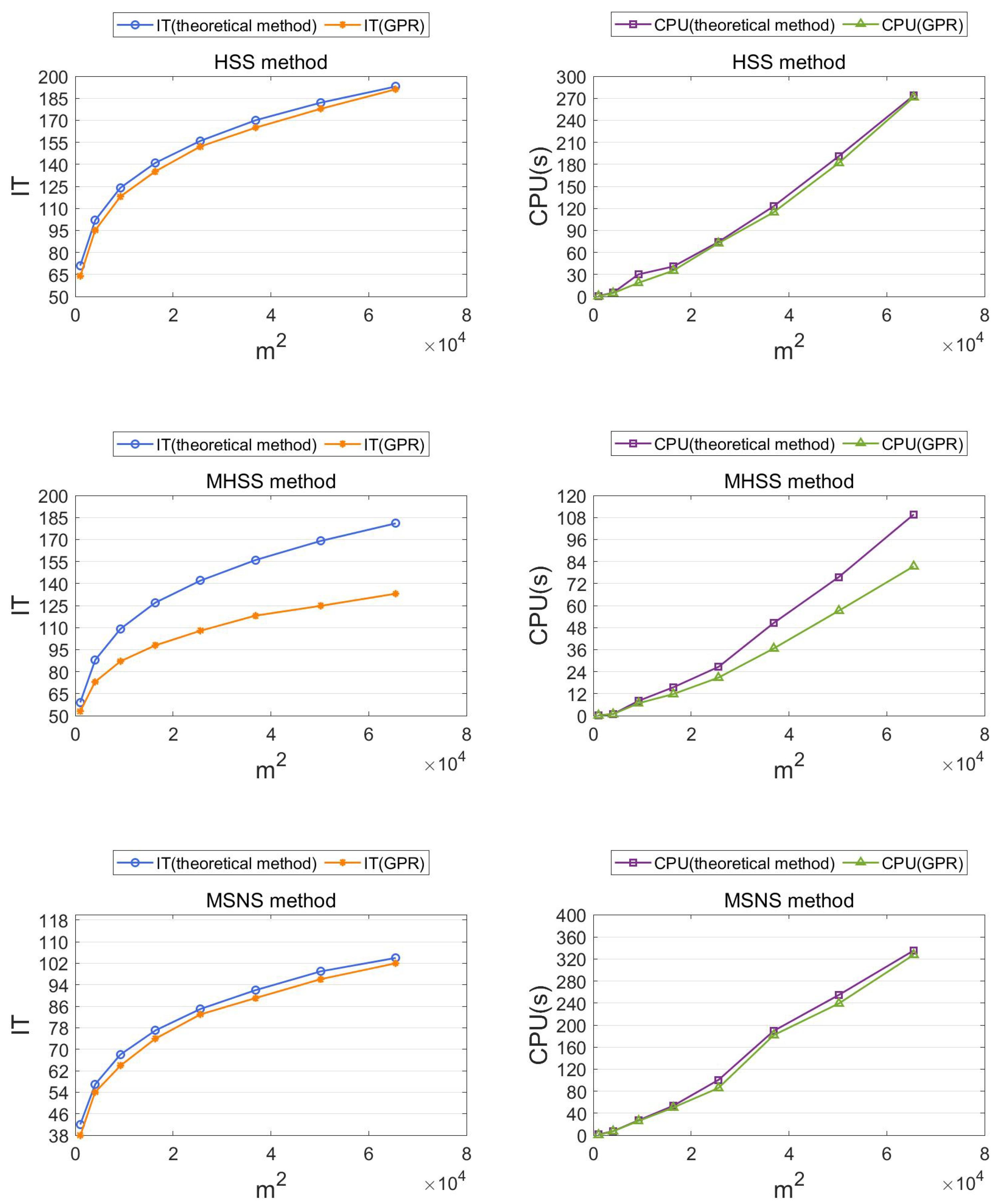
In this experiment, we apply the GPR method to compare with the traversal method and the theoretical method, respectively. Concretely, first, we use the HSS method and the MHSS method to solve Equation (14), and the splitting parameters are selected using the traversal method and the GPR method, respectively. Then, we use the HSS method, the MHSS method and the MSNS method to solve Equation (14), and the splitting parameters are selected using the theoretical method and the GPR method, respectively. Since the extreme eigenvalues of matrix M and extreme singular value of matrix N cannot be explicitly obtained, we use MATLAB built-in function “eigs(MaxIterations’,500,’Tolerance’,1e-5)” and “svds(MaxIterations’,500,’Tolerance’,1e-5)” to calculate them.
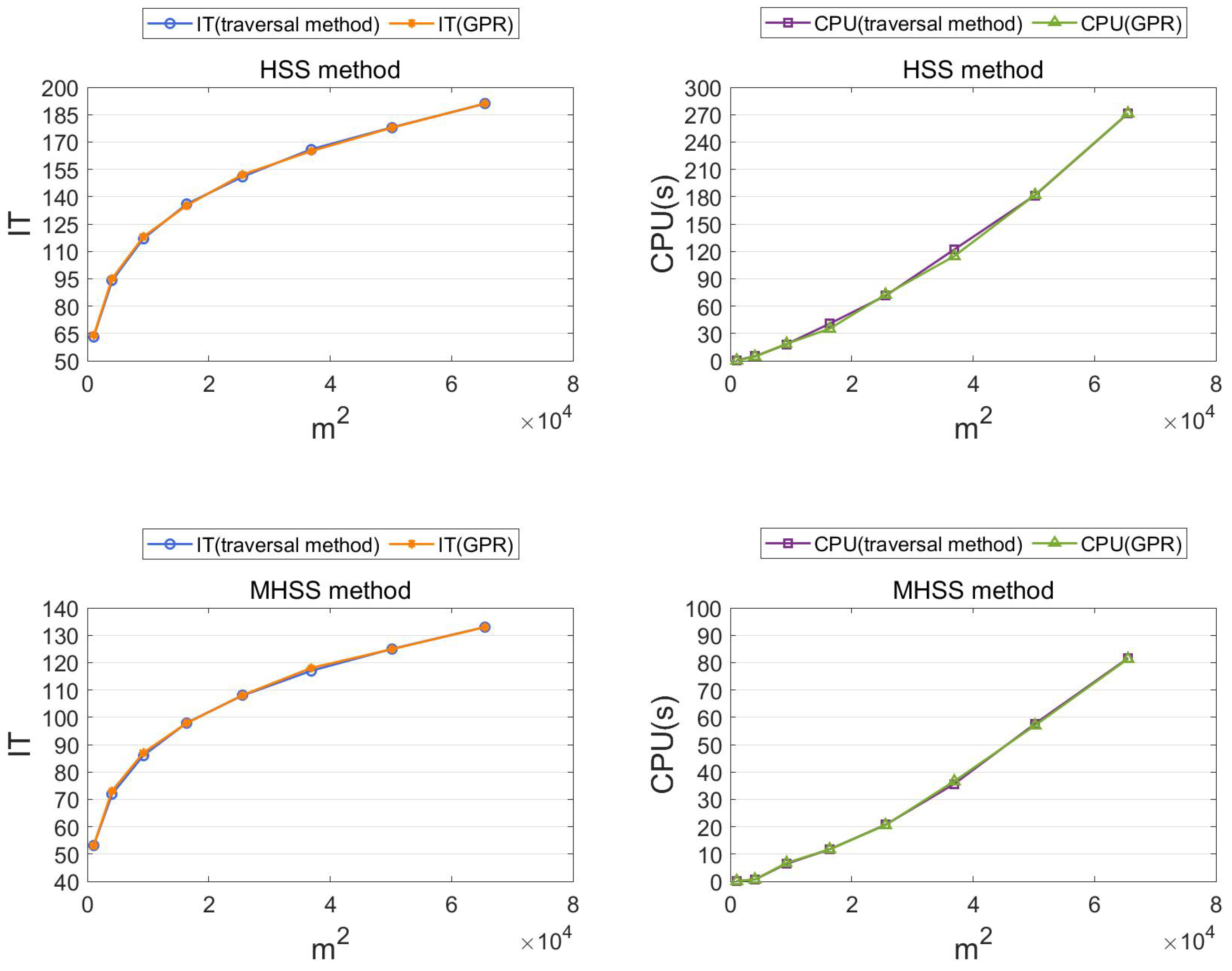
The GPR method vs. the traversal method. We first use the HSS method and the MHSS method to solve Equation (14) and the splitting parameters are selected using the traversal method and the GPR method, respectively. Table 10 and Table 11 and Figure 5 show the numerical results.

Table 10.
Results of the HSS method for solving Equation (14) with traversal method and GPR method.

Table 11.
Results of the MHSS method for solving Equation (14) with traversal method and GPR method.
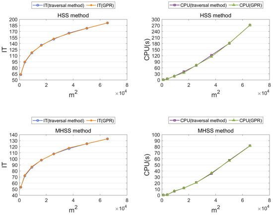
Figure 5.
The IT and CPU of the HSS method and the MHSS method to solve Equation (14) with splitting parameters selected by the traversal method and the GPR method, respectively.
From Table 10 and Table 11 and Figure 5, we know that the GPR method can predict almost the same parameters as the traversal method does. It uses a training set obtained by using the traversal method for small-scale systems and its training time is much less than the traversal time of the traversal method. Thus, the GPR method requires less calculation than the traversal method.
The GPR method vs. the theoretical method. We use the HSS method, the MHSS method and the MSNS method to solve Equation (14), and the splitting parameters are selected using the theoretical method (given in Theorem 3, 13 and 14) and the GPR method, respectively. Table 12, Table 13 and Table 14 and Figure 6 show the numerical results.

Table 12.
Results of the HSS method for solving Equation (14) with theoretical method and GPR method.

Table 13.
Results of the MHSS method for solving Equation (14) with theoretical method and GPR method.

Table 14.
Results of the MSNS method for solving Equation (14) with theoretical method and GPR method.
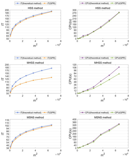
Figure 6.
The IT and CPU of the HSS method, the MHSS method and the MSNS method to solve Equation (14) with splitting parameters selected by the theoretical method and the GPR method, respectively.
From Table 12, Table 13 and Table 14 and Figure 6, we know that the GPR method can predict better optimal parameters than the theoretical method. Unlike the theoretical method only available case-by-case, the GPR method is suitable for the three iterative methods, which means that the GPR method is highly universal.
5. Conclusions
In this paper, we use the Bayesian inference-based Gaussian process regression (GPR) method to predict the relatively optimal parameters of some matrix-splitting iteration methods and provide extensive numerical experiments to compare the prediction performance of the GPR method with other methods. The GPR method learns a mapping between the dimension of linear systems and relatively optimal splitting parameters using a small training data set. Numerical results show that the GPR method requires less calculation than the traversal method. It is more universal and can predict more optimal parameters than the theoretical methods.
There is still lots of work to study the proposed methods. For example, the first one is to apply the GPR method to some iteration methods with multi-parameters or some non HSS-type iteration methods. The second one is to measure the predictive performance of the GPR method when the true optimal parameters to predict are unknown. The third one is to choose other mean functions and covariance functions to improve the predictive performance of the GPR method.
Author Contributions
K.J.—methodology, review and editing; J.S.—software, visualization, data curation; J.Z.—methodology, review and editing. All authors have read and agreed to the published version of the manuscript.
Funding
The work is supported in part by the National Natural Science Foundation of China (12171412, 11771370), Natural Science Foundation for Distinguished Young Scholars of Hunan Province (2021JJ10037), Hunan Youth Science and Technology Innovation Talents Project (2021RC3110), and the Key Project of Education Department of Hunan Province (19A500, 21A0116).
Institutional Review Board Statement
Not applicable.
Informed Consent Statement
Not applicable.
Data Availability Statement
Not applicable.
Conflicts of Interest
The authors declare no conflict of interest.
References
- Young, D. Iterative methods for solving partial difference equations of elliptic type. Trans. Am. Math. Soc. 1954, 76, 92–111. [Google Scholar] [CrossRef]
- Young, D.M. Convergence properties of the symmetric and unsymmetric successive overrelaxation methods and related methods. Math. Comput. 1970, 24, 793–807. [Google Scholar] [CrossRef]
- Hadjidimos, A. Accelerated overrelaxation method. Math. Comput. 1978, 32, 149–157. [Google Scholar] [CrossRef]
- Hadjidimos, A.; Yeyios, A. Symmetric accelerated overrelaxation (SAOR) method. Math. Comput. Simul. 1982, 24, 72–76. [Google Scholar] [CrossRef]
- Darvishi, M.T.; Hessari, P. Symmetric SOR method for augmented systems. Appl. Math. Comput. 2006, 183, 409–415. [Google Scholar] [CrossRef]
- Darvishi, M.T.; Hessari, P. A modified symmetric successive overrelaxation method for augmented systems. Comput. Math. Appl. 2011, 61, 3128–3135. [Google Scholar] [CrossRef]
- Allahviranloo, T. Successive over relaxation iterative method for fuzzy system of linear equations. Appl. Math. Comput. 2005, 162, 189–196. [Google Scholar] [CrossRef]
- Darvishi, M.T.; Hessari, P. On convergence of the generalized AOR method for linear systems with diagonally dominant coefficient matrices. Appl. Math. Comput. 2006, 176, 128–133. [Google Scholar] [CrossRef]
- Bai, Z.Z.; Golub, G.H.; Ng, M.K. Hermitian and skew-Hermitian splitting methods for non-Hermitian positive definite linear systems. SIAM J. Matrix Anal. Appl. 2003, 24, 603–626. [Google Scholar] [CrossRef]
- Bai, Z.Z.; Golub, G.H.; Pan, J.Y. Preconditioned Hermitian and skew-Hermitian splitting methods for non-Hermitian positive semidefinite linear systems. Numer. Math. 2004, 98, 1–32. [Google Scholar] [CrossRef]
- Benzi, M. A generalization of the Hermitian and skew-Hermitian splitting iteration. SIAM J. Matrix Anal. Appl. 2009, 31, 360–374. [Google Scholar] [CrossRef]
- Li, L.; Huang, T.Z.; Liu, X.P. Modified Hermitian and skew-Hermitian splitting methods for non-Hermitian positive-definite linear systems. Numer. Linear Algebra Appl. 2007, 14, 217–235. [Google Scholar] [CrossRef]
- Yang, A.L.; An, J.; Wu, Y.J. A generalized preconditioned HSS method for non-Hermitian positive definite linear systems. Appl. Math. Comput. 2010, 216, 1715–1722. [Google Scholar] [CrossRef]
- Li, L.; Huang, T.Z.; Liu, X.P. Asymmetric Hermitian and skew-Hermitian splitting methods for positive definite linear systems. Comput. Math. Appl. 2007, 54, 147–159. [Google Scholar] [CrossRef]
- Noormohammadi Pour, H.; Sadeghi Goughery, H. New Hermitian and skew-Hermitian splitting methods for non-Hermitian positive-definite linear systems. Numer. Algorithms 2015, 69, 207–225. [Google Scholar] [CrossRef]
- Yang, A.L.; Cao, Y.; Wu, Y.J. Minimum residual Hermitian and skew-Hermitian splitting iteration method for non-Hermitian positive definite linear systems. BIT Numer. Math. 2019, 59, 299–319. [Google Scholar] [CrossRef]
- Li, C.X.; Wu, S.L. A single-step HSS method for non-Hermitian positive definite linear systems. Appl. Math. Lett. 2015, 44, 26–29. [Google Scholar] [CrossRef]
- Li, C.X.; Wu, S.L. A SHSS–SS iteration method for non-Hermitian positive definite linear systems. Results Appl. Math. 2022, 13, 100225. [Google Scholar] [CrossRef]
- Jiang, M.Q.; Cao, Y. On local Hermitian and skew-Hermitian splitting iteration methods for generalized saddle point problems. J. Comput. Appl. Math. 2009, 231, 973–982. [Google Scholar] [CrossRef]
- Benzi, M.; Gander, M.J.; Golub, G.H. Optimization of the Hermitian and skew-Hermitian splitting iteration for saddle-point problems. BIT Numer. Math. 2003, 43, 881–900. [Google Scholar] [CrossRef]
- Krukier, L.A.; Krukier, B.L.; Ren, Z.R. Generalized skew-Hermitian triangular splitting iteration methods for saddle-point linear systems. Numer. Linear Algebra Appl. 2014, 21, 152–170. [Google Scholar] [CrossRef]
- Bai, Z.Z.; Benzi, M. Regularized HSS iteration methods for saddle-point linear systems. BIT Numer. Math. 2017, 57, 287–311. [Google Scholar] [CrossRef]
- Yang, A.L.; Wu, Y.J. The Uzawa–HSS method for saddle-point problems. Appl. Math. Lett. 2014, 38, 38–42. [Google Scholar] [CrossRef]
- Li, X.; Yang, A.L.; Wu, Y.J. Parameterized preconditioned Hermitian and skew-Hermitian splitting iteration method for saddle-point problems. Int. J. Comput. Math. 2014, 91, 1224–1238. [Google Scholar] [CrossRef]
- Wang, X.; Li, Y.; Dai, L. On Hermitian and skew-Hermitian splitting iteration methods for the linear matrix equation AXB = C. Comput. Math. Appl. 2013, 65, 657–664. [Google Scholar] [CrossRef]
- Bai, Z.Z. On Hermitian and skew-Hermitian splitting iteration methods for continuous Sylvester equations. J. Comput. Math. 2011, 29, 185–198. [Google Scholar] [CrossRef]
- Wang, X.; Li, W.W.; Mao, L.Z. On positive-definite and skew-Hermitian splitting iteration methods for continuous Sylvester equation AX + XB = C. Comput. Math. Appl. 2013, 66, 2352–2361. [Google Scholar] [CrossRef]
- Zhou, R.; Wang, X.; Tang, X.B. A generalization of the Hermitian and skew-Hermitian splitting iteration method for solving Sylvester equations. Appl. Math. Comput. 2015, 271, 609–617. [Google Scholar] [CrossRef]
- Zhou, R.; Wang, X.; Tang, X.B. Preconditioned positive-definite and skew-Hermitian splitting iteration methods for continuous Sylvester equations AX + XB = C. East Asian J. Appl. Math. 2017, 7, 55–69. [Google Scholar] [CrossRef]
- Dehghan, M.; Shirilord, A. A generalized modified Hermitian and skew-Hermitian splitting (GMHSS) method for solving complex Sylvester matrix equation. Appl. Math. Comput. 2019, 348, 632–651. [Google Scholar] [CrossRef]
- Bahramizadeh, Z.; Nazari, M.; Zak, M.K.; Yarahmadi, Z. Minimal residual Hermitian and skew-Hermitian splitting iteration method for the continuous Sylvester equation. arXiv 2020, arXiv:2012.00310. [Google Scholar]
- Xu, L.; Mingxiang, L. Generalized positive-definite and skew-hermitian splitting iteration method and its sor acceleration for continuous sylvester equations. Math. Numer. Sin. 2021, 43, 354. [Google Scholar]
- Bai, Z.Z.; Benzi, M.; Chen, F. Modified HSS iteration methods for a class of complex symmetric linear systems. Computing 2010, 87, 93–111. [Google Scholar] [CrossRef]
- Li, X.; Yang, A.L.; Wu, Y.J. Lopsided PMHSS iteration method for a class of complex symmetric linear systems. Numer. Algorithms 2014, 66, 555–568. [Google Scholar] [CrossRef]
- Wu, S.L. Several variants of the Hermitian and skew-Hermitian splitting method for a class of complex symmetric linear systems. Numer. Linear Algebra Appl. 2015, 22, 338–356. [Google Scholar] [CrossRef]
- Bai, Z.Z.; Guo, X.P. On Newton-HSS methods for systems of nonlinear equations with positive-definite Jacobian matrices. J. Comput. Math. 2010, 28, 235–260. [Google Scholar]
- Zhu, M.Z. Modified iteration methods based on the Asymmetric HSS for weakly nonlinear systems. J. Comput. Anal. Appl. 2013, 15, 185–195. [Google Scholar]
- Ke, Y.F.; Ma, C.F. A preconditioned nested splitting conjugate gradient iterative method for the large sparse generalized Sylvester equation. Comput. Math. Appl. 2014, 68, 1409–1420. [Google Scholar] [CrossRef]
- Zheng, Q.Q.; Ma, C.F. On normal and skew-Hermitian splitting iteration methods for large sparse continuous Sylvester equations. J. Comput. Appl. Math. 2014, 268, 145–154. [Google Scholar] [CrossRef]
- Carre, B. The determination of the optimum accelerating factor for successive over-relaxation. Comput. J. 1961, 4, 73–78. [Google Scholar] [CrossRef]
- Kulsrud, H.E. A practical technique for the determination of the optimum relaxation factor of the successive over-relaxation method. Commun. ACM 1961, 4, 184–187. [Google Scholar] [CrossRef]
- Bai, Z.Z.; Golub, G.H.; Li, C.K. Optimal parameter in Hermitian and skew-Hermitian splitting method for certain two-by-two block matrices. SIAM J. Sci. Comput. 2006, 28, 583–603. [Google Scholar] [CrossRef]
- Chen, F. On choices of iteration parameter in HSS method. Appl. Math. Comput. 2015, 271, 832–837. [Google Scholar] [CrossRef]
- Huang, Y.M. A practical formula for computing optimal parameters in the HSS iteration methods. J. Comput. Appl. Math. 2014, 255, 142–149. [Google Scholar] [CrossRef]
- Yang, A.L. Scaled norm minimization method for computing the parameters of the HSS and the two-parameter HSS preconditioners. Numer. Linear Algebra Appl. 2018, 25, e2169. [Google Scholar] [CrossRef]
- Huang, N. Variable-parameter HSS methods for non-Hermitian positive definite linear systems. Linear Multilinear Algebra 2021, 1–18. [Google Scholar] [CrossRef]
- Jiang, K.; Su, X.; Zhang, J. A general alternating-direction implicit framework with Gaussian process regression parameter prediction for large sparse linear systems. SIAM J. Sci. Comput. 2022, 44, A1960–A1988. [Google Scholar] [CrossRef]
- Axelsson, O.; Bai, Z.Z.; Qiu, S.X. A class of nested iteration schemes for linear systems with a coefficient matrix with a dominant positive definite symmetric part. Numer. Algorithms 2004, 35, 351–372. [Google Scholar] [CrossRef]
- Von Mises, R. Mathematical Theory of Probability and Statistics; Academic Press: Cambridge, MA, USA, 2014. [Google Scholar]
- Pourbagher, M.; Salkuyeh, D.K. On the solution of a class of complex symmetric linear systems. Appl. Math. Lett. 2018, 76, 14–20. [Google Scholar] [CrossRef]
- Greif, C.; Varah, J. Iterative solution of cyclically reduced systems arising from discretization of the three-dimensional convection-diffusion equation. SIAM J. Sci. Comput. 1998, 19, 1918–1940. [Google Scholar] [CrossRef]
- Greif, C.; Varah, J. Block stationary methods for nonsymmetric cyclically reduced systems arising from three-dimensional elliptic equations. SIAM J. Matrix Anal. Appl. 1999, 20, 1038–1059. [Google Scholar] [CrossRef]
- Axelsson, O.; Kucherov, A. Real valued iterative methods for solving complex symmetric linear systems. Numer. Linear Algebra Appl. 2000, 7, 197–218. [Google Scholar] [CrossRef]
Publisher’s Note: MDPI stays neutral with regard to jurisdictional claims in published maps and institutional affiliations. |
© 2022 by the authors. Licensee MDPI, Basel, Switzerland. This article is an open access article distributed under the terms and conditions of the Creative Commons Attribution (CC BY) license (https://creativecommons.org/licenses/by/4.0/).

