Abstract
Extended Dynamic Mode Decomposition (EDMD) allows an approximation of the Koopman operator to be derived in the form of a truncated (finite dimensional) linear operator in a lifted space of (nonlinear) observable functions. EDMD can operate in a purely data-driven way using either data generated by a numerical simulator of arbitrary complexity or actual experimental data. An important question at this stage is the selection of basis functions to construct the observable functions, which in turn is determinant of the sparsity and efficiency of the approximation. In this study, attention is focused on orthogonal polynomial expansions and an order-reduction procedure called p-q quasi-norm reduction. The objective of this article is to present a Matlab library to automate the computation of the EDMD based on the above-mentioned tools and to illustrate the performance of this library with a few representative examples.
Keywords:
extended dynamic mode decomposition; Koopman operator; orthogonal polynomials; mathematical modeling; dynamic systems MSC:
37-04
1. Introduction
In contrast to traditional modeling approaches, in which it is necessary to formulate a general nonlinear model that depends on a set of parameters to replicate the dynamics of a system under consideration, the EDMD [1] builds upon numerical data (simulation or actual experiments) to provide a finite-dimensional (truncated) linear representation of the system dynamics in a lifted space of nonlinear observable functions, making it akin to a black box modeling paradigm, e.g., transfer functions or autoregressive models [2,3,4]. While the approximation provided by EDMD therefore remains nonlinear in the original state variables, it is linear in a transformed space, which is called the observable space, function space, or vector-valued function of observables (VVFO), among others (for the remainder of this article, we use observables when referring to this space, while the example codes use the VVFO terminology). In other words, The EDMD formulation does not represent the system by a linearized representation of the form (where A is a Jacobian); rather, it describes the evolution of observables through a linear operator U, i.e.,
EDMD is closely related to other decompositions such as Karhunen–Loeve decomposition (KLD) [5], singular value decomposition (SVD) [6], proper orthogonal decomposition (POD) [7], and its direct precursor, dynamic mode decomposition (DMD) [8]. These decompositions all produce linear approximations of the behavior of the system near a fixed point, offering the possibility of using linear system analysis tools. EDMD extends this possibility to a region of the state space which is larger than the neighborhood of the fixed point. Indeed, EDMD describes the nonlinear dynamics while being linear in the function space, and therefore provides more than local information while preserving the linear characteristics of the above-mentioned decompositions (KLD, SVD, POD, DMD). As such, it is sometimes called a linearization in the large.
Koopman mode decomposition (KMD) [9,10,11] emerges from the linearity of decompositions that use their spectrum (eigenvalues and eigenvectors) to obtain an approximation of the Koopman operator [12]. From an approximation of the Koopman operator, it is possible to analyze nonlinear systems in terms of their stability and regions of attraction [9,13,14,15]. Additionally, EDMD (or the approximate Koopman operator) can be used in the context of optimal control and model predictive control [16,17,18,19]. These developments show the importance of having accurate EDMD approximations for analysis and control.
There are several variants of the EDMD algorithm, which use norm-based expansions, radial-basis functions, kernel-based representations [20], orthogonal polynomials, and their variations [21,22]. These representations provide tools for analyzing nonlinear systems via spectral decomposition, and represent the fundamentals for developing synthesis algorithms such as EDMD for control [23].
In this paper, attention is focused on the use of orthogonal polynomials for the expression of the observable functions and an order reduction method based on p-q quasi norm [24,25]. Several application examples are described together with Matlab codes which constitute a practical library for users interested in applying EDMD to engineering and scientific problems.
The library provides several Matlab functions to compute a pq-EDMD approximation of a dynamical system based on one of three possible algorithms. The first algorithm is the original least squares solution, which is suitable for data with a high signal-to-noise ratio. For data with higher levels of noise, a maximum likelihood approximation is proposed, which is valid for unimodal Gaussian distributions (i.e., Gaussian noise for a system with a unique stable equilibrium point). Finally, a solution based on regularized least squares is provided, which promotes sparsity in the regression matrix.
2. Extended Dynamic Mode Decomposition
This section starts with an introduction to the traditional EDMD formulation to identify nonlinear models of dynamical systems. The procedure is exemplified by the Duffing equation, a benchmark problem in the literature for testing the reliability of the algorithm.
The core idea of the EDMD algorithm is to transform a nonlinear system into an augmented linear system. The first proponent of this idea was Takata [26], who describes the method as a formal linearization. Much later, the method emerged in its current form after the development of the dynamic mode decomposition algorithm [8] and its several extensions. In the following, the original EDMD algorithm [1] is first presented, followed by pq-EDMD, which makes use of orthogonal polynomials and order reduction based on p-q quasi-norm. This later version is particularly interesting as it yields increased numerical accuracy and systematic application.
2.1. The Basic EDMD Formulation
Consider as an example the unforced Duffing oscillator, which is a nonlinear spring that has different behaviors depending on the parameterization. The set of differential equations that govern this system is
where state is the displacement, state is the velocity, is the stiffness of the spring, which is related to the linear force of the spring according to Hooke’s law, is the amount of damping in the system, and is the proportion of nonlinearity present in the stiffness of the spring.
Figure 1 shows the phase plane of the system for three different sets of parameters and six random initial conditions (i.e., six initial conditions are generated randomly within the range starting from a known seed rng(1)). This choice of initial conditions produces an appropriate set of trajectories for calculating the approximation and testing its accuracy. The system of Equations (2) and (3) is integrated with a Matlab ODE solver, e.g., ode23s, and the results are collected at a constant sample period s for a total of 20 s. The result of this numerical integration is a set of six trajectories of two state variables with 201 points per variable. Each of these trajectories is an element of a structure array in Matlab with the fields “Time” and “SV”. The choice of a structure array instead of a tensor comes from the possibility of having trajectories of different lengths, e.g., experimental data of different lengths, a feature that becomes important in systems where having redundant data near the asymptotically stable attractors has a negative impact on the approximation.

Figure 1.
Orbits of the Duffing equation for different parameterizations. (Left): undamped, (Center): hard spring, (Right): soft spring, (Top row): phase plane, (Bottom): states versus time of two trajectories.
As the EDMD is a data-driven algorithm, certain trajectories serve as a training set while others serve as a testing set. The amount of data necessary to obtain an accurate approximation depends on the system under consideration as well as its information content (large data sets can bear little information content if experiments are not properly designed). The EDMD algorithm captures the dynamic of the system on the portion of the state space covered by the trajectories in the training set. Therefore, designing experiments that maximize the coverage of the state space can reduce the amount of data while having a positive effect on accuracy.
Each trajectory of the training set is in discrete-time, i.e., , where are the states of the system, is the non-negative discrete time, and is an unknown nonlinear mapping that provides the evolution of the discretetime trajectories. To construct the database, the training trajectories are organized in so-called snapshot pairs , where . The snapshots function presented in Listing 1 handles the available trajectories, dividing them into training and testing sets of the appropriate type; the training set consists of matrices containing the x and y data, while the testing set is a cell array containing one orbit per index of the cell. The choice of cell arrays instead of a tensor is to offer the possibility of testing trajectories of different lengths. The tr_ts argument is a Matlab structure containing the indexes of the original set of orbits, which serve as the training and testing sets. The fields of this structure must be tr_index and ts_index, respectively. In addition, there is a normalization flag to use when necessary, e.g., when the order of magnitude of different states is dissimilar.
| Listing1. Function snapshots used to create the data pairs for training and testing. |
 |
Notice that the generation of the snapshots avoids the last element in each trajectory, SV(1:end-2) for x and SV(2:end-1) for y. As stated before, avoiding redundant data at the asymptotically stable attractors improves the performance of the algorithm. In Matlab, stopping the simulation early, e.g., as convergence towards the attractor has been achieved, causes the last output interval . This small difference can increase the error in the construction of the approximation. Conversely, if the numerical integration of the system is not stopped near the steady state, it is not necessary to eliminate the last element in the trajectories.
The next step in the development of the EDMD is the definition of the observable space as a set of functions for , which represent a transformation from the state space into an arbitrary function space. This transformation of the state is equivalent to a change of variables , where . In the Matlab library, the observables are described by orthogonal polynomials, where each element of the set of observables is the tensor product of n univariate polynomials up to order . For example, in the Duffing oscillator, a set of observables with and a Hermite basis of orthogonal polynomials is provided by
Note that the first entry is the product of a zero-order polynomial in both of the state variables; the orders of the polynomial basis in the two state variables can be summarized by
making the generation of observables a problem of accurately handling indexes. Notice that the full basis of indexes (5) is equivalent to counting numbers on a basis with n significant figures. From such a set of indexes, a method to generate a set of observables with a Hermite base is proposed in Listing 2.
| Listing2. Generation of a set of observables with a Hermite basis. |
 |
The function f can evaluate the complete set of training trajectories at once with the omission of the first observable that corresponds to the intercept or constant value (the consideration of this observable would require another programming strategy involving loops, resulting in higher computational time and memory allocation). Notice the versatility of using orthogonal polynomials, as the whole realm of available orthogonal polynomials in Matlab is a valid choice, e.g., Laguerre, Legendre, Jacobi, etc. Note that the code snippet defines the function of observables as a row vector, instead of the column vector notation in the theoretical descriptions.
After the observables have been defined, their time evolution can be computed according to
where is the matrix that provides the linear evolution of the observables and is the error in the approximation. One of the main advantages of the EDMD algorithm resides in the fact that the system description is linear in the function space. The solution to (6) is the matrix U that minimizes the residual term , which can be expressed as a least-squares criterion:
where N is the total number of samples in the training set. The ordinary least-squares (OLS) solution is provided by
where the notation replaces the inverse of the design matrix G, as even when using a basis formed by the products of orthogonal polynomials, the design matrix can be close to ill-conditioned (i.e., close to singular). This notation, particularly in Matlab, specifies that a more robust algorithm compared to the inverse or pseudo-inverse is necessary to obtain the approximation.
Setting the observables as products of univariate orthogonal polynomials is an improvement, as it generally avoids the need to use a pseudo-inverse approach. Even though the sequence of polynomials in the set of observables is no longer orthogonal, it is less likely to have co-linear columns in the design matrix, improving the numerical stability of the solution. With the training set and the observables, the method for calculating the regression matrix U is shown in Listing 3. Notice that this code defines and uses all the arrays as their transpose. This change is related to the approximation of the Koopman operator, where it is necessary to calculate the right and left eigenvectors of U. The eigenfunctions of the Koopman operator are determined from the left eigenvectors of the spectral decomposition. In Matlab, the left eigenvectors result from additional algebraic manipulations of the right eigenvectors and the diagonal matrix of eigenvalues, thereby decreasing the numerical precision of the eigenfunctions. This problem is alleviated by computing and its spectral decomposition so that the left eigenvectors are immediately available. In general, if U is a normal matrix (diagonalizable), the additional steps involve the inverse of the right eigenvectors to obtain the left eigenvectors and the calculation of this inverse, considering again that the problem is close to being ill-conditioned, which reduces the accuracy of the eigenfunctions.
| Listing3. Computation of the approximate Koopman operator for an OLS problem. |
 |
Numerical Results with EDMD
Here, the EDMD algorithm is tested with the second case scenario for the Duffing oscillator with hard damping. The EDMD algorithm can capture the dynamics of the portion of the state space covered by the training set, which is therefore selected as the outermost trajectory in Figure 2. The five remaining trajectories are used for testing. Table 1 provides the parameters of the original EDMD algorithm.
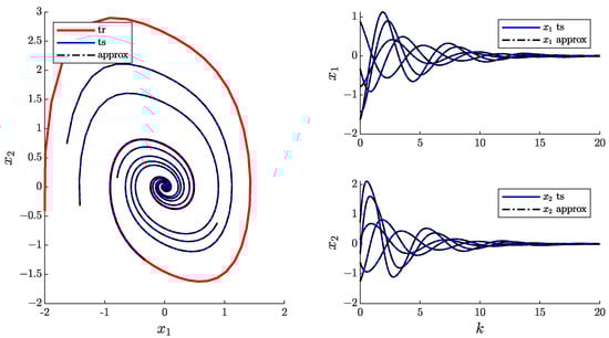
Figure 2.
EDMD approximation of the hard damping Duffing oscillator.

Table 1.
Approximation parameters for the hard spring Duffing oscillator.
In Figure 2, the graph on the left displays the phase plane of the system and shows the training trajectory and testing trajectories along with their approximation by the EDMD algorithm with the Laguerre polynomial basis. EDMD achieves a good approximation while using only a small amount of data. However, notice that the discrete-time approximation of a system of order 2 is of dimension twenty-five. In view of this dimensionality explosion with regard to the original dimension of the state and the complexity of the system, it is necessary to introduce reduction techniques that decrease the necessary number of observables to increase the accuracy of the algorithm [24].
2.2. pqEDMD Algorithm
The extension of the EDMD algorithm is a result of speculation on the good performance of the original algorithm when coupled with a set of observables based on products of univariate-orthogonal polynomials. The idea is to introduce a reduction method, based on p-q quasi-norms, first introduced by Konakli and Sudret [27] for fault detection in polynomial chaos problems. The reduction proceeds in the following way: if the q-quasi-norm of the indexes that provide the order of the univariate-orthogonal polynomials is less than the maximum order p of a particular observer, then this observer is eliminated from the set. To implement this procedure, the orders of an observer are defined as , and the q-quasi norm of these orders as
where and Equation (11) represent a norm only when q is an integer. When p is redefined as the maximum order of a particular multivariate polynomial instead of the maximum order of the univariate elements, the sets of polynomial orders that remain in the basis are those that satisfy
The code snippet used to generate a set of observables based on Laguerre polynomials with a maximum multivariate order and a q-quasi-norm is provided in Listing 4.
The reduction of the basis is not only dimensional, as the p-q quasi-norm reduction reduces the maximum order of the observables as well. As a rule of thumb (considering various application examples), the higher-order observables usually have a negative contribution to the accuracy of the solution.
| Listing4. Generation of a p-q-reduced set of observables with a Laguerre basis. |
 |
Numerical Results with the pqEDMD
The algorithm is now applied to the Duffing oscillator with soft damping. The pqEDMD algorithm can capture the dynamics of the two attractors provided that the training set has at least one trajectory that converges to each of them. Additionally, as is the case for the hard damping, each of these trajectories should be the outermost (see Figure 3). Table 2 lists the parameters of the pqEDMD algorithm.

Figure 3.
pqEDMD approximation for the soft damping Duffing oscillator.
Table 2.
Approximation parameters for the soft spring Duffing oscillator.
Even though the full basis achieves a low approximation error of , the reduction of the observables order reduces the empirical error by two orders of magnitude. Comparing the dimension of the full basis to the reduced one does not represent a large improvement. However, this result is due to the comparison between the best result after performing a sweep over several p-q values. Imposing lower p-q values on the approximation has the potential to provide smaller sets of observables while sacrificing accuracy.
Next, the first case scenario is considered; here, the damping parameter is zero and the system oscillates around the fixed point at the origin. The pqEDMD algorithm can capture the dynamics of the system if the innermost and outermost limit cycles compose the training set; otherwise, the algorithm cannot capture the dynamics. Table 3 shows a summary of the simulations along with the results; it is apparent that even though the empirical error is higher than in the other two case scenarios, the approximation is accurate (see Figure 4).
Table 3.
Approximation parameters for the undamped Duffing oscillator.
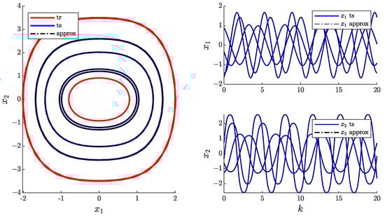
Figure 4.
pqEDMD approximation for the undamped Duffing oscillator.
The sweep over different p-q values provides a reduced basis with lower error than with the full basis.
Even though p-q quasi-norm reduction produces more accurate and tractable solutions, having products of orthogonal univariate polynomials does not necessarily produce an orthogonal basis. In certain scenarios, the evaluation of the observables produces an ill-conditioned design matrix G. Therefore, the next section proposes a way to eliminate even more observables from the basis, improving the numerical stability of the solution.
2.3. Improving Numerical Stability via QR Decomposition
QR decomposition [28] can be used to improve the numerical stability and reduce the number of observables even further. If we assume that the design matrix in Equation (9) is obtained based on the products of orthogonal polynomials and that there are no co-linear columns, or, in other words, that holds, then it is possible to decompose this matrix into the product
where is orthogonal, i.e., and is upper triangular. Column pivoting methods for QR decomposition rely on exchanging the rows of G such that in every step of the diagonalization of R and the subsequent calculation of the orthogonal columns of Q the procedure starts with a column that is as independent as possible from the columns of G already processed. This method yields a permutation matrix such that
where the permutation of columns makes the absolute value of the diagonal elements in R non-increasing, i.e., . Furthermore, considering that the permutation process selects the most linearly independent column of G in every step of the process, the last columns in the analysis are the ones that are close to being co-linear. Therefore, eliminating the observable related to the last column improves the residual condition number of G. The modified function for the calculation of the regression matrix U is provided in Listing 5.
| Listing5. Computation of the regression matrix based on QR decomposition. |
 |
In addition, the code snippet shows particular aspects of the overall solution. First, an object containing the observables, i.e., the matlabFunction obj.VVFO.Psi, replaces the original matlabFunction f for the evaluation of the snapshots. Second, note that the exclusion of observables avoids the elimination of the first order univariate polynomials in the basis, as they are used to recover the state. Finally, the method checks for the existence of the constant observable or the intercept, as it could be eliminated due to being close to co-linear with another observable, which we obviously do not want to happen.
2.4. Matlab Package
pqEDMD() is the main class of the Matlab package that provides an array of decompositions based on the pqEDMD algorithm pqEDMD_array. The cardinality of the array of solutions may be less than the product of the cardinality of p and q, as certain p-q pairs produce the same set of indices, i.e., the algorithm would compute the same decomposition more than once. In addition, it calculates the empirical error of the approximations based on the test set and returns the best-performing approximation from the array as a separate attribute best_pqEDMD. The code provides the complete set of solutions, as a user may opt to use a compact solution that is not as accurate as the best one for tractability reasons, e.g., an MPC controller, where a smaller basis guarantees feasibility for longer horizons and has a lower computational cost.
The only required input for pqEDMD() is the system argument, where it is necessary to provide a structure array with the Time and SV fields with at least two trajectories in the array, one for training and one for testing. The remaining arguments are optional, e.g., the array of positive-integer values p, the array of positive values q, the structure of training and testing trajectories with the fields tr_index and ts_index, the string specifying the type of polynomial, the array of polynomial parameters (if the polynomial type is either “Jacobi” or “Gegenbauer”), the boolean flag of normalization, and the string indicating the decomposition method. For example, Listing 6 shows a call to the algorithm with a complete set of arguments.
| Listing6. Complete call to the pqEDMD algorithm. |
 |
To provide the different approximations in the main class, pqVVFO() handles the observables for different values of p, q, and the polynomial type. Its output is the matrix of polynomial indexes, a symbolic vector of observable functions, and a matlabFunction Psi to evaluate the observables arithmetically and efficiently; it accepts a matrix of values, avoiding evaluation with loops.
The remaining classes are the implementations of different decompositions based on different algorithms. The ExtendedDecomposition() is the traditional least-squares method described in this article. In addition, there are two additional available decompositions. MaxLikeDecomposition() is used for data with noise, where the maximum likelihood algorithm assumes that the transformation of the states in the function space preserves a unimodal Gaussian distribution of the noise in the state space (this is a work in progress; preliminary results can be found in [29]). These properties of the distribution of noise in the function space are a strong assumption; nonetheless, it is sometimes possible to identify dynamical systems corrupted with noise. The last decomposition leverages the advantages of regularized lasso regression to produce sparse solutions, i.e., RegularizedDecomposition(). Even though the solutions are more tractable, the regularized method sacrifices accuracy.
Figure 5 shows the architecture of the solution with the relationship between classes. The current functionality requires the user to call pqEDMD() with the appropriate inputs and options in order to obtain an array of decompositions. This class handles the creation of the necessary pqVVFO() objects to feed into the required decomposition. It is possible to use and extend the observable class to use in other types of decompositions without the use of the main class. The code is available for download in the Supplementary Materials section of this paper.

Figure 5.
Package architecture.
3. An Additional Application Example
To conclude this article, an additional case study is discussed involving a set of reactions occurring in a continuously stirred tank reactor, described by
where there are two types of substrate, and . The first substrate is the only component in the inflow, and is the only component necessary for the replication of the first species according to the replication rate constant . In addition to the replication of , the product of the first reaction is the second substrate , which in turn is necessary for the replication of the second species according to the replication rate constant . The remaining variable is the combination of the dead species from the two groups, where each group dies according to the reaction rates and , respectively. The ordinary differential equations that describe the dynamics of network (15) according to the polynomial formulation of mass action kinetics [30] and the material exchange with the environment are provided by
where is the in/out-flow (dilution rate) of the system and the values for the reaction rates are . With these rate constants, the system has three asymptotically stable points: the working point, where the two species and coexist, a point where species thrives and species washes out, and a wash-out point, where the concentration of both species vanishes. To construct the database, the strategy is to generate a set of orbits with an even distribution of initial conditions converging to each of the equilibrium points. Certain trajectories converging to each point are used as the training set to produce a linear expanded approximation of the system.
The set of orbits is taken from the numerical integration of the ODE (16) via the ode23s method with an output sampling for an arbitrary number of initial conditions until the full set of orbits has a total of 20 trajectories that converge to each point, resulting in 60 trajectories in total for the execution of the algorithm.
From each of the sets of orbits that converge to the fixed points, are used for the approximation and the remaining for testing the solution. It is important to have a training set with sufficient information about the trajectories of the system, and in a similar way as for the second and third scenarios of the Duffing equation, to select the trajectories that are far away from the equilibrium point. For system (16), the choice of trajectories for the training set are the ten trajectories that at any given time are furthest away from the equilibrium point to which they converge. Figure 6 shows a selection of training and testing trajectories.
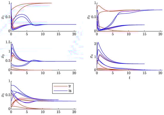
Figure 6.
Training and testing trajectories of the biochemical reaction system.
Assuming that the orbits of the system are in a structure array with the appropriate fields named system and that the training and testing indexes for the approximation have been carefully selected and placed in a structure named tr_ts, the call to the pqEDMD() class that provides an accurate approximation is shown in Listing 7, where the solution is obtained through the default decomposition method (ordinary least squares), the default polynomial type (Legendre), and without normalization.
| Listing7. Class call to approximate the reaction network dynamics. |
 |
Table 4 shows a summary of the simulation parameters used to generate the orbits and to obtain the approximation. The clear advantage of using the reduction method lies in the comparison between the full basis of polynomials, i.e., from 3125 observables for and a system of five state variables to a basis of 51 polynomials for . Although the computation with a full basis is computationally intensive, it leads to a solution that is not satisfactory, as the state matrix is not Hurwitz and the trajectories diverge, leading to a result with an infinite error metric.
Table 4.
Approximation parameters for the reaction network.
Figure 7 depicts the comparison of several testing trajectories with their corresponding approximations. It is clear that certain trajectories converge to a different fixed point than the one they are supposed to. This phenomenon causes the empirical error grow while remaining bounded. The reason for this behavior is the lack of training trajectories near the boundary of the attraction regions of the asymptotically stable equilibrium points. For better performance of the algorithm in terms of the number of orbits necessary for the approximation, and possibly the dimension of the observable basis, an experimental design procedure is required.

Figure 7.
Comparison between the testing and approximation trajectories of the biochemical reaction system.
4. Conclusions
This paper presents a methodology to derive discrete-time approximations of nonlinear dynamical systems via the pqEDMD algorithm and proposes a Matlab library that can hopefully help popularize the use of the method by non-expert users. The discussion of the methodology and codes is illustrated with several case studies related to the Duffing oscillator and by an example involving a biochemical reaction network.
Supplementary Materials
The following supporting information can be downloaded at: https://www.mdpi.com/article/10.3390/math10203859/s1. A Matlab library is readily available in the Supplementary Materials.
Author Contributions
Conceptualization, C.G.-T. and A.V.W.; methodology, C.G.-T. and A.V.W.; software, C.G.-T.; writing—review and editing, C.G.-T. and A.V.W. All authors have read and agreed to the published version of the manuscript.
Funding
This research received no external funding.
Data Availability Statement
Not applicable.
Conflicts of Interest
The authors declare no conflict of interest.
References
- Williams, M.O.; Kevrekidis, I.G.; Rowley, C.W. A Data-Driven Approximation of the Koopman Operator: Extending Dynamic Mode Decomposition. J. Nonlinear Sci. 2015, 25, 1307–1346. [Google Scholar] [CrossRef]
- Ljung, L. System Identification: Theory for the User, 2nd ed.; Prentice Hall: Hoboken, NJ, USA, 1999. [Google Scholar]
- John, L.; Crassidis, J.L.J. Optimal Estimation of Dynamic Systems, 1st ed.; Chapman & Hall/CRC Applied Mathematics & Nonlinear Science; Chapman and Hall/CRC: Boca Raton, FL, USA, 2004. [Google Scholar]
- Penny, W.; Harrison, L. CHAPTER 40—Multivariate autoregressive models. In Statistical Parametric Mapping; Friston, K., Ashburner, J., Kiebel, S., Nichols, T., Penny, W., Eds.; Academic Press: London, UK, 2007; pp. 534–540. [Google Scholar]
- Roger, G.; Ghanem, P.D.S. Stochastic Finite Elements: A Spectral Approach, Revised ed.; Dover Publications: Mineola, NY, USA, 2003. [Google Scholar]
- Stewart, G.W. On the Early History of the Singular Value Decomposition. SIAM Rev. 1993, 35, 551–566. [Google Scholar] [CrossRef]
- Chatterjee, A. An introduction to the proper orthogonal decomposition. Curr. Sci. 2000, 78, 808–817. [Google Scholar]
- Schmid, P.J. Dynamic mode decomposition of numerical and experimental data. J. Fluid Mech. 2010, 656, 5–28. [Google Scholar] [CrossRef]
- Mezić, I. Spectral Properties of Dynamical Systems, Model Reduction and Decompositions. Nonlinear Dyn. 2005, 41, 309–325. [Google Scholar] [CrossRef]
- Mezić, I.; Mezi, I. On applications of the spectral theory of the Koopman operator in dynamical systems and control theory. In Proceedings of the 2015 54th IEEE Conference on Decision and Control (CDC), Osaka, Japan, 16–18 December 2015; pp. 7034–7041. [Google Scholar]
- Mezic, I.; Surana, A. Koopman Mode Decomposition for Periodic/Quasi-periodic Time Dependence—The funding provided by UTRC is greatly appreciated. IFAC-PapersOnLine 2016, 49, 690–697. [Google Scholar] [CrossRef]
- Koopman, B.O. Hamiltonian Systems and Transformation in Hilbert Space. Proc. Natl. Acad. Sci. USA 1931, 17, 315–318. [Google Scholar] [CrossRef]
- Mauroy, A.; Mezić, I. A spectral operator-theoretic framework for global stability. In Proceedings of the 52nd IEEE Conference on Decision and Control, Firenze, Italy, 10–13 December 2013; pp. 5234–5239. [Google Scholar]
- Mauroy, A.; Mezic, I. Global Stability Analysis Using the Eigenfunctions of the Koopman Operator. IEEE Trans. Autom. Control 2016, 61, 3356–3369. [Google Scholar] [CrossRef]
- Garcia-Tenorio, C.; Tellez-Castro, D.; Mojica-Nava, E.; Vande Wouwer, A. Evaluation of the Region of Attractions of Higher Dimensional Hyperbolic Systems using the Extended Dynamic Mode Decomposition. arXiv 2022, arXiv:2209.02028. [Google Scholar]
- Brunton, S.L.; Brunton, B.W.; Proctor, J.L.; Kutz, J.N. Koopman invariant subspaces and finite linear representations of nonlinear dynamical systems for control. PLoS ONE 2016, 11, e0150171. [Google Scholar] [CrossRef]
- Korda, M.; Mezić, I. Linear predictors for nonlinear dynamical systems: Koopman operator meets model predictive control. Automatica 2018, 93, 149–160. [Google Scholar] [CrossRef]
- Tellez-Castro, D.; Garcia-Tenorio, C.; Mojica-Nava, E.; Sofrony, J.; Vande Wouwer, A. Data-Driven Predictive Control of Interconnected Systems Using the Koopman Operator. Actuators 2022, 11, 151. [Google Scholar] [CrossRef]
- Garcia-Tenorio, C.; Vande Wouwer, A. Extended Predictive Control of Interconnected Oscillators. In Proceedings of the 2022 8th International Conference on Control, Decision and Information Technologies (CoDIT), Istanbul, Turkey, 17–20 May 2022; Volume 1, pp. 15–20. [Google Scholar]
- Williams, M.O.; Rowley, C.W.; Kevrekidis, I.G. A kernel-based method for data-driven koopman spectral analysis. J. Comput. Dyn. 2016, 2, 247–265. [Google Scholar] [CrossRef]
- Kaiser, E.; Kutz, J.N.; Brunton, S.L. Sparse identification of nonlinear dynamics for model predictive control in the low-data limit. Proc. R. Soc. A Math. Phys. Eng. Sci. 2018, 474, 20180335. [Google Scholar] [CrossRef] [PubMed]
- Li, Q.; Dietrich, F.; Bollt, E.M.; Kevrekidis, I.G. Extended dynamic mode decomposition with dictionary learning: A data-driven adaptive spectral decomposition of the Koopman operator. Chaos Interdiscip. J. Nonlinear Sci. 2017, 27, 103111. [Google Scholar] [CrossRef]
- Proctor, J.L.; Brunton, S.L.; Kutz, J.N. Dynamic Mode Decomposition with Control. SIAM J. Appl. Dyn. Syst. 2016, 15, 142–161. [Google Scholar] [CrossRef]
- Garcia-Tenorio, C.; Delansnay, G.; Mojica-Nava, E.; Vande Wouwer, A. Trigonometric Embeddings in Polynomial Extended Mode Decomposition—Experimental Application to an Inverted Pendulum. Mathematics 2021, 9, 1119. [Google Scholar] [CrossRef]
- Garcia-Tenorio, C.; Mojica-Nava, E.; Sbarciog, M.; Vande Wouwer, A. Analysis of the ROA of an anaerobic digestion process via data-driven Koopman operator. Nonlinear Eng. 2021, 10, 109–131. [Google Scholar] [CrossRef]
- Takata, H. Transformation of a nonlinear system into an augmented linear system. IEEE Trans. Autom. Control 1979, 24, 736–741. [Google Scholar] [CrossRef]
- Konakli, K.; Sudret, B. Polynomial meta-models with canonical low-rank approximations: Numerical insights and comparison to sparse polynomial chaos expansions. J. Comput. Phys. 2016, 321, 1144–1169. [Google Scholar] [CrossRef]
- Gander, W. Algorithms for the QR decomposition. Res. Rep 1980, 80, 1251–1268. [Google Scholar]
- Garcia-Tenorio, C.; Vande Wouwer, A. Maximum Likelihood pqEDMD Identification. In Proceedings of the 26th International Conference on System Theory, Control and Computing 2022 (ICSTCC), Sinaia, Romania, 19–21 October 2022. [Google Scholar]
- Chellaboina, V.; Bhat, S.P.; Haddad, W.M.; Bernstein, D.S. Modeling and analysis of mass-action kinetics. IEEE Control Syst. Mag. 2009, 29, 60–78. [Google Scholar]


Publisher’s Note: MDPI stays neutral with regard to jurisdictional claims in published maps and institutional affiliations. |
© 2022 by the authors. Licensee MDPI, Basel, Switzerland. This article is an open access article distributed under the terms and conditions of the Creative Commons Attribution (CC BY) license (https://creativecommons.org/licenses/by/4.0/).