Abstract
A class of problems of wave propagation in waveguides consisting of one or several layers that are characterized by linear variation of the squared refractive index along the normal to the interfaces between them is considered in this paper. In various problems arising in practical applications, it is necessary to efficiently solve the dispersion relations for such waveguides in order to compute horizontal wavenumbers for different frequencies. Such relations are transcendental equations written in terms of Airy functions, and their numerical solutions may require significant computational effort. A procedure that allows one to reduce a dispersion relation to an ordinary differential equation written in terms of elementary functions exclusively is proposed. The proposed technique is illustrated on two cases of waveguides with both compact and non-compact cross-sections. The developed reduction method can be used in applications such as geoacoustic inversion.
Keywords:
underwater acoustics; diffraction; dispersion relation; special functions; nonlinear ordinary differential equation MSC:
35L05; 76Q05
1. Introduction
Problems the involving propagation of guided waves are ubiquitous in many fields of physics. Important particular areas of their applications include but are not restricted to optics, physical oceanography, acoustics, geophysics, and radio wave theory. Solutions of both direct and inverse problems for guided waves are often best accomplished in the framework of mode theory. In order to make use of the latter approach, one has to be able to efficiently solve dispersion relations. This is especially important in broadband simulations where such relations must be solved for many frequencies. Apart from purely numerical approaches, it is always useful to have some techniques for the semi-analytical representation of dispersion relation solutions. A very important case when such a semi-analytical representation exists is the layered medium where the refractive index squared is a piecewise linear function of the coordinate transverse to the propagation axis [1,2,3,4,5,6]. Such a model can, in principle, be efficiently used in many cases when the media parameters are specified on a relatively coarse discrete grid. This is especially important for such applications as radio waves [6], underwater acoustics [2,3], and physical oceanography, as well as for some problems in quantum mechanics [1,5].
Although in each -linear layer the eigenfunctions of the problem can be expressed analytically in terms of Airy functions, the solution of the eigenvalue problem necessary for the calculation of modes and respective propagation constants (horizontal wavenumbers) can require significant computational effort, especially if it is performed for a large set of frequencies and repeated many times, as is required, e.g., in geoacoustic inversion problems [7,8] (see also numerous references therein).
One of the first analytical investigations of physical phenomena associated with the propagation of waves along the interface of two acoustic media was undertaken by Buldyrev [9,10]. He described a specific kind of head wave (hereafter called the Buldyrev wave) propagating along the interface between two adjacent media (represented by half-spaces) when in one of them linearly varies with z (where z axis is normal to the interface, and x is aligned along the latter).
Buldyrev noticed a remarkable similarity of such waves to whispering gallery waves [11], as the gradient of the refractive index can be interpreted as the effective curvature (conversely, r is the radius of curvature) of the interface that can be computed as
where is a constant equal to the wave propagation velocity in the half-space , and is the wave velocity in the region , are some parameters. The latter implies the positiveness of the effective curvature .
The described problem is obviously related to the physics of acoustic wave propagation in a sea along interface between the water column and the bottom [2] (which is considered a liquid sediment). Hereafter in this study we will always use acoustic terminology, and therefore, for instance, hereafter is referred to as sound speed profile. Note that in the context of acoustics the profile (1) was probably first discussed by Brekhovskikh in [12].
Despite the apparent simplicity, the correct formulation of the model problem deserves separate treatment. Even in the simplest case of the problem of the contact of two half-planes with a flat boundary between the media in which the sound speed profile are described by (1), we encounter substantial mathematical difficulties. Indeed, the desired wave field, which describes the propagation of sound in the region , satisfies the wave equation with the coefficient that changes its sign at a sufficiently large negative value . From Equation (1), it is clear that in the half-plane we have a strip the wave equation is of a hyperbolic type. At the point , the propagation velocity becomes infinite, and in the region we get an equation of an elliptical type.
In the case of a boundary value problem with a hyperbolic equation, the requirement that the principle of causality is satisfied is physically natural. The correctness of the problem statement with a partial differential equation that changes type from hyperbolic to elliptic starting from a certain depth value is a problem related to the satisfaction of the principle of causality.
In the paper [13], we proposed a rigorous statement of the problem without justifying the correctness. In the process of searching for a solution to the model problem, we supposed the boundedness of the Fourier transform of the required wave fields with respect to the time t and to x (the spatial variable along the interface between the media). This assumption was justified by the further regularization procedure, which involved the introduction of a small parameter and deformation of the contours in the integral representation of the exact solution of the formulated problem. The question of the existence of a solution to the model problem that satisfies the causality condition remained unexplored in [13] due to the change in the type of differential equation from hyperbolic to elliptic and is outside the scope of this paper and will be addressed in the future work.
In this study, we propose a method that allows for the replacement of an implicit dependence of the horizontal wavenumbers [2] on the frequency (expressed by a dispersion relation containing Airy functions) by a nonlinear ordinary differential equation (ODE) for functions . Such ODEs can be used to quickly extrapolate a solution obtained for some specific to other frequency values, thus avoiding the need to solve dispersion relation directly for many frequencies. Such equations can be also used for some analytical investigation of the functions . In particular, they can be used for calculating group velocities [2] that correspond to the energy transfer speed in the considered waveguide and can be used in dispersion-based geoacoustic inversion methods [8].
We consider two examples that illustrate the algorithm of the reduction of the dispersion relation to an ODE for and then briefly explain how the algorithm works in the general case of multi-layered medium with linear dependence of within each layer. The structure of the paper is as follows. In Section 2, the reduction algorithm is first applied to the Buldyrev’s problem of sound propagation along the water bottom interface, and then to the case of a waveguide with compact cross-section. Dispersion equations for both cases are derived and subsequently reduced to nonlinear ODEs. In Section 3, we briefly discuss the generalization of the method to the case of a multi-layer waveguide. The study ends with a conclusion.
2. Problem Statement
This section consists of the illustration of how the reduction algorithm works in two cases. In the first case, a waveguide consisting of two adjacent half-spaces (one of them is linear medium) is considered, while in the other we study the case of a waveguide with a compact cross-section. From these examples, it should be clear how the technique will work for general multi-layered waveguide.
2.1. Waveguide with Infinite Cross-Section
Consider a two-dimensional nonstationary sound propagation problem in a two-layered medium, as shown in Figure 1.
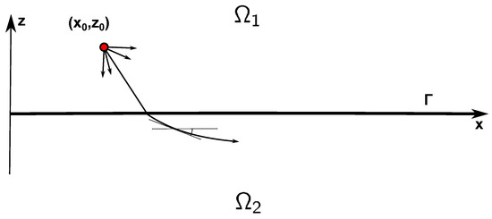
Figure 1.
Geometry of the problem.
Assume that in the half-spaces and acoustic properties of the media are different. In the domain , the sound speed is equal to , while in , the sound speed varies with the depth z according to Equation (1).
In the domains and , the nonstationary acoustic fields (e.g., sound pressure) and satisfy wave equations
where is the Dirac delta function and is the source waveform. The boundary conditions of continuity of the wavefield and its normal derivative are imposed on the interface :
These conditions express continuity of acoustic pressure and normal component of the particle velocity across the interface. Finally, it is assumed that for the wavefield is identically zero
Dispersion Equation
The formulation above is related to a nonstationary process in the waveguide. Let us now consider its time-harmonic counterpart that has the form of a wave traveling in the positive direction of the x axis
where is angular frequency and is the horizontal wavenumber. The solutions of the form (6) (either with the time factor or without it) are usually called normal modes.
If , then by substituting (6) into Equations (2) and (3) and using the interface conditions one can derive [13] the following dispersion relation
where
Here, prime denotes the derivative of function v which is the solution of the Airy equation in the notation proposed by Fock (see [14]).
which has an exponentially decreasing asymptotic in
The well-known integral representation for the function v is given (in terms of more widely used notation, , see https://mathworld.wolfram.com/Airy-FockFunctions.html, accessed 17 October 2022) by
The complex-valued function of two complex variables and is a meromorphic function with respect to the variable in the domain , which has three branch points . Analysis of the analytic properties of the functions comprising a family of solutions to the equation is important for studying the asymptotic behavior of the wavefield (see [15]).
Because the dispersion relation (7) contains special functions, the equation is transcendental. Finding analytical solutions to this equation seems to be impossible, and the numerical study of solutions is a non-trivial task. Let us perform a trick to eliminate the Airy functions in the dispersion Equation (7).
Let be the solution of the dispersion Equation (7). Then, the total derivative of the function with respect to identically equals to zero. Thus, we have a system of equations
where
Using the definition of the Airy function as the solution to , we rewrite the latter equality as
Because and cannot vanish simultaneously, the above identity, together with (see Equation (7)) is a homogeneous system of two linear equations in which the unknowns are and , and the solution of this system of equations exists if the corresponding determinant equals to zero. Note that the determinant of the system under consideration obviously does not contain Airy functions. Omitting some algebra (basically equating the determinant of the system of linear equations to zero), we obtain the Cauchy problem for finding .
Thus, using the functional properties of the Airy functions and the system (8), we significantly simplify the dispersion Equation (7) to a nonlinear first-order ordinary differential equation. We get the following Cauchy problem for finding
The initial condition at can be written as
where is n-th zero of the Airy function .
2.2. Airy Waveguide with the Compact Cross-Section
Let us now consider the 2D nonstationary sound propagation problem of a point source located on the upper boundary (, ) of the waveguide of finite width shown in Figure 2. We now perform a derivation similar to the one from the previous section for a layer of -linear medium bounded by two flat surfaces.
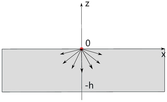
Figure 2.
Geometry of the waveguide.
Let the function satisfy the following equation
As in the previous section, we assume that the sound speed in the medium increases with increasing (i.e., increases in the direction from the boundary downwards)
Let the function U satisfy the Dirichlet boundary conditions at the top and bottom boundaries of the layer
and also satisfy the same initial condition as in the previous section
2.2.1. Dispersion Equation
Again, we introduce the following ansatz
into Equation (13).
Let us find the set of values and for which non-trivial solutions U of the homogeneous counterpart of the problem formulated in Section 2.2 exist. This leads us to
We now change the variables in the latter equation according to the formulae
and obtain an Airy equation as a result.
Passing back to the variable z, we obtain the general solution of Equation (15) in the domain in the following form:
where
and the functions and are two linearly independent solutions to the Airy Equation (16) defined by Fock (see [14]). Let
Then, requiring the fulfillment of the Dirichlet boundary conditions for and , we obtain:
It is obvious that
therefore, for the convenience of subsequent calculations, we introduce new variables:
The system of Equation (19) has non-trivial solutions (a,b) if and only if the corresponding determinant is equal to zero, i.e.,
Equation (20), up to the change of variables, is the required dispersion relation for the considered finite-width waveguide. In the next subsection, the latter equation will be reduced to an initial-value problem for a nonlinear ODE.
2.2.2. Reduction of Equation (20)
We denote the left-hand side of Equation (20) as f, i.e.,
The solutions of the dispersion relation in terms of the variables y and s are the functions satisfying
Let be one of these solutions. Because the Formula (21) is an identity, the total derivative of the function with respect to the parameter s is also a function identically equal to zero:
Obviously, we can differentiate the function in this way any number of times and obtain more identities.
Note that in Equation (20) we have two independent Airy functions and . The aim is to exclude these transcendental functions from the equation. In Equation (20), the two independent Airy functions appear in a combination with two different arguments y and , so there are only four parameters to eliminate. With only one Equation (20), we obviously cannot do this. Combining Equations (21) and (22) we obtain a system of another two equations. Because the second equation of the system is basically a result of differentiation of the first one, we now have eight unknowns instead of two. Indeed, when differentiating, we get the new parameters required to eliminate the terms and .
The good news is that by further differentiation, the number of new parameters to eliminate will not increase and will remain equal to eight. This is easy to see from the equation that is used in the definition of the Airy function.
However, in order to eliminate eight unknown parameters, we must have eight independent equations. Thus, we will have to differentiate Equation (20) seven times in total and combine the resulting new identities with the dispersion equation itself. Already, at the stage of taking the third total derivative, we get cumbersome nonlinear functions, and as a result of the elimination of the resulting system of eight equations, we get a very cumbersome seventh-degree nonlinear differential equation which is difficult to work with.
We come to the conclusion that the trick we managed to perform in the problem with the interface between the two half-planes no longer leads us to a simple and beautiful result. The reason for this problem, which does not occur in the case of the contact of two half-planes, is the presence of two walls (the Dirichlet boundary conditions) of the considered waveguide. In the case of half-planes, the inhomogeneous medium filled a half-plane unbounded from below, and in view of the radiation conditions at infinity, in the corresponding dispersion equation we obtained only one Airy function . In addition, we had only one interface between the media; correspondingly, the interface conditions were imposed only at . This results in the fact that the Airy function in the dispersion relation depends on only one argument. In the case considered here, due to the presence of an additional lower boundary, we have twice as many independent Airy functions and twice as many arguments. That is, unlike the problem with the contact of semi-infinite media, where one differentiation was enough, leading us to a system of two independent equations to eliminate two unknown quantities, now we have four times as many parameters, which makes the task much more difficult.
For the purpose of decreasing the order of the resulting ODE (here it is seven) and its strong nonlinearity, we propose another trick.
Let us introduce three more new functions of two variables y and s:
It is easy to see that the functions , , , and , which are linear combinations of Airy functions and their derivatives, are linearly independent and that their values form a non-trivial set complex numbers at for any complex value of parameter s, i.e., , , , and do not vanish simultaneously for any .
It can be found that the total derivative of of any order can be expressed in terms of , , and . Indeed, the following identities hold (in subsequent calculations, for simplicity, we omit the argument of the form ())
Hence, we come to the conclusion that in order to exclude transcendental functions, it is enough for us to compose and solve a system of four linear equations, the first of which is the dispersion equation itself (more precisely, its counterpart in the variables y and s), and the other three equations are obtained by differentiating the previous ones. That is, in the end, we get a system of equations. Solving this system, we obtain a third-order nonlinear differential equation. Thus, we significantly simplify the nonlinearity of the final equation and reduce its order by four.
Now let us derive the equations of the described system. We already have the first equation, it is the identity
Omitting calculations, we write down the results obtained. The second equation, obtained by differentiating the first one, has the following form
and the third can be written as
Finally, the fourth equation, obtained by taking the third total derivative of the dispersion relation written in the variables y and s has the form
As we will see below, the function in the last formula does not need to be defined.
Because the functions , , , and do not vanish simultaneously for any , then the obtained system of four linear equations is solvable if and only if the determinant of the respective matrix is identically zero for all s. The matrix itself has the following structure (here, the equality is taken into account):
Because , , and are equal to zero, the determinant of the matrix A does not depend on q(y(s),s). Hence, in order to simplify the necessary calculations, we do not provide the expression for q here (according to the argument above).
The determinant of this matrix is easy to calculate:
Substituting the coefficients at , , , and in the equations obtained as a result of differentiation of Equation (20) into the expression (23), we obtain (after some algebra) the desired ODE that must be satisfied by all solutions of the transcendental Equation (20)
This is a nonlinear ODE of the third order.
3. Multi-Layered Waveguide
Let us consider a multi-layered waveguide with the first and last layers being semi-infinite in z.
In the lower half-plane each layer is an -linear medium, while the upper half-plane is a stack of layers with a constant sound speed (see Figure 3). There can be finite jumps of the sound speed across the interfaces between layers, and the boundary conditions of continuity of the wave field and its normal derivative on the interfaces are fulfilled.

Figure 3.
Geometry of the multilayer waveguide.
Note that by adding of interfaces in the lower half-plane, we change the order of the dispersion relation (rewritten as an ODE) and, in a certain sense, enhance its nonlinearity. Thus, having interfaces in the lower half-plane and following the same reduction procedure as in the previous section, we would obtain a nonlinear ODE of the order . However, adding extra boundaries in the upper half-plane (and the respective number of isovelocity layers), we will not change the structure of the dispersion equation and therefore will not affect the order of the differential equation either.
4. Conclusions
We developed a technique for reducing the transcendental dispersion equation to a nonlinear ordinary differential equation using a certain class of diffraction problems as an example. Note that this method is applicable not only to acoustic media with a piecewise -linear sound speed profile resulting in the Airy functions in the dispersion relation but also, for example, to the profiles that result in the function of a parabolic cylinder in the dispersion relation. We believe that even wider classes of the sound speed dependencies on the depth z can be covered by the proposed approach.
In addition to purely theoretical interest, the results of this study can be used to improve the performance of geoacoustic inversion algorithms that require fast computation of horizontal wavenumbers for multiple frequencies. The enhancement can be achieved by solving the spectral problem for the highest frequency involved and then solving the respective nonlinear ODE numerically. Thus, one can obtain the values of both and the respective modal group velocities that can be easily computed as inverse quantities for the right-hand side of ODEs similar to (11). Note that in general it is difficult to find a technique for solving transcendental Equations (such as the dispersion relations) that are both efficient and robust. Therefore, in practice the solution of a nonlinear ODE appears to be a more attractive alternative.
Author Contributions
Conceptualization, A.M., G.Z., P.P.; investigation, A.M., G.Z., writing—original draft preparation, G.Z.; reviewing and editing, G.Z., A.M., P.P. All authors have read and agreed to the published version of the manuscript.
Funding
This study was supported by the Russian Science Foundation, project No. 22-11-00171 (https://rscf.ru/en/project/22-11-00171).
Institutional Review Board Statement
Not applicable.
Informed Consent Statement
Not applicable.
Data Availability Statement
Not applicable.
Conflicts of Interest
The authors declare no conflict of interest.
References
- Landau, L.D.; Lifshitz, E.M. Quantum Mechanics: Non-Relativistic Theory; Elsevier: Amsterdam, The Netherlands, 2013; Volume 3. [Google Scholar]
- Jensen, F.B.; Kuperman, W.A.; Porter, M.B.; Schmidt, H. Computational Ocean Acoustics; Springer Science & Business Media: Berlin/Heidelberg, Germany, 2011. [Google Scholar]
- Petrov, P.; Prants, S.; Petrova, T. Analytical Lie-algebraic solution of a 3D sound propagation problem in the ocean. Phys. Lett. A 2017, 381, 1921–1925. [Google Scholar] [CrossRef]
- Virieux, J.; Farra, V.; Madariaga, R. Ray tracing for earthquake location in laterally heterogeneous media. J. Geophys. Res. Solid Earth 1988, 93, 6585–6599. [Google Scholar] [CrossRef]
- Vallée, O.; Soares, M. Airy Functions and Applications to Physics; World Scientific Publishing Company: Singapore, 2010. [Google Scholar]
- Levy, M. Parabolic Equation Methods for Electromagnetic Wave Propagation; IET: London, UK, 2000. [Google Scholar]
- Warner, G.A.; Dosso, S.E.; Dettmer, J.; Hannay, D.E. Bayesian environmental inversion of airgun modal dispersion using a single hydrophone in the Chukchi Sea. J. Acoust. Soc. Am. 2015, 137, 3009–3023. [Google Scholar] [CrossRef] [PubMed]
- Bonnel, J.; Thode, A.; Wright, D.; Chapman, R. Nonlinear time-warping made simple: A step-by-step tutorial on underwater acoustic modal separation with a single hydrophone. J. Acoust. Soc. Am. 2020, 147, 1897–1926. [Google Scholar] [CrossRef] [PubMed]
- Buldyrev, V.S. An investigation of the Green’s function in a problem of diffraction by a transparent circular cylinder. I. Zhurnal Vychislitel’noi Mat. I Mat. Fiz. 1964, 4, 275–286. [Google Scholar] [CrossRef]
- Buldyrev, V. Interference of short waves in the problem of diffraction by an inhomogeneous cylinder of arbitrary cross section. Izv. Vyssh. Uchebn. Zaved. Radiofiz. 1967, 10, 699–711. [Google Scholar]
- Babič, V.M.; Buldyrev, V.S. Asymptotic Methods in Short-Wavelength Diffraction Theory; Alpha Science International Limited: Oxford, UK, 2009. [Google Scholar]
- Brekhovskikh, L. Waves in Layered Media; Academic Press: Cambridge, MA, USA, 1960. [Google Scholar]
- Zavorokhin, G.; Matskovskiy, A. A Nonstationary Problem of Diffraction of Acoustic Waves from a Point Source by an Interface of Two Half-Planes with Positive Effective Curvature. J. Math. Sci. 2021, 252, 612–618. [Google Scholar] [CrossRef]
- Fock, V.A. Electromagnetic Diffraction and Propagation Problems; Pergamon Press: Oxford, UK, 1965. [Google Scholar]
- Shanin, A.; Knyazeva, K.; Korolkov, A. Riemann surface of dispersion diagram of a multilayer acoustical waveguide. Wave Motion 2018, 83, 148–172. [Google Scholar] [CrossRef]


Publisher’s Note: MDPI stays neutral with regard to jurisdictional claims in published maps and institutional affiliations. |
© 2022 by the authors. Licensee MDPI, Basel, Switzerland. This article is an open access article distributed under the terms and conditions of the Creative Commons Attribution (CC BY) license (https://creativecommons.org/licenses/by/4.0/).