Speed Fluctuation Suppression Strategy of Servo System with Flexible Load Based on Pole Assignment Fuzzy Adaptive PID

Abstract

Flexible load is widely used in servo systems, and will cause nonlinear displacement and vibration of the system and then cause speed fluctuations in the servo system motor. In order to reduce the fluctuation of system velocity, a fuzzy adaptive vibration suppression strategy based on pole assignment is proposed. Firstly, the dynamic model of the flexible-load system is established by using the assumed mode method (AMM) and the Lagrange principle. Then, according to the initial traditional PID parameters, the same real-part pole assignment method is used to improve it. Next, a fuzzy adaptive rule is designed to adjust the PID parameters after pole assignment. Finally, three different control strategies are applied to the servo-driven flexible-load system, three different conditions with the variable as the length of the flexible load are selected for numerical simulation, the output parameters of the system are obtained, and the errors are analyzed. The results show that the fuzzy adaptive PID control strategy based on pole assignment proposed in this paper makes the system have a higher working accuracy, and compared with the traditional PID control method and the improved PID control method, the vibration suppression effect of the system is more obvious, and the stability of the system can be increased by about 10%, which fully demonstrates the effectiveness of the control strategy proposed in this paper.

1. Introduction

In recent years, high-performance industrial robots have been widely used in many high-end application fields such as aerospace exploration, aviation manufacturing, and intelligent assembly [1,2]. In motion control systems such as industrial robots and aerospace mechanism drives, the performance of robotic arms has been continuously improved. The working area is expanded, thus the size of the operating mechanism is increased continuously. In order to further reduce the load of the system, lightweight structural materials with high deadweight ratios are usually selected to improve the running speed and working efficiency [3,4,5]. However, these mechanical arms easily produce elastic deformation and cause corresponding stress in the process of rotating motion. They have typical flexible load characteristics, and can also be referred to as flexible load characteristics for larger load mechanisms. Compared with the rigid load, the characteristics of the flexible load will have a great impact on the motion control of the mechanism, which easily causes low positioning accuracy and system instability caused by the resonance of the system [6,7,8]. Therefore, the study of servo system control can effectively suppress the elastic deformation of the flexible load due to vibration and improve the stability of the system.

In order to realize the motion control of the servo-driven flexible-load system and make the system reach a stable state, the system dynamics model should be established first. At present, many scholars have carried out relevant research, and the dynamic modeling of flexible load mainly includes the hypothetical mode method and finite element method. In [9,10,11], the flexible load is equivalent to the Euler–Bernoulli beam, ignoring its axial and longitudinal deformation in the process of movement, but only considering the transverse deformation. In [12,13,14], the assumed mode method is used to describe the end deflection of flexible loads, and the Lagrange principle is used to establish its dynamic equation. In [15,16,17], the finite element method is used to establish flexible load dynamic models with complex shapes to improve the working accuracy of the system. In [18,19,20,21], Hamilton’s principle is used to calculate the Hamilton function of the system, and the system is modeled in the way of energy. The authors of [22,23] use the theory of mechanical vibration to obtain the partial differential equation of the flexible manipulator, list the vibration boundary conditions, and finally obtain the motion equation of the system.

The servo-driven flexible-load system is a complex nonlinear system with high coupling, and the above modeling methods can accurately describe the dynamics of the system. In the actual working process, the flexibility of the load will have an impact on the rotation speed of the servo system [24,25]. Therefore, it is very important to study the control of the servo-drive system. In the field of high-performance servo drives, the servo control strategy is still dominated by the traditional PID adjustment [26,27]. Therefore, on the basis of the traditional PID adjustment method, the appropriate state feedback is introduced to suppress the resonance caused by the flexibility to the maximum extent. This research is of great value. The authors of [28,29] use the pole assignment strategy to determine the control system parameters and compensate for the arbitrary load torque of the system through a feedforward controller with flexible load torque. The authors of [30] put forward the neural network control with full state feedback and output feedback, which can effectively suppress the elastic vibration of flexible beams. The authors of [31] proposed a robust adaptive fault-tolerant control (FTC) based on radial basis function (RBF), which proved the effectiveness of vibration suppression for rigid-flexible coupled robots under external disturbance and unknown control direction. In [32], an adaptive fuzzy control method is applied to the control of a single-link flexible joint robot, which ensures the stability of the system.

In this paper, the dynamic modeling of the servo-driven flexible-load system is firstly carried out. According to [13,14], the AMM is used to equivalent the flexible load to the Euler–Bernoulli beam, and then the Lagrange principle is used for dynamic modeling. Compared with [26,27], the traditional PID control parameters are improved, and the same real-part pole assignment method is used to adjust them, which improves the system stability to a certain extent. Compared with [28,29], this paper proposes a fuzzy adaptive control strategy on this basis to adjust the PID parameters after tuning, which has a more significant effect on improving the stability of the system. The elastic deformation of the flexible load and the variation of the output torque under three different working conditions are obtained by simulation. The error of the output results when the variable is the length of the flexible load is analyzed, and the effectiveness of the proposed fuzzy adaptive PID control strategy based on pole assignment is verified by numerical simulation.

The rest of this paper is as follows: in Section 2, the dynamic modeling of the servo-driven flexible-load system is carried out by using the AMM and Lagrange principle. In Section 3, a fuzzy adaptive PID control strategy based on pole assignment is proposed. In Section 4, the simulation results are given and the error analysis is carried out. Section 5 draws the conclusion.

2. Modeling of a Servo System with Flexible Load

There is a kind of flexible load widely in servo systems, such as space manipulators, industrial robots, and so on. In order to facilitate the establishment of the mathematical model of the flexible load driven by the motor, the system model should be simplified and equivalent to the central rigid body–cantilever system. The cantilever is equivalent to a flexible load, and the cantilever can be equivalent to a flexible link. Ignoring the transmission ratio of the system and the joint flexibility of the flexible arm, the servo-driven single flexible-load system model as shown in Figure 1 was established. When the system moves in a wide range, the flexural vibration of the flexible link is much more obvious in the transverse direction than that in the longitudinal direction. As a result, the longitudinal vibration can be ignored. Therefore, the influence of the longitudinal deformation on the system motion is not considered under general circumstances. In the modeling process, the flexible link is equivalent to the Euler–Bernoulli beam, which has the following assumptions:

• The shear deformation and axial deformation are ignored, and only the deformation caused by transverse vibration is considered;
• The transverse deformation is small deformation;
• The beam is much longer than its cross-section size.

In Figure 1b, the static coordinate $X_s{O}_s{Y}_s$ is established on the motor shaft and the dynamic coordinate $X_1{O}_1{Y}_1$ is established on the flexible connecting rod. T_S is the electromagnetic torque of the motor; ${\theta }_{\mathrm{s}}\left(t\right)$ represents the rotation angle of the servo motor under the action of torque T_S; $\delta \left(x,t\right)$ represents the deformation caused by the transverse vibration of the flexible connecting rod, that is, the deflection of the cantilever beam at x; and $\delta \left(x,t\right)$ is a two-dimensional function of the position x and time t of the load section.

According to the AMM, the deflection of the flexible connecting rod at x can be obtained as shown in Equation (1):

$$\delta \left(x,t\right)={{\displaystyle \sum }}_{i=1}^{\infty }{\varphi }_i\left(x\right){\mathit{\mu }}_i\left(t\right)={\varphi }^{\mathrm{T}}\mathit{\mu },$$

(1)

where ${\varphi }_i\left(x\right)$ is the modal shape function; ${\mathit{\mu }}_i\left(t\right)$ is the modal coordinate.

At the same time, according to the vibration theory, the partial differential equation of the transverse vibration of the flexible load can be obtained after it is equivalent to the Euler–Bernoulli beam, which is expressed as Equation (2):

$$\frac{{\partial }^2}{\partial x^2}\left[\mathit{EI}\left(x\right)\frac{{\partial }^2\delta \left(x,t\right)}{\partial x^2}\right]+\mathit{\rho }\left(x\right)\mathit{A}\left(x\right)\frac{{\partial }^2\delta \left(x,t\right)}{\partial t^2}=\mathit{P}\left(x,t\right),$$

(2)

where $\mathit{EI}\left(x\right)$ represents the flexural stiffness of the flexible load; $\mathit{\rho }\left(x\right)$ represents the unit line density of the flexible load; $\mathit{A}\left(x\right)$ represents the unit cross-sectional area of the flexible load; $\mathit{P}\left(x,t\right)$ represents the distributed force acting on the flexible load.

The flexible load can be regarded as a cantilever beam with one end free and one end fixed. Ignoring the force and mass concentration at the end of the flexible load, the boundary conditions can be obtained as follows:

$$\{\begin{array}{c}\begin{array}{c}\delta \left(0,t\right)=0\\ \frac{\partial \delta \left(0,t\right)}{\partial x}=0\\ \mathit{EI}\left(x\right)\frac{{\partial }^2\delta \left(l,t\right)}{\partial x^2}=0\prime \end{array}\\ \mathit{EI}\left(x\right)\frac{{\partial }^3\delta \left(l,t\right)}{\partial x^3}=0\end{array}$$

(3)

If the flexible load is assumed to be uniform and the external force is ignored, that is, $\mathit{EI}\left(x\right)$, $\mathit{\rho }\left(x\right)$, and $\mathit{A}\left(x\right)$ can be represented by constant values, namely $\mathit{EI}$, $\mathit{\rho }$, and $\mathit{A}$, and the distributed force is $\mathit{P}\left(x,t\right)=0$. Next, the vibration mode shape function ${\varphi }_i\left(x\right)$ is solved, and Equation (2) can be arranged as follows:

$$\frac{{\partial }^2}{\partial x^2}\left[\mathit{EI}\frac{{\partial }^2\delta \left(x,t\right)}{\partial x^2}\right]+\mathit{\rho }\mathit{A}\frac{{\partial }^2\delta \left(x,t\right)}{\partial t^2}=0,$$

(4)

Using the method of separation of variables to solve, substituting Equation (1) into Equation (4), Equation (5) can be obtained as:

$$\mathit{EI}\varphi \prime \prime \prime \prime \left(x\right)\mathit{\mu }\left(t\right)+\mathit{\rho }\mathit{A}\varphi \left(x\right)\mathit{\mu }\prime \prime \prime \prime \left(t\right)=0,$$

(5)

Equation (5) is changed into Equation (6), and it can be obtained that:

$$\frac{\ddot{\mathit{\mu }}\left(t\right)}{\mathit{\mu }\left(t\right)}=-\frac{\mathit{EI}}{\mathit{\rho }\mathit{A}}·\frac{{\varphi }^{\prime \prime \prime \prime }\left(x\right)}{\varphi \left(x\right)},$$

(6)

In Equation (6), the left side is only related to t and the right side is only related to x, so it can only be equal to a constant. This constant is denoted as $-{\mathit{\omega }}^2$, and Equation (7) can be obtained:

$$\{\begin{array}{c}\frac{{\mathrm{d}}^2\mathit{\mu }\left(t\right)}{\mathrm{d}{t}^2}+{\mathit{\omega }}^2\mathit{\mu }\left(t\right)=0\\ \mathit{EI}{\varphi }^{\prime \prime \prime \prime }\left(x\right)-{\mathit{\omega }}^2\mathit{\rho }\mathit{A}\varphi \left(x\right)=0\end{array},$$

(7)

Finally:

$${\varphi }^{\prime \prime \prime \prime }\left(x\right)-\frac{{\mathit{\omega }}^2\mathit{\rho }\mathit{A}}{\mathit{EI}}\varphi \left(x\right)={\varphi }^{\prime \prime \prime \prime }\left(x\right)-{\alpha }^4\varphi \left(x\right)=0,$$

(8)

Therefore, the modal function and frequency of flexural vibration of flexible load are determined according to the above equation, and the characteristic equation can be obtained, as shown in Equation (9):

$${\varphi }_i\left(e^{\lambda x}\right),$$

(9)

Then, the characteristic root of this equation can be solved by the characteristic Equation (9), as shown in Equation (10):

$$\{\begin{array}{c}{\lambda }^4-{\alpha }^4=0\\ {\lambda }_{1,2}=\pm \alpha ,\\ {\lambda }_{3,4}=\pm i\alpha \end{array}$$

(10)

Therefore, the modal function $\varphi \left(x\right)$ can be expressed as Equation (11):

$${\varphi }_i\left(x\right)={\Psi }_1{e}^{\alpha x}+{\Psi }_2{e}^{-\alpha x}+{\Psi }_3{e}^{i\alpha x}+{\Psi }_4{e}^{-i\alpha x},$$

(11)

The above equation can be transformed into Equation (12):

$${\varphi }_i\left(x\right)={\Psi }_1\sin \alpha x+{\Psi }_2\cos \alpha x+{\Psi }_3\mathrm{sh}\alpha x+{\Psi }_4\mathrm{ch}\alpha x,$$

(12)

In Equation (12), the boundary conditions can be used to solve the integration constants ${\Psi }_1$, ${\Psi }_2$, ${\Psi }_3$, and ${\Psi }_4$.

According to Equation (7), the solutions of modal coordinate $\mathit{\mu }\left(t\right)$ and lateral vibration displacement $\delta \left(x,t\right)$ of flexible load are obtained, which are expressed as Equations (13) and (14):

$$\mathit{\mu }\left(t\right)=H\sin \left(\mathit{\omega }t+\mathit{\phi }\right),$$

(13)

$$\delta \left(x,t\right)=R\sin \left(\mathit{\omega }t+\mathit{\phi }\right),$$

(14)

In Equation (14), R can be expressed as in Equation (15):

$$R={\chi }_1\sin \alpha x+{\chi }_2\cos \alpha x+{\chi }_3\mathrm{sh}\alpha x+{\chi }_4\mathrm{ch}\alpha x,$$

(15)

Among them, ${\chi }_i\left(i=1,\cdots ,4\right)$, $\mathit{\omega }$ and $\mathit{\phi }$ are undetermined coefficients, which can be determined according to the initial and boundary conditions of vibration. Meanwhile, the frequency equation can be obtained according to the boundary conditions, as shown in Equation (16):

$$\cos \alpha l+\mathrm{ch}\alpha l=-1,$$

(16)

The natural frequency of the flexible load is shown in the following equation:

$${\mathit{\omega }}_i={\alpha }_i^2\sqrt{\frac{\mathit{EI}}{\mathit{\rho }\mathit{A}},}$$

(17)

The modal function corresponding to ${\mathit{\omega }}_i$ can be expressed as Equation (18):

$${\varphi }_i\left(x\right)=\mathrm{ch}{\alpha }_{i}x-\cos {\alpha }_{i}x-{\zeta }_i\left(\mathrm{sh}{\alpha }_{i}x-\sin {\alpha }_{i}x\right),$$

(18)

In Equation (18), the expression of ${\zeta }_i$ is shown in Equation (19):

$${\zeta }_i=\frac{\mathrm{sh}{\alpha }_{i}l-\sin {\alpha }_{i}l}{\mathrm{ch}{\alpha }_{i}l+\cos {\alpha }_{i}l},$$

(19)

where ${\alpha }_i$ is the eigenvalue of the flexible load, which is the root of Equation (16), and its solution is expressed in Equation (20):

$${\alpha }_i=\frac{2i-1}{l}\pi \left(i=1,2,\cdots \right),$$

(20)

Therefore, the first three-order eigenroot values of the flexible load can be calculated, as shown in

Table 1. Eigenroot values of the first three orders of flexible loads.

The Characteristic Root  ${\mathit{\alpha }}_{\mathit{i}}$	${\alpha }_1$	${\alpha }_2$	${\alpha }_3$
The Values	1.875	4.694	7.855

below.

The motion of the flexible load in the horizontal plane can be regarded as a large range of rigid body motion superimposed on a small range of elastic deformation motion. Therefore, the vector of any point on the flexible load can be expressed as shown in Equation (21):

$$\begin{array}{c}{\mathit{r}}^{\mathrm{T}}=\left[X,Y\right]\\ \{\begin{array}{c}X=x\cos {\theta }_s\left(t\right)-\delta \left(x,t\right)\sin {\theta }_s\left(t\right),\\ Y=x\sin {\theta }_s\left(t\right)+\delta \left(x,t\right)\cos {\theta }_s\left(t\right)\end{array}\end{array}$$

(21)

Therefore, the kinetic energy of the flexible load can be obtained as:

$$\mathit{T}=\frac{1}{2}\mathit{\rho }\mathit{A}{{\displaystyle \int }}_0^1{\dot{\mathit{r}}}^{\mathrm{T}}\dot{\mathit{r}}\mathrm{d}x=\frac{1}{2}\mathit{\rho }\mathit{A}{{\displaystyle \int }}_0^1\left({\dot{X}}^2+{\dot{Y}}^2\right)\mathrm{d}x,$$

(22)

In Equation (22),

$${\dot{\mathit{r}}}^{\mathrm{T}}\dot{\mathit{r}}=\left(x^2+{\delta }^2\left(x,t\right)\right){\dot{\theta }}_s^2\left(t\right)+{\left(\frac{\partial \delta \left(x,t\right)}{\partial t}\right)}^2+2x{\dot{\theta }}_s^2\left(t\right)\frac{\partial \delta \left(x,t\right)}{\partial t},$$

(23)

Assuming that the flexible load moves in the horizontal plane, its potential energy is generated only by elastic deformation, so its elastic potential energy can be obtained as:

$$\mathit{V}=\frac{1}{2}\mathit{EI}{{\displaystyle \int }}_0^1\frac{{\partial }^2\delta \left(x,t\right)}{\partial x^2}\mathrm{d}x,$$

(24)

According to the Lagrange equation, the kinetic energy and potential energy of the flexible load are substituted into it, and the dynamic equation of the system can be obtained:

$$\frac{\mathrm{d}}{\mathrm{d}t}\left(\frac{\partial \mathit{T}}{\partial \dot{\overline{{\mathit{q}}_i}}}\right)-\frac{\partial \mathit{T}}{\partial \overline{{\mathit{q}}_i}}+\frac{\partial \mathit{V}}{\partial \overline{{\mathit{q}}_i}}={\mathit{Q}}_i,$$

(25)

where $\overline{{\mathit{q}}_i}\left(1,2,\cdots ,n+1\right)$ represents the mechanical angle ${\theta }_s$ of the motor and the ith mode coordinate ${\mathit{\mu }}_i\left(t\right)$ of the flexible load, and ${\mathit{Q}}_i$ represents the generalized force exerted by the system. Therefore, Equation (26) can be obtained:

$$\{\begin{array}{c}\frac{\mathrm{d}}{\mathrm{d}t}\left(\frac{\partial \mathit{T}}{\partial {\dot{\theta }}_s\left(t\right)}\right)-\frac{\partial \mathit{T}}{\partial {\theta }_s\left(t\right)}+\frac{\partial \mathit{V}}{\partial {\theta }_s\left(t\right)}={\mathit{T}}_s\\ \frac{\mathrm{d}}{\mathrm{d}t}\left(\frac{\partial \mathit{T}}{\partial {\mathit{\mu }}_i\left(t\right)}\right)-\frac{\partial \mathit{T}}{\partial {\mathit{\mu }}_i\left(t\right)}+\frac{\partial \mathit{V}}{\partial {\mathit{\mu }}_i\left(t\right)}=0\end{array},$$

(26)

By rearranging Equation (26) and removing the nonlinear term, Equation (27) can be obtained:

$$\{\begin{array}{c}\mathit{\rho }\mathit{A}{\ddot{\theta }}_s\left(t\right){{\displaystyle \int }}_0^l{x}^2\mathrm{d}x+\mathit{\rho }\mathit{A}{{\displaystyle \sum }}_{i=1}^{\infty }{\ddot{\mathit{\mu }}}_i\left(t\right){{\displaystyle \int }}_0^{l}x{\varphi }_i\mathrm{d}x={\mathit{T}}_s\\ {{\displaystyle \sum }}_{i=1}^{\infty }{\ddot{\mathit{\mu }}}_i\left(t\right)+\mathit{\rho }\mathit{A}{\ddot{\theta }}_s\left(t\right){{\displaystyle \int }}_0^{l}x{\varphi }_i\mathrm{d}x+{\mathit{\Omega }}_i{\displaystyle \sum }_{i=1}^{\infty }{\mathit{\mu }}_i\left(t\right)=0\end{array},$$

(27)

Finally, Equation (27) is reorganized into Equation (28):

$$\{\begin{array}{c}{\ddot{\theta }}_s\left(t\right){\mathit{I}}_a+{\mathit{F}}_{ai}^{\mathrm{T}}{\ddot{\mathit{\mu }}}_i\left(t\right)={\mathit{T}}_s\\ {\ddot{\mathit{\mu }}}_i\left(t\right)+2\mathit{\xi }{\mathit{\Omega }}_i{\dot{\mathit{\mu }}}_i\left(t\right)+{\mathit{\Omega }}_i^2{\mathit{\mu }}_i\left(t\right)+{\ddot{\theta }}_s{\mathit{F}}_{ai}=0\end{array},$$

(28)

In Equation (28), ${\xi }_i$ is the damping coefficient matrix of each vibration mode, and Equations (29)–(34) are established:

$${\mathit{\mu }}_i\left(t\right)=\left[{\mathit{\mu }}_1\left(t\right) {\mathit{\mu }}_2\left(t\right) \cdots {\mathit{\mu }}_n\left(t\right)\right],$$

(29)

$${\mathit{I}}_a=\mathit{\rho }\mathit{A}{{\displaystyle \int }}_0^l{x}^2\mathrm{d}x,$$

(30)

$${\mathit{F}}_{ai}={{\displaystyle \int }}_0^l\mathit{\rho }\mathit{A}x{\varphi }_i\left(x\right)\mathrm{d}x,$$

(31)

$${\mathit{F}}_a={\left[{\mathit{F}}_{a1} {\mathit{F}}_{a2} \cdots {\mathit{F}}_{an}\right]}^{\mathrm{T}},$$

(32)

$${\mathit{\Omega }}_i^2=diag\left({\omega }_1^2 , {\omega }_2^2 , \cdots ,{\omega }_n^2 \right),$$

(33)

$${\theta }_m\left(t\right)={\theta }_s\left(t\right)+{{\displaystyle \sum }}_{i=1}^n{\mathit{F}}_{ai}{\mathit{\mu }}_i\left(t\right),$$

(34)

In Equation (34), ${\theta }_m\left(t\right)$ is the end position of the flexible load.

If only the first mode of the system vibration is considered, the modal coupling coefficient vector ${\mathit{F}}_a$ and the resonant frequency matrix $\mathit{\Omega }$ will be scalars, and finally, the simplified dynamic equation of the servo-driven flexible-load system can be obtained, as shown in Equation (35):

$$\{\begin{array}{c}{\ddot{\theta }}_s\left(t\right){\mathit{I}}_a+{\mathit{F}}_{a1}^{\mathrm{T}}{\ddot{\mathit{\mu }}}_1\left(t\right)={\mathit{T}}_s\\ {\ddot{\mathit{\mu }}}_1\left(t\right)+2\mathit{\xi }{\mathit{\Omega }}_1{\dot{\mathit{\mu }}}_1\left(t\right)+{\mathit{\Omega }}_1^2{\mathit{\mu }}_1\left(t\right)+{\ddot{\theta }}_s{\mathit{F}}_{a1}=0\end{array},$$

(35)

Therefore, the equation of the state of the system can be expressed as:

$$\left[\begin{array}{c}{\dot{\theta }}_s\\ \dot{\mathit{\mu }}\left(t\right)\\ {\ddot{\theta }}_s\\ \ddot{\mathit{\mu }}\left(t\right)\end{array}\right]=\left[\begin{array}{cccc}0& 0& 1& 0\\ 0& 0& 0& 1\\ 0& -\frac{{\mathit{\Omega }}_1^2{\mathit{F}}_{a1}^{\mathrm{T}}}{{\mathit{F}}_{a1}^{\mathrm{T}}{\mathit{F}}_{a1}-{\mathit{I}}_a}& 0& -\frac{2{\mathit{\Omega }}_1\mathit{\xi }{\mathit{F}}_{a1}^{\mathrm{T}}}{{\mathit{F}}_{a1}^{\mathrm{T}}{\mathit{F}}_{a1}-{\mathit{I}}_a}\\ 0& \frac{{\mathit{\Omega }}_1^2{\mathit{I}}_a}{{\mathit{F}}_{a1}^{\mathrm{T}}{\mathit{F}}_{a1}-{\mathit{I}}_a}& 0& \frac{2{\mathit{I}}_a{\mathit{\Omega }}_1\mathit{\xi }}{{\mathit{F}}_{a1}^{\mathrm{T}}{\mathit{F}}_{a1}}\end{array}\right]\left[\begin{array}{c}{\theta }_s\\ \mathit{\mu }\left(t\right)\\ {\dot{\theta }}_s\\ \dot{\mathit{\mu }}\left(t\right)\end{array}\right]+\left[\begin{array}{cccc}0& 0& 0& 0\\ 0& 0& 0& 0\\ -\frac{1}{{\mathit{F}}_{a1}^{\mathrm{T}}{\mathit{F}}_{a1}-{\mathit{I}}_a}& 0& 0& 0\\ \frac{{\mathit{F}}_{a1}}{{\mathit{F}}_{a1}^{\mathrm{T}}{\mathit{F}}_{a1}-{\mathit{I}}_a}& 0& 0& 0\end{array}\right]\left[\begin{array}{c}{\mathit{T}}_s\\ 0\\ 0\\ 0\end{array}\right]$$

(36)

According to the state equation of the system, the transfer function of the system can be obtained as:

$$\frac{{\omega }_s\left(s\right)}{{\mathit{T}}_s\left(s\right)}=\frac{1}{s}·\frac{1}{{\mathit{I}}_a-\frac{{\mathit{F}}_{a1}^2}{s^2+2\mathit{\xi }{\mathit{\Omega }}_{1}s+{\mathit{\Omega }}_1^2}},$$

(37)

Therefore, the transfer function of the motor angle to the system can be obtained as:

$$\frac{{\theta }_s\left(s\right)}{{\mathit{T}}_s\left(s\right)}=\frac{s^2+2\mathit{\xi }{\mathit{\Omega }}_{1}s+{\mathit{\Omega }}_1^2}{\left({\mathit{I}}_a-{\mathit{F}}_{a1}^{\mathrm{T}}{\mathit{F}}_{a1}\right)s^4+2{\mathit{I}}_a\mathit{\xi }{\mathit{\Omega }}_1{s}^3+{\mathit{I}}_a{\mathit{\Omega }}_1^2{s}^2},$$

(38)

Further, according to Equations (34) and (38), the end position of flexible load can be expressed as:

$${\theta }_m\left(t\right)={\theta }_s\left(t\right)+{\mathit{F}}_{ai}{\mathit{\mu }}_i\left(t\right),$$

(39)

3. System Control Policy and Parameter Tuning

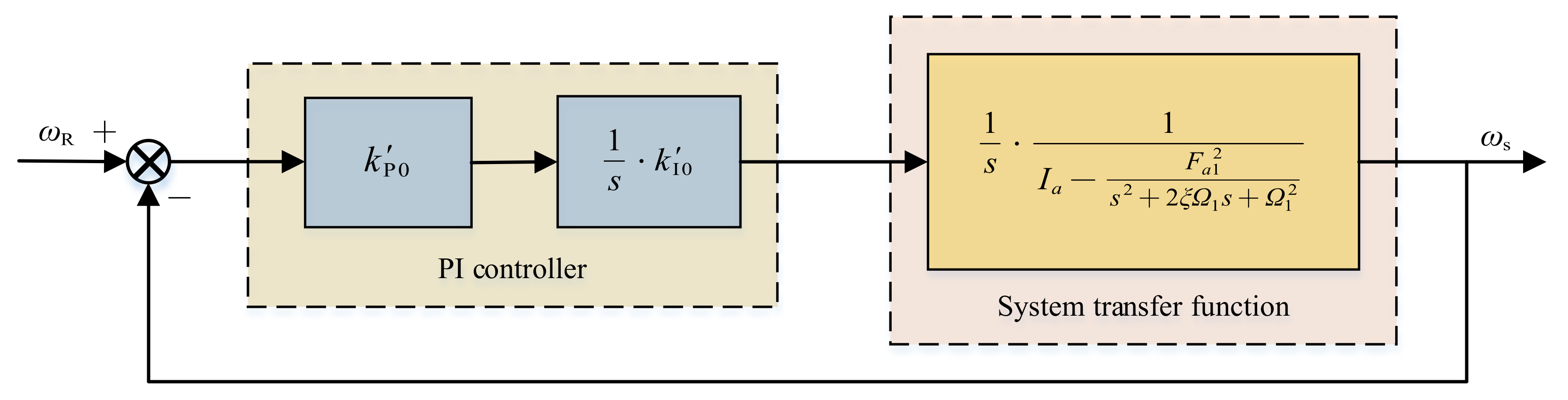
3.1. Design of Servo System Controller Considering Speed Loop

In a servo system, there are three loops for motor control, which are the speed loop, position loop, and current loop. When adjusting the system, the traditional method is to use a PID controller to adjust. When the PID controller is adjusting the servo system, the control bandwidths of the current loop and the speed loop are quite different. Additionally, the system bandwidth of the current loop is usually much larger than the flexible mode frequency. Therefore, it is considered that the current loop has completed the adjustment task when the speed loop is adjusted. Therefore, the influence of the current loop in the servo system is ignored and regarded as constant 1, so that only the influence of the speed loop is considered.

If only the first mode is considered, the following standard form control block diagram of the system speed loop can be obtained when the PI controller is used to adjust the system speed loop, as shown in Figure 2.

Without considering the influence of friction factors, the closed-loop transfer function of the system when the PI controller is used for adjustment can be obtained from the system transfer function of Equation (38), as shown in Equations (40)–(42):

$$\frac{{\omega }_s}{{\omega }_R}=\frac{\left(k_{\mathrm{P}0}^{\prime }s+k_{\mathrm{I}0}^{\prime }\right)\left(s^2+2{\mathit{\Omega }}_1\mathit{\xi }s+{\mathit{\Omega }}_1^2\right)}{\mathrm{M}},$$

(40)

$$\mathrm{M}=\left({\mathit{I}}_a-{\mathit{F}}_{a1}^2\right)s^4+2{\mathit{I}}_a{\mathit{\Omega }}_1\mathit{\xi }{s}^3+{\mathit{I}}_a{\mathit{\Omega }}_1^2{s}^2+\left(k_{\mathrm{P}0}^{\prime }s+k_{\mathrm{I}0}^{\prime }\right)\left(s^2+2{\mathit{\Omega }}_1\mathit{\xi }s+{\mathit{\Omega }}_1^2\right),$$

(41)

In Equations (40) and (42), M is Equation (41), expressed as the denominator form of Equation (40), where $k_{\mathrm{P}0}^{\prime }$ represents the proportional link parameter in the PI controller; $k_{\mathrm{I}0}^{\prime }$ represents the integral link parameter in the PI controller.

In this paper, the Ziegler–Nichols method is firstly used to determine the initial traditional PID parameters, and then the pole assignment method is used to adjust the traditional PI parameters. By referring to the method proposed in [29], Equation (41) is rewritten into the form of Equation (42):

$$\left({\mathit{I}}_a-{\mathit{F}}_{a1}^2\right)s^4+2{\mathit{I}}_a{\mathit{\Omega }}_1\mathit{\xi }{s}^3+{\mathit{I}}_a{\mathit{\Omega }}_1^2{s}^2+\left(k_{\mathrm{P}0}^{\prime }s+k_{\mathrm{I}0}^{\prime }\right)\left(s^2+2{\mathit{\Omega }}_1\mathit{\xi }s+{\mathit{\Omega }}_1^2\right)=\left({\mathit{I}}_a-{\mathit{F}}_{a1}^2\right)\left(s^2+2{\mathit{\xi }}_1^{*2}{\omega }_a^{*}s+{\omega }_a^{*2}\right)\left(s^2+2{\mathit{\xi }}_2^{*2}{\omega }_b^{*}s+{\omega }_b^{*2}\right),$$

(42)

Make:

$$\frac{1}{{\mathit{I}}_a-{\mathit{F}}_{a1}^2}=\mathrm{N},$$

(43)

By combining Equation (42) with Equation (43), Equation (44) can be obtained as follows:

$$s^4+\left(k_{\mathrm{P}0}^{\prime }+2{\mathit{I}}_a{\mathit{\Omega }}_1\mathit{\xi }\right)\mathrm{N}{s}^3+\left(2k_{\mathrm{P}0}^{\prime }{\mathit{\Omega }}_1\mathit{\xi }s+k_{\mathrm{I}0}^{\prime }+{\mathit{I}}_a{\mathit{\Omega }}_1^2\right)\mathrm{N}{s}^2+\left(k_{\mathrm{P}0}^{\prime }{\mathit{\Omega }}_1^2+2k_{\mathrm{I}0}^{\prime }{\mathit{\Omega }}_1\mathit{\xi }\right)\mathrm{N}s+k_{\mathrm{I}0}^{\prime }{\mathit{\Omega }}_1^2\mathrm{N}=\left(s^2+2{\mathit{\xi }}_1^{*2}{\omega }_a^{*}s+{\omega }_a^{*2}\right)\left(s^2+2{\mathit{\xi }}_2^{*2}{\omega }_b^{*}s+{\omega }_b^{*2}\right)$$

(44)

where the natural frequencies of poles are expressed as ${\omega }_a^{*}$ and ${\omega }_b^{*}$; the damping coefficients of the poles are expressed as ${\mathit{\xi }}_1^{*}$ and ${\mathit{\xi }}_2^{*}$. Thus, after ignoring the damping coefficient $\mathit{\xi }$ of the system, the expressions of the proportional link parameter $k_{\mathrm{P}0}^{\prime }$ and the integral link parameter $k_{\mathrm{I}0}^{\prime }$ are:

$$k_{\mathrm{P}0}^{\prime }=\frac{2{\mathit{\xi }}_1^{*}{\omega }_a^{*}+2{\mathit{\xi }}_2^{*}{\omega }_b^{*}}{\mathrm{N}},$$

(45)

$$k_{\mathrm{I}0}^{\prime }=\frac{{\omega }_a^{*}{\omega }_b^{*}}{\mathrm{N}{\mathit{\Omega }}_1^2},$$

(46)

Therefore, Equations (47)–(50) hold, where the position of the zero pole of the system is limited by Equations (49) and (50):

$${\omega }_a^{*2}{\omega }_b^{*2}=\frac{k_{\mathrm{I}0}^{\prime }{\mathit{\Omega }}_1^2}{\mathrm{N}},$$

(47)

$$2{\mathit{\xi }}_1^{*}{\omega }_a^{*}+2{\mathit{\xi }}_2^{*}{\omega }_b^{*}=\frac{k_{\mathrm{P}0}^{\prime }}{\mathrm{N}},$$

(48)

$$2{\mathit{\xi }}_1^{*}{\omega }_a^{*}{\omega }_b^{*2}+2{\mathit{\xi }}_2^{*}{\omega }_b^{*}{\omega }_a^{*2}=\frac{k_{\mathrm{P}0}^{\prime }{\mathit{\Omega }}_1^2}{\mathrm{N}},$$

(49)

$${\omega }_a^{*2}+{\omega }_b^{*2}+4{\mathit{\xi }}_1^{*}{\mathit{\xi }}_2^{*}{\omega }_a^{*}{\omega }_b^{*}=\frac{k_{\mathrm{I}0}^{\prime }+{\mathit{I}}_a{\mathit{\Omega }}_1^2}{\mathrm{N}},$$

(50)

3.2. The Same Real-Part Pole Assignment Method Is Used to Set PI Parameters

The closed-loop transfer function of the system has the same damping coefficient, that is, the pole assignment method with the same real part. As shown in Figure 3, in the distribution of zero and the pole of this pole assignment method, let the four poles have the same real part, so that the zero position ${\mathit{\xi }}_1^{*}$ and ${\mathit{\xi }}_2^{*}$ can move along the dashed path of $-{\mathit{\xi }}_1^{*}{\omega }_a^{*}=-{\mathit{\xi }}_2^{*}{\omega }_b^{*}$.

Substituting $-{\mathit{\xi }}_1^{*}{\omega }_a^{*}=-{\mathit{\xi }}_2^{*}{\omega }_b^{*}$ into Equations (49) and (50), we can obtain:

$${\omega }_a^{*2}+{\omega }_b^{*2}=2{\mathit{\Omega }}_1^2,$$

(51)

$${\left({\omega }_a^{*2}+{\mathit{\Omega }}_1^2\left(2{\mathit{\xi }}_1^{*}-1\right)\right)}^2={\mathit{\Omega }}_1^4\left(4{\mathit{\xi }}_1^{*4}-4{\mathit{\xi }}_1^{*2}+\frac{{\mathit{F}}_{a1}^2}{{\mathit{I}}_a-{\mathit{F}}_{a1}^2}\right),$$

(52)

So, the expressions for ${\omega }_a^{*}$ and ${\omega }_b^{*}$ are:

$$\{\begin{array}{c}{\omega }_a^{*}={\mathit{\Omega }}_1\sqrt{1-2{\mathit{\xi }}_1^{*2}+\sqrt{4{\mathit{\xi }}_1^{*4}-4{\mathit{\xi }}_1^{*2}+\frac{{\mathit{F}}_{a1}^2}{{\mathit{I}}_a-{\mathit{F}}_{a1}^2}}}\\ {\omega }_b^{*}={\mathit{\Omega }}_1\sqrt{1+2{\mathit{\xi }}_1^{*2}-\sqrt{4{\mathit{\xi }}_1^{*4}-4{\mathit{\xi }}_1^{*2}+\frac{{\mathit{F}}_{a1}^2}{{\mathit{I}}_a-{\mathit{F}}_{a1}^2}}}\end{array},$$

(53)

According to Equation (53), the expressions of parameters $k_{\mathrm{P}}^{\prime }$ and $k_{\mathrm{I}}^{\prime }$ can be obtained as:

$$\{\begin{array}{c}{k}_{\mathrm{P}}^{\prime }=4\left({\mathit{I}}_a-{\mathit{F}}_{a1}^2\right){\mathit{\xi }}_1^{*}{\mathit{\Omega }}_1\sqrt{1-2{\mathit{\xi }}_1^{*2}+\sqrt{4{\mathit{\xi }}_1^{*4}-4{\mathit{\xi }}_1^{*2}+\frac{{\mathit{F}}_{a1}^2}{{\mathit{I}}_a-{\mathit{F}}_{a1}^2}}}\\ k_{\mathrm{I}}^{\prime }=\left({\mathit{I}}_a-{\mathit{F}}_{a1}^2\right)\sqrt{1-{\left(2{\mathit{\xi }}_1^{*2}-\sqrt{4{\mathit{\xi }}_1^{*4}-4{\mathit{\xi }}_1^{*2}+\frac{{\mathit{F}}_{a1}^2}{{\mathit{I}}_a-{\mathit{F}}_{a1}^2}}\right)}^2}\end{array},$$

(54)

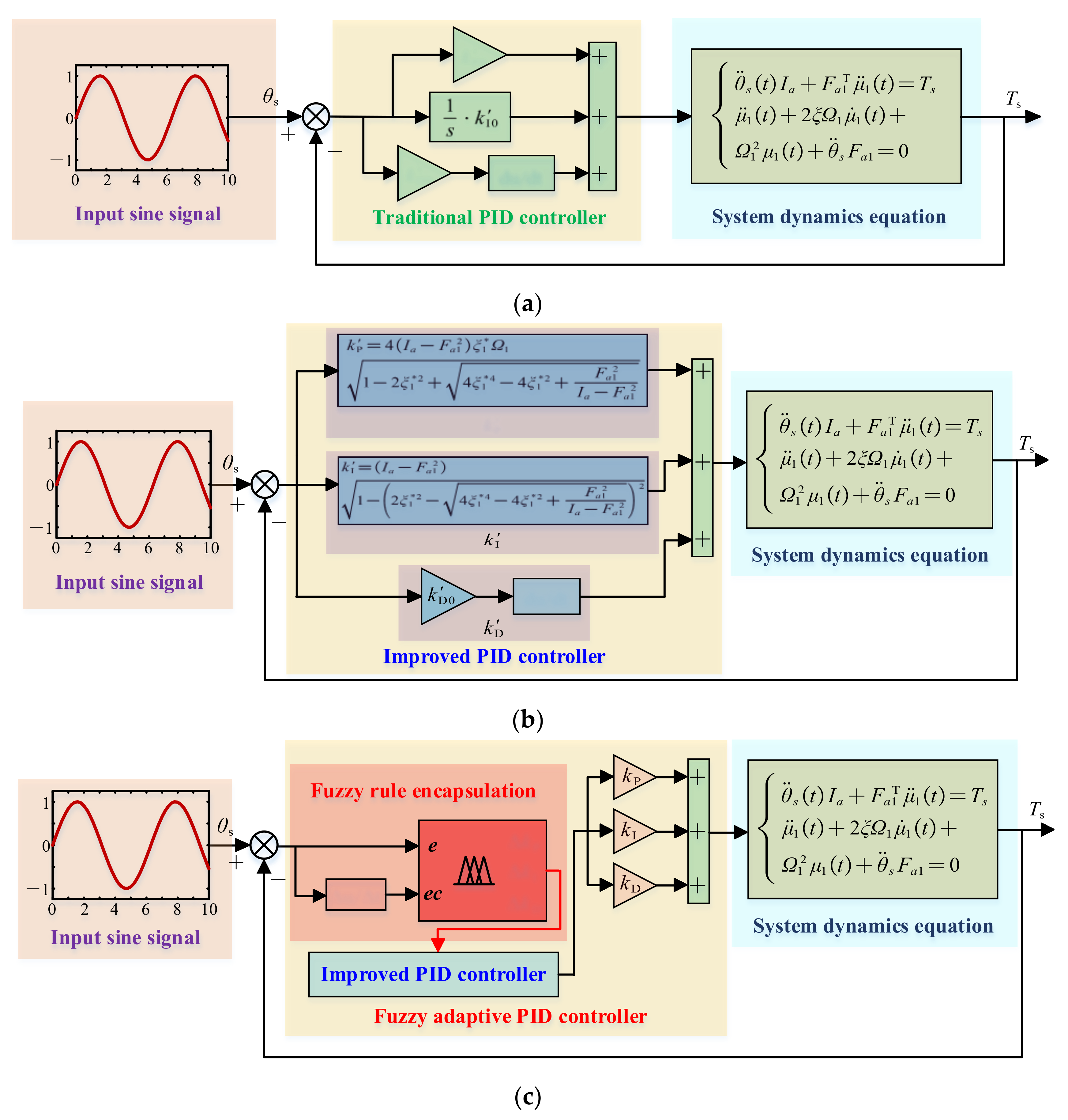
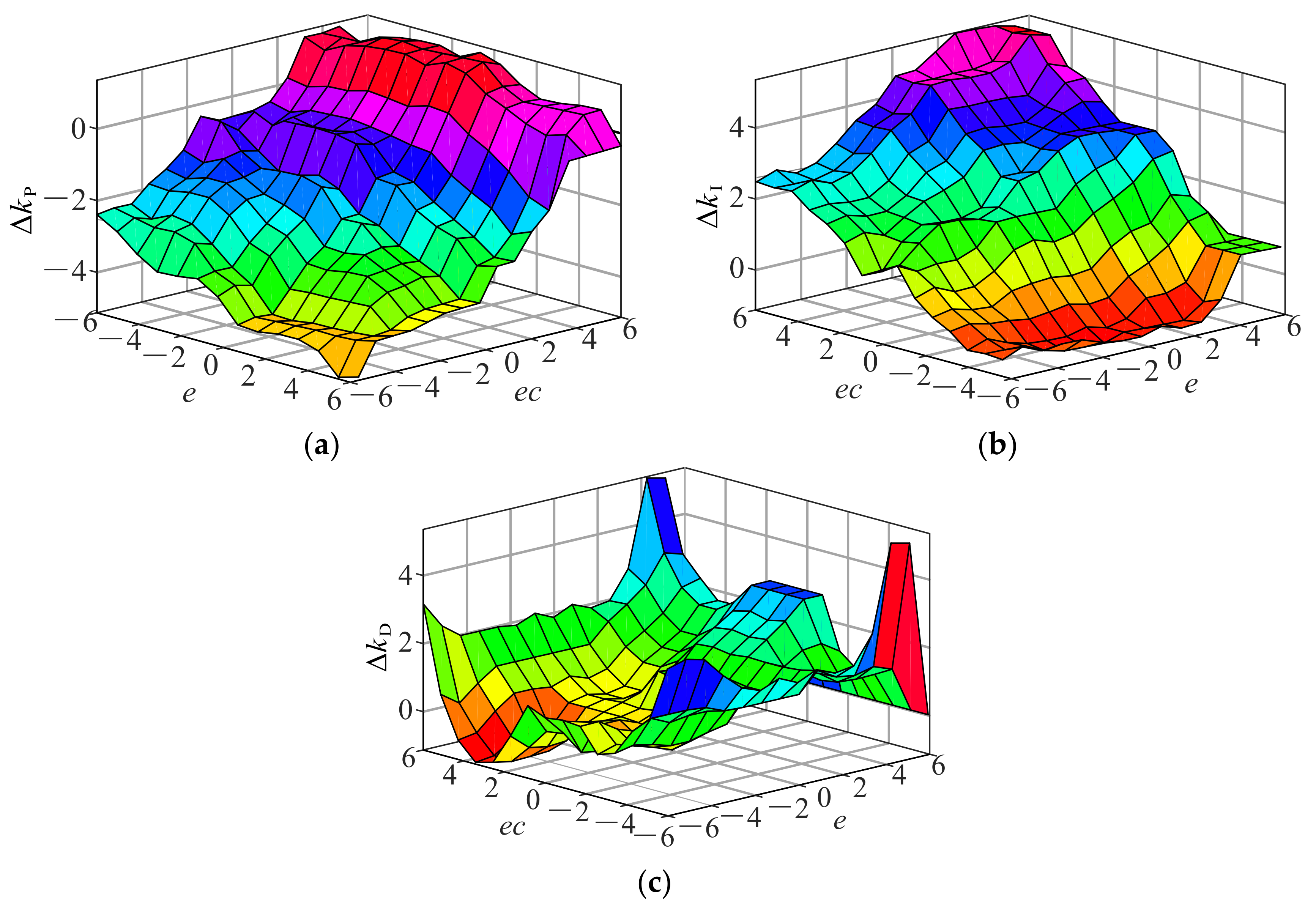
3.3. Fuzzy Adaptive Control Strategy Combined with Pole Assignment

The flexible load will produce lateral vibration in the process of rotation. Lateral vibration will cause elastic deformation of the flexible load. This elastic deformation will affect the output of the servo drive system. In order to improve the stability of the system and reduce the rotation speed fluctuation and output displacement error, this paper adopts a fuzzy adaptive tuning PID control strategy based on pole assignment. This control strategy can track and adjust the PID parameters of the system in real time. Firstly, the traditional parameters of PID controllers are determined by the Ziegler–Nichols method. Then, the pole assignment method with the same real part is used to improve the traditional PI parameter. The approximate range of parameters is optimized and the overshoot of the system is reduced. Finally, the fuzzy control rules of the system are formulated. Based on the PI parameters adjusted by the same real-part pole assignment method, the PID controller parameters are improved. Through the fuzzy rules, the PID parameters of the controller are dynamically adjusted online in real time. Moreover, the input of the flexible-load servo system is compensated adaptively by the feedback mechanism.

When designing the fuzzy adaptive controller, the speed error e and the error change rate ec of the flexible load motor side are taken as the input variables. Then, the fuzzy results $\Delta k_{\mathrm{P}}$, $\Delta k_{\mathrm{I}}$, and $\Delta k_{\mathrm{D}}$ are obtained as output variables after fuzzy reasoning through fuzzy rules. Finally, $\Delta k_{\mathrm{P}}$, $\Delta k_{\mathrm{I}}$, and $\Delta k_{\mathrm{D}}$ are used to adjust the improved PID control parameters, as shown in Equation (55) below, and the exact results of the output variables are obtained by defuzzification. Thus, the control block diagram of the flexible-load servo system is shown in Figure 4.

$$\{\begin{array}{c}{k}_{\mathrm{P}}=k_{\mathrm{P}}^{\prime }+\Delta k_{\mathrm{P}}\\ k_{\mathrm{I}}=k_{\mathrm{I}}^{\prime }+\Delta k_{\mathrm{I}} ,\\ k_{\mathrm{D}}=k_{\mathrm{D}0}^{\prime }+\Delta k_{\mathrm{D}}\end{array}$$

(55)

where $k_{\mathrm{P}}^{\prime }$ and $k_{\mathrm{I}}^{\prime }$ are the parameters improved by using the same real-part pole assignment method, and $k_{\mathrm{D}0}^{\prime }$ is the traditional controller parameters obtained by the Ziegler–Nichols method.

The fuzzy adaptive tuning PID controller used in this paper is a two input and three output controller, where the input variables are e and ec, and the output variables are $\Delta k_{\mathrm{P}}$, $\Delta k_{\mathrm{I}}$, and $\Delta k_{\mathrm{D}}$. The fuzzy domain of the input and output variables of the fuzzy controller is set as [–6, 6], the input error domain is set as [−0.1, 0.1], the error change rate domain is set as [−0.3, 0.3], and the actual output controller domain is set as [−0.6, 0.6]. However, in the design of a fuzzy controller, these five parameters cannot be directly identified, so these five parameters should be fuzzified, as shown in Equation (56):

$$e, ec, \Delta k_{\mathrm{P}}, \Delta k_{\mathrm{I}}, \Delta k_{\mathrm{D}}=\left[\begin{array}{ccc}\mathrm{NB}& \mathrm{NM}& \mathrm{NS}\end{array}\begin{array}{ccc}\mathrm{ZO}& \mathrm{PS}& \begin{array}{cc}\mathrm{PM}& \mathrm{PB}\end{array}\end{array}\right],$$

(56)

P stands for positive definite and N for negative definite. B, M, and S are large, medium, and small, respectively. In particular, ZO stands for zero.

In this paper, the Gaussian function is chosen as the membership function of the input and output of the fuzzy controller. The number of fuzzy sets for each input variable is seven, and there are two input variables. Therefore, 49 fuzzy rules correspond to output variables and can be obtained. Thus, the fuzzy rule inference relation diagram can be designed, as shown in Figure 5. The fuzzy control rules of output variables are shown in

Table 2. Fuzzy rule control table of $\Delta k_{\mathrm{P}}$.

ec/e	PB	PM	PS	ZO	NS	NM	NB
PB	NB	NB	NM	NM	NM	ZO	ZO
PM	PB	ZO	PM	PM	ZO	ZO	NS
PS	PB	PM	PM	PM	PS	PS	NS
ZO	NM	NM	NS	ZO	PS	PS	PM
NS	NS	NS	ZO	PS	PS	PM	PM
NM	NS	ZO	PS	PS	PM	PB	PB
NB	ZO	ZO	PS	PM	PM	PB	PB

,

Table 3. Fuzzy rule control table of $\Delta k_{\mathrm{I}}$.

ec/e	PB	PM	PS	ZO	NS	NM	NB
PB	PB	PB	PM	PS	PS	ZO	ZO
PM	PB	PB	PM	PM	PS	ZO	ZO
PS	PB	PM	PS	PS	ZO	NS	NM
ZO	PM	PS	NS	PS	PS	ZO	ZO
NS	PM	PS	PS	ZO	PS	ZO	ZO
NM	ZO	ZO	NS	NS	NM	NB	NB
NB	ZO	NS	NS	NM	NM	NB	NB

and

Table 4. Fuzzy rule control table of $\Delta k_{\mathrm{D}}$.

ec/e	PB	PM	PS	ZO	NS	NM	NB
PB	PB	PS	PS	PS	PM	PB	PB
PM	PB	PB	PS	PS	PM	PM	PB
PS	ZO	ZO	NS	NS	ZO	ZO	ZO
ZO	ZO	NS	NS	ZO	NS	NS	ZO
NS	ZO	NS	NS	NS	NM	NM	ZO
NM	ZO	NS	NS	NM	NB	NS	PS
NB	PS	NM	NB	NB	NB	NS	PS

.

4. Numerical Simulation Analysis of the System

For the flexible-load servo drive system, the fuzzy adaptive control method combined with pole assignment is used to adjust the controller parameters in real time. In order to study the control characteristics of the system, three different load conditions are selected for numerical simulation. The errors of output angle and output torque under the same working condition are analyzed. The flexible load parameters under three different working conditions are shown in

Table 5. Flexible load parameters in 3 cases.

Determinants	Condition 1	Condition 2	Condition 3
Flexible load length l/m	0.4	0.6	0.8
Flexural stiffness of a flexible load EI/Nm2	400	400	400
Line density of flexible load ρA/kg/m2	5	3.333	2.5
Modal coupling coefficient Fai/kg1/2m	0.455	0.6826	0.9101
Inertia of a flexible load Jl/kgm2	0.1067	0.24	0.427
Modal frequencies of flexible loads ωi/rad/s	196.5294	106.9771	69.4836
Characteristic roots of the mode function β1	1.875	1.875	1.875
Moment of inertia of motor Jm/kgm2	0.36	0.72	1.28
Torsional stiffness ks/Nm/rad	405	405	405

below.

According to the flexible loads under three different conditions in the table, three different control strategies are used, namely, traditional PID, pole assignment method to improve PID, and fuzzy adaptive PID. The sinusoidal function is used as the input signal for numerical simulation, and the simulation results are shown in Figure 6, Figure 7 and Figure 8. Figure 6, Figure 7 and Figure 8 show the speed, angle, elastic deformation, and torque output by the flexible load side of the servo system under three working conditions.

Figure 6a,b show the fluctuations of the system speed and angle, respectively. It can be seen that under the condition of working condition 1, the control strategy of PID is improved by using the traditional PID and pole assignment method alone, and the fluctuation of system output is relatively drastic. When the working time is about 10 s, the system output still has a large fluctuation. Compared with the simulation results, after using the same real-part pole assignment method to improve the PID control strategy, the output fluctuation of the system will be reduced, but the reduction amplitude is not obvious. After the fuzzy adaptive method is used to adjust the PID parameters, the fluctuation amplitude of the system output is obviously reduced, and the stability of the system is improved.

Figure 6c,d show the elastic deformation of the flexible load and the fluctuation of the load end torque. It can be seen that with the extension of working time, using the traditional PID control strategy, the deformation of the flexible load and the load end torque will continue to increase. This can not make the system tend to a stable state, and will eventually lead to the overall system imbalance and the decline of working accuracy. When the pole assignment improved PID control strategy and fuzzy adaptive tuning improved PID control strategy are used, the deformation of the flexible load and the torque fluctuation at the load end decrease steadily. These two methods are effective to improve the stability of the system. By comparing the two effective methods, it can be clearly seen from the figures that the latter has the advantages of faster response speed, smaller volatility, and more stability than the former, and the improvement effect of the system stability is more obvious.

Similarly, as shown in Figure 7 and Figure 8, the output results of working conditions 2 and 3 have the same trend as that of working condition 1. It is shown that the fuzzy adaptive tuning PID control strategy combined with pole assignment has a good effect on the adjustment of the flexible-load servo control system. This control strategy can effectively suppress the system speed and torque fluctuations caused by vibration and reduce the system angle error and the elastic deformation of the load end.

We perform a longitudinal comparison of the output results under three different working conditions. As shown in subfigures (a) and (b) in Figure 6, Figure 7 and Figure 8, under the same load mass, with the increase of the flexible load length, the fluctuations of the system output speed and angle gradually increase. In particular, in subfigures (c) and (d) of Figure 6, Figure 7 and Figure 8, the elastic deformation and output torque of the flexible load increase more obviously.

The output angle error of the flexible-load servo system is obtained after three kinds of control strategies are applied and three kinds of conditions are simulated, respectively. The error distribution is shown in Figure 9. Figure 9a is the absolute error statistical index of the system output angle, and Figure 9b is the variance diagram of the system output angle. It can be seen that in the three working conditions, when the traditional PID control strategy is used, the absolute error value and variance value of the system output angle are the largest when the flexible load length is the longest, and the maximum value is 0.144 and 0.704, respectively. When the fuzzy PID control strategy is adopted and when the flexible load length is the smallest, the absolute error value and variance value of the system output angle are the smallest, which are 0.034 and 0.549, respectively.

As shown in Figure 9a, it can be seen from the high and low trend of the bar chart that under three different circumstances, the absolute error of the system output angle is improved most obviously by the fuzzy adaptive PID control method, and the improvement degree can reach about 10% on average. When the same control method is used to control the flexible-load system under three different working conditions, the comparison shows that the error change rate of the traditional PID control method is the largest, up to about 3%, indicating that this method has poor control over the system output fluctuation. By using the fuzzy adaptive PID control method, the system output angle error can be effectively reduced. This method can reduce the absolute error to about 3.6%, and the error change rate can be reduced to 0.3%. As can be seen from Figure 9b, with the increase of the flexible load length, the variance value of the traditional PID control method fluctuates the most. When the fuzzy adaptive PID control method is used, the variance value of the fuzzy adaptive PID control method is reduced by 10% on average compared with the traditional PID control method, and the system output angle fluctuation is more stable. In summary, the fuzzy adaptive tuning PID control strategy combined with the pole assignment method can significantly reduce the output fluctuation of the system and effectively improve its stability.

5. Conclusions

In this paper, the dynamic modeling of a servo-driven flexible-load system is carried out considering the nonlinear characteristics of the system. Three control strategies of traditional PID, same real-part pole assignment tuning PID, and fuzzy adaptive tuning PID combined with pole assignment are used to control the vibration of the system. The vibration law of flexible load with three different lengths is discussed, and the conclusions are as follows:

(1)

The dynamic modeling of the servo-driven flexible-load system established in this paper takes into account that the flexibility in the load will cause significant fluctuations in the system speed output, which will cause a large deviation in the system angle and displacement output. The unified dynamic model of the system is established.

(2)

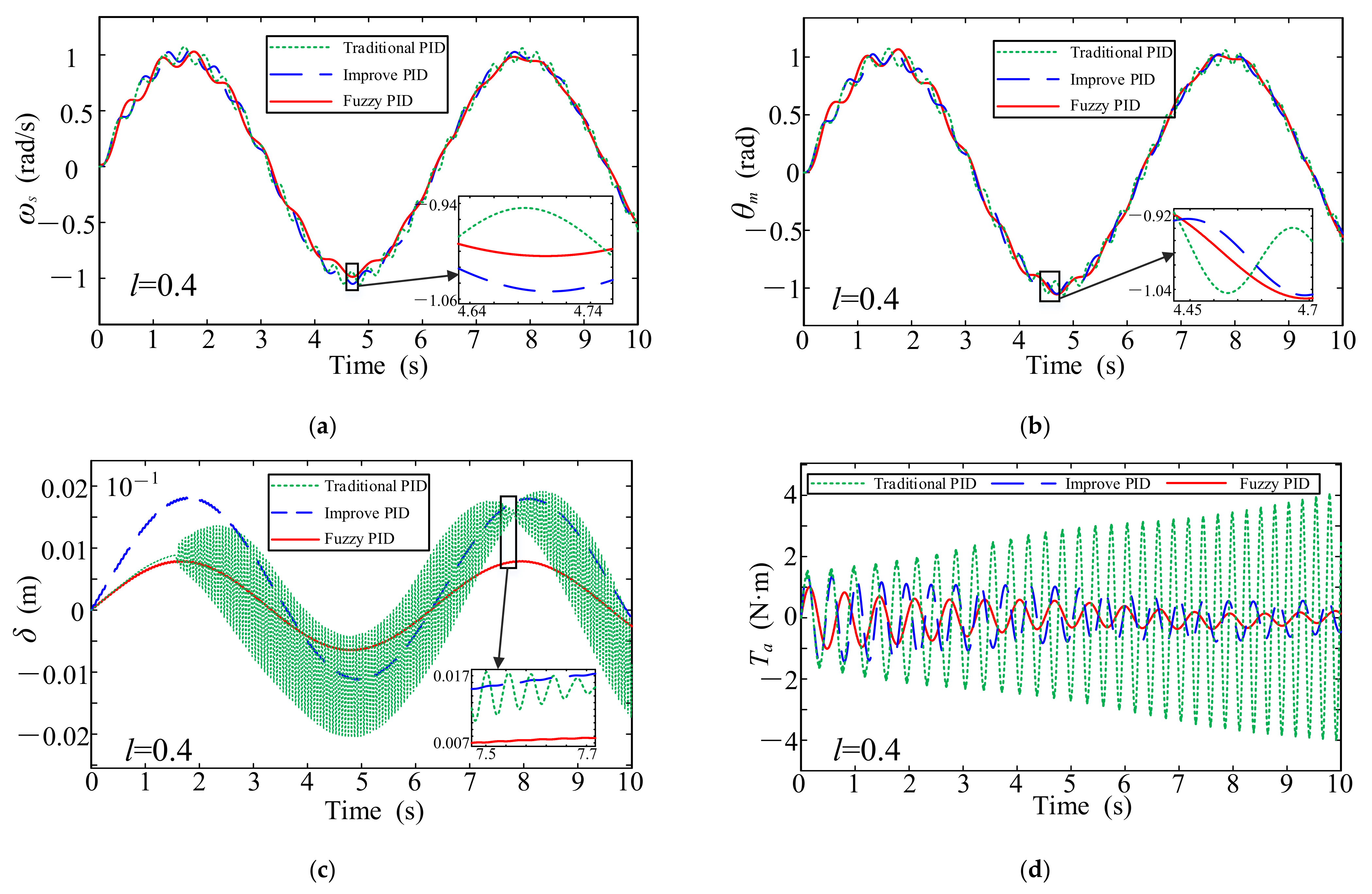
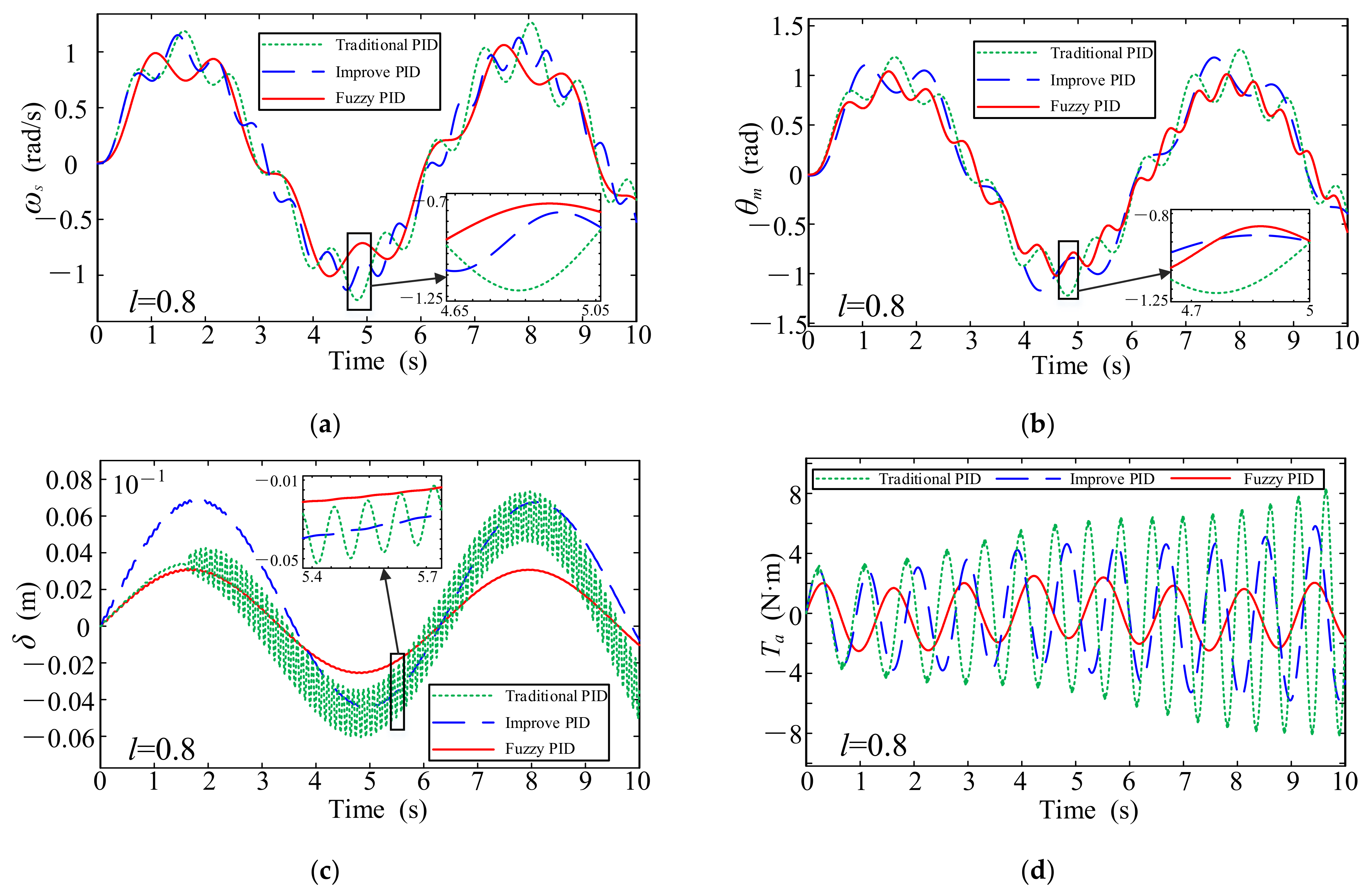
The proposed fuzzy adaptive tuning PID control strategy combined with pole assignment is based on the traditional PID parameters. Firstly, the same real-part pole assignment method is used to adjust PI parameters, and then the fuzzy adaptive control strategy is applied to adjust the adjusted PID parameters to adjust the input variables of the system in real time. The simulation results show that the control strategy is stable and reliable when used to suppress system vibration.

(3)

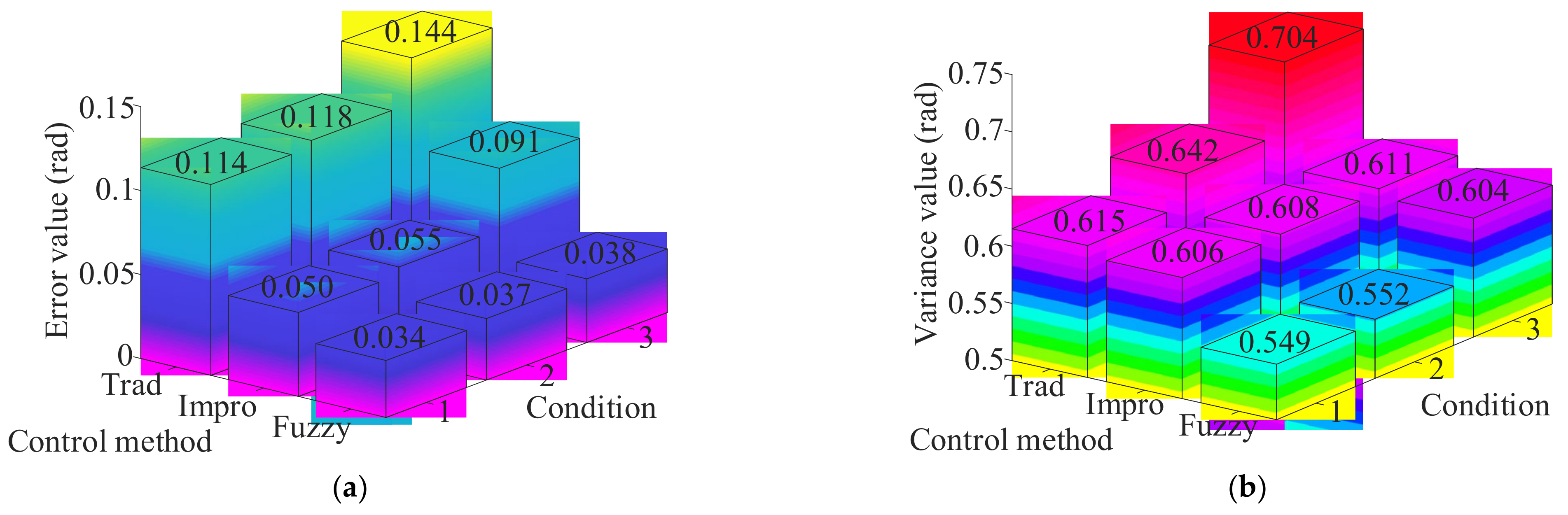
By comparing the system output angle error and flexible load terminal deformation under three different working conditions, it can be seen that the system angle error and flexible load deformation increase with the increase of flexible load length. The control strategy proposed in this paper can reduce the system output angle error and the deformation of the flexible load by 10% on average. From the angle of error analysis, it is proved that the control strategy proposed in this paper can effectively reduce the speed fluctuation of the servo-driven flexible-load system and improve the working accuracy of the system.

Based on the above research contents and conclusions, more nonlinear factors affecting the system stability can be considered for the next research work. At the same time, the direction of the intelligent control algorithm can be improved. It provides theoretical suggestions for future stability research into flexible-load servo systems.

References

1. Wu, J.J.; Zhang, Z.K. An Improved Procedure for Manufacture of 3D Tubes with Springback Concerned in Flexible Bending Process. Chin. J. Aeronaut. 2021, 34, 267–276. [Google Scholar] [CrossRef]
2. He, W.; Meng, T.T.; He, X.Y.; Sun, C.Y. Iterative Learning Control for a Flapping Wing Micro Aerial Vehicle Under Distributed Disturbances. IEEE Trans. Cybern. 2019, 49, 1524–1535. [Google Scholar] [CrossRef] [PubMed]
3. McGarry, L.; Butterfield, J.; Murphy, A. Assessment of ISO Standardisation to Identify an Industrial Robot’s Base Frame. Robot. Comput. Integr. Manuf. 2022, 74, 102275. [Google Scholar] [CrossRef]
4. Stefano, M.D.; Balachandran, R.; Secchi, C. A Passivity-Based Approach for Simulating Satellite Dynamics with Robots: Discrete-Time Integration and Time-Delay Compensation. IEEE Trans. Rob. 2020, 36, 189–203. [Google Scholar] [CrossRef] [Green Version]
5. Efafi, M.; Hosseini, S.A.A.; Tourajizadeh, H. Robust Control and Vibration Reduction of a 3D Nonlinear Flexible Robotic Arm. Iran. J. Sci. Technol. Trans. Mech. Eng. 2022, 144, 1–7. [Google Scholar] [CrossRef]
6. Geng, R.H.; Bian, Y.S.; Zhang, L.; Guo, Y.Z. A Saturation-Based Method for Primary Resonance Control of Flexible Manipulator. Machines 2022, 10, 284. [Google Scholar] [CrossRef]
7. Li, Y.Y.; Ge, S.S.; Wei, Q.P.; Gan, T.; Tao, X.L. An Online Trajectory Planning Method of a Flexible-Link Manipulator Aiming at Vibration Suppression. IEEE Access 2020, 8, 130616–130632. [Google Scholar] [CrossRef]
8. Oh, S.; Kong, K. High-Precision Robust Force Control of a Series Elastic Actuator. IEEE/ASME Trans. Mechatron. 2017, 22, 71–80. [Google Scholar] [CrossRef]
9. Lightcap, C.A.; Banks, S.A. An Extended Kalman Filter for Real-Time Estimation and Control of a Rigid-Link Flexible-Joint Manipulator. IEEE Trans. Control Syst. Technol. 2010, 18, 91–103. [Google Scholar] [CrossRef]
10. Krysko, A.V.; Awrejcewicz, J.; Kutepov, I.E.; Krysko, V.A. Stability of Curvilinear Euler-Bernoulli Beams in Temperature Fields. Int. J. Non-Linear Mech. 2017, 94, 207–215. [Google Scholar] [CrossRef]
11. He, X.Y.; Song, Y.H.; Han, Z.J.; Zhang, S.; Jing, P.; Qi, S.W. Adaptive Inverse Backlash Boundary Vibration Control Design for an Euler–Bernoulli Beam System. J. Frankl. Inst. 2020, 357, 3434–3450. [Google Scholar] [CrossRef]
12. Parviz, H.; Fakoor, M. Free Vibration of a Composite Plate with Spatially Varying Gaussian Properties Under Uncertain Thermal Field Using Assumed Mode Method. Phys. A Stat. Mech. Its Appl. 2020, 559, 125085. [Google Scholar] [CrossRef]
13. Hao, T.; Wang, H.S.; Xu, F.; Wang, J.C.; Miao, Y.Z. Uncalibrated Visual Servoing for a Planar Two Link Rigid-Flexible Manipulator Without Joint-Space-Velocity Measurement. IEEE Trans. Syst. Man Cybern. Syst. 2022, 52, 1935–1947. [Google Scholar] [CrossRef]
14. Sun, C.Y.; Gao, H.J.; He, W.; Yu, Y. Fuzzy Neural Network Control of a Flexible Robotic Manipulator Using Assumed Mode Method. IEEE Trans. Neural Netw. Learn. Syst. 2018, 29, 5214–5227. [Google Scholar] [CrossRef]
15. Ji, H.R.; Li, D.X. A Novel Nonlinear Finite Element Method for Structural Dynamic Modeling of Spacecraft Under Large Deformation. Thin-Walled Struct. 2021, 165, 107926. [Google Scholar] [CrossRef]
16. Grazioso, S.; Di Gironimo, G.; Iglesias, D.; Siciliano, B. Screw-Based Dynamics of a Serial/Parallel Flexible Manipulator for DEMO Blanket Remote Handling. Fusion Eng. Des. 2019, 139, 39–46. [Google Scholar] [CrossRef]
17. Shao, M.Q.; Huang, Y.M.; Silberschmidt, V.V. Alvaro Cunha. Intelligent Manipulator with Flexible Link and Joint: Modeling and Vibration Control. Shock Vib. 2020, 2020, 4671358. [Google Scholar] [CrossRef] [Green Version]
18. Matsuno, F.; Asano, T.; Sakawa, Y. Modeling and Quasi-Static Hybrid Position Force Control of Constrained Planar 2-Link Flexible Manipulators. IEEE Trans. Robot. Autom. 1994, 10, 287–297. [Google Scholar] [CrossRef]
19. Lu, E.; Li, W.; Yang, X.F.; Wang, Y.Q.; Liu, Y.F. Optimal Placement and Active Vibration Control for Piezoelectric Smart Flexible Manipulators Using Modal H-2 Norm. J. Intell. Mater. Syst. Struct. 2018, 29, 2333–2343. [Google Scholar] [CrossRef]
20. Wang, J.F.; Cao, F.F.; Liu, J.K. Nonlinear Partial Differential Equation Modeling and Adaptive Fault-Tolerant Vibration Control of Flexible Rotatable Manipulator in Three-Dimensional Space. Int. J. Adapt. Control Signal Process. 2021, 35, 2138–2154. [Google Scholar] [CrossRef]
21. Tang, L.W.; Gouttefarde, M.; Sun, H.N.; Yin, L.R.; Zhou, C.J. Dynamic Modelling and Vibration Suppression of a Single-Link Flexible Manipulator with Two Cables. Mech. Mach. Theory 2021, 162, 104347. [Google Scholar] [CrossRef]
22. Chu, M.; Zhang, Y.H.; Chen, G.; Sun, H.X. Effects of Joint Controller on Analytical Modal Analysis of Rotational Flexible Manipulator. Chin. J. Mech. Eng. 2015, 28, 460–469. [Google Scholar] [CrossRef]
23. Shang, D.Y.; Li, X.P.; Yin, M.; Li, F.J. Control Method of Flexible Manipulator Servo System Based on a Combination of RBF Neural Network and Pole Placement Strategy. Mathematics 2021, 9, 896. [Google Scholar] [CrossRef]
24. Shang, D.Y.; Li, X.P.; Yin, M.; Li, F.J. Speed Control Method for Dual-Flexible Manipulator with a Telescopic Arm Considering Bearing Friction Based on Adaptive PI Controller with DOB. Alex. Eng. J. 2022, 61, 4741–4756. [Google Scholar] [CrossRef]
25. Kim, S.M.; Kim, H.; Boo, K.; Brennan, M.J. Demonstration of Non-Collocated Vibration Control of a Flexible Manipulator Using Electrical Dynamic Absorbers. Smart Mater. Struct. 2013, 22, 127001. [Google Scholar] [CrossRef]
26. Wu, Q.C.; Wang, X.S.; Chen, B.; Wu, H.T.; Shao, Z.Y. Development and Hybrid Force/Position Control of a Compliant Rescue Manipulator. Mechatronics 2017, 46, 143–153. [Google Scholar] [CrossRef]
27. Dindorf, R.; Wos, P. A Case Study of a Hydraulic Servo Drive Flexibly Connected to a Boom Manipulator Excited by the Cyclic Impact Force Generated by a Hydraulic Rock Breaker. IEEE Access 2022, 10, 7734–7752. [Google Scholar] [CrossRef]
28. Ding, Y.S.; Xiao, X.; Huang, X.R.; Sun, J.X. System Identification and a Model-Based Control Strategy of Motor Driven System with High Order Flexible Manipulator. Ind. Robot 2019, 46, 672–681. [Google Scholar] [CrossRef]
29. Li, X.P.; Shang, D.Y.; Li, H.Y.; Li, F.J. Resonant Suppression Method Based on PI control for Serial Manipulator Servo Drive System. Sci. Prog. 2020, 103, 36850420950130. [Google Scholar] [CrossRef]
30. Gao, H.J.; He, W.; Song, Y.H.; Zhang, S.; Sun, C.Y. Modeling and Neural Network Control of a Flexible Beam with Unknown Spatiotemporally Varying Disturbance Using Assumed Mode Method. Neurocomputing 2018, 314, 458–467. [Google Scholar] [CrossRef]
31. Wang, H.P.; Zhou, X.Y.; Tian, Y. Robust Adaptive Fault-Tolerant Control Using RBF-Based Neural Network for a Rigid-Flexible Robotic System with Unknown Control Direction. Int. J. Robust Nonlinear Control 2022, 32, 1272–1302. [Google Scholar] [CrossRef]
32. Ma, H.; Zhou, Q.; Li, H.Y.; Lu, R.Q. Adaptive Prescribed Performance Control of A Flexible-Joint Robotic Manipulator With Dynamic Uncertainties. IEEE Trans. Cybern. 2021, 3091531, 1–11. [Google Scholar] [CrossRef]
Figure 1. Schematic diagram of flexible load: (a) 3D model diagram; (b) schematic diagram of an equivalent flexible connecting rod.
Mathematics 10 03962 g001
Figure 2. Standard form block diagram of speed loop of a traditional PI control system.
Mathematics 10 03962 g002
Figure 3. Zero pole distribution diagram of the same real-part pole assignment method.
Mathematics 10 03962 g003
Figure 4. Control block diagram of a flexible-load servo system. (a) Block diagram of traditional PID control method. (b) Block diagram of pole assignment improved PID control method. (c) Block diagram of fuzzy adaptive PID control method.
Mathematics 10 03962 g004
Figure 5. Fuzzy rule inference relation diagram of Δ k P , Δ k I , and Δ k D . (a) Fuzzy rule inference relation diagram of Δ k P . (b) Fuzzy rule inference relation diagram of Δ k I . (c) Fuzzy rule inference relation diagram of Δ k D .
Mathematics 10 03962 g005
Figure 6. The output curve of the flexible load side in case 1: (a) the output speed; (b) the output angle; (c) output elastic deformation; (d) the output torque.
Mathematics 10 03962 g006
Figure 7. The output curve of the flexible load side in case 2: (a) the output speed; (b) the output angle; (c) output elastic deformation; (d) the output torque.
Mathematics 10 03962 g007
Figure 8. The output curve of the flexible load side in case 3: (a) the output speed; (b) the output angle; (c) output elastic deformation; (d) the output torque.
Mathematics 10 03962 g008
Figure 9. Error statistical index: (a) absolute error statistics index; (b) statistical index of variance.
Mathematics 10 03962 g009