Cross Domain Data Generation for Smart Building Fault Detection and Diagnosis

Abstract

Benefiting extensively from the Internet of Things (IoT) and sensor network technologies, the modern smart building achieves thermal comfort. It prevents energy wastage by performing automatic Fault Detection and Diagnosis (FDD) to maintain the good condition of its air-conditioning systems. Often, real-time multi-sensor measurements are collected, and supervised learning algorithms are adopted to exploit the data for an effective FDD. A key issue with the supervised methods is their dependence on well-labeled fault data, which is difficult to obtain in many real-world scenarios despite the abundance of unlabelled sensor data. Intuitively, the problem can be greatly alleviated if some well-labeled fault data collected under a particular setting can be re-used and transferred to other cases where labeled fault data is challenging or costly. Bearing this idea, we proposed a novel Adversarial Cross domain Data Generation (ACDG) framework to impute missing fault data for building fault detection and diagnosis where labeled data is costly. Unlike traditional Transfer Learning (TL)-related applications that adapt models or features learned in the source domain to the target domain, ACDG essentially “generates” the unknown sensor data for the target setting (target domain). This is accomplished by capturing the data patterns and common knowledge from known counterparts in the other setting (source domain), the inter-domain knowledge, and the intra-domain relations. The proposed ACDG framework is tested with the real-world Air Handling Unit (AHU) fault dataset of the ASHRAE Research Project 1312. Extensive experimental results on the cross-domain AHU fault data showed the effectiveness of ACDG in supplementing the data for a missing fault category by exploiting the underlying commonalities between different domain settings.

1. Introduction

Enabled by the advent of IoT, a smart city for the future will be able to address multiple areas of citizens’ daily life, such as transportation, energy, healthcare, building, and public safety, in an intelligent, energy-efficient, and cost-effective way [1]. Within this scope, smart buildings, shown in the lower part of Figure 1, constitute a key component of a smart city plainly because a major part of citizens’ daily routines is performed within the indoor environment. Moreover, buildings currently consume more than 40% of the total world’s energy. A large proportion of such energy usage, unfortunately, is wasted due to miscellaneous faults, namely, poor maintenance, degradation, and improperly controlled equipment and appliances particularly related to the Heating, Ventilation, and Air-Conditioning (HVAC) systems [2]. As such, an indispensable underpinning for modern smart buildings is the realization of automatic and data-driven Fault Detection and Diagnosis (FDD), via various data collected from the sensor networks.

Faults in smart buildings are usually gradual deficiencies in the HVAC systems which cause performance degradation. In contrast, the system still functions to a certain extent, and faults are hard to manually notice until abrupt system malfunctioning has been witnessed [3]. To identify faults before heavy economic losses are generated, FDD strategies should be carefully designed with capabilities to monitor the inner connections among different HVAC components [4]. Driven by the superiority in revealing the underlying patterns and correlations among features over traditional model-based methods, a wide range of supervised pattern classification techniques have been explored in the building FDD field. To list a few, existing literature includes multivariate regression models [5], Bayes classifiers [6], neural networks (NN) [7,8], linear discriminant analysis (LDA) [3], Gaussian mixture models [9], support vector machines (SVM) [10,11], and tree-structured learning method [12,13]. However, supervised data-driven FDD methods have limited usefulness in practice due to the following factors:

• Lack of real-life labeled fault data: Most well-labeled fault datasets are collected from experiments conducted in laboratory test beds or synthetic systems. Labeled fault data in real-life smart building systems are rare—the raw sensor measurements are typically unlabelled [14].
• Limited transferability of labeled fault data: The existing well-labeled fault datasets should not be directly applied to similar smart building systems as the environmental factors and equipment settings can be different from the laboratory test-beds or synthetic smart building systems and are constantly changing (e.g., due to seasonal changes) [15].

This paper deals with the limitations above, particularly for smart building systems, but the framework proposed can be readily applied to many other scenarios involving FDD for IoT. Traditionally, to tackle the issue that sensor measurements cannot be directly re-used or transferred, expert rules (Usually, these rules are upper and lower bounds (thresholds) of one or several variables.) are encoded by researchers and building experts on the basis of field tests in different buildings [16,17]. They are then deployed as standard regulations to detect typical faults in commercial buildings. Although rule-based FDD is intuitive and widely applicable in existing HVAC systems, the high false alarm rate and/or the low sensitivity are obvious defections since few hidden correlations and patterns cannot be summarized or presented by the bound-like rules.

In recent years, researchers have been exploring statistical tools, and machine learning (more recently, deep learning) techniques to address the scarcity of well-labeled data and the synthetic data generation problem. Within the framework of statistical learning, Bootstrap [18], and Jackknife [19] are two popular re-sampling methods addressing the data limitation issue. By iteratively re-sampling a dataset with replacement, the dataset can be enlarged while maintaining the underlying distributions. However, the re-sampled dataset is not very helpful in establishing a better FDD model since the data distribution is not transformed or enhanced into a better embedding simply by the repeated re-sampling procedures. Instead, the recently proposed Generative Adversarial Networks (GAN) [20] learns the underlying data distribution or embedding more smartly: the GAN framework allows a generator to be adversarially and simultaneously trained together with a binary classifier, thereby enabling the generator to capture the implicit distribution of the training samples more effectively. Although GAN can generate “realistic” samples that better reflect intrinsic patterns, their distribution aligns strictly with the training data. In other words, standard GAN generation cannot generate data for another domain with a different distribution from the training domain.

To enable the utilization of knowledge learned from the source domain to a target domain, a resort to Transfer Learning (TL) or cross-domain machine learning [21,22] seems necessary. As shown in Figure 1, challenges for solving the problem of limited labeled data by a TL-based sensor data generation are two-fold: (1) it is hard to capture the hidden knowledge from the source domain that can optimally benefit the target learning task and (2), it is hard to generate new distributions in a new domain without known labeled samples. In previous work, such as in [23,24], an intuitive idea was adapting data in both domains into a common inter-space. To achieve this, a few shots of data in the target domain should be at least available for the distribution alignment. However, given a target domain with a missing category, it is hard to adapt the learned classifier because no anchors are available to measure the distribution shift or to capture the hidden information from the target domain. In [4,25], authors transferred the knowledge between data and fault attributes to diagnose unknown faults with zero training samples. This method is novel and effective, but well-summarized expert knowledge is required and essential, and the unknown faults should be in the same domain as the known faults.

To address these challenges and provide a handy solution to label scarcity, we need to generate data samples in the target domain with relevant patterns that are useful for the target learning task (For the FDD problem at hand, the learning task is imbalanced classification). To this end, it will be necessary to capture the intrinsic embedding between the data in the source and target domains such that the source domain data distribution can be effectively adapted and transformed for the data generated in the target domain. Thus, a novel procedure for data generation, namely the Adversarial Cross domain Data Generation (ACDG) framework, was proposed to exploit the labeled fault data collected for known faults in both domains to generate the data for a missing fault in one domain for FDD applications (As will be mentioned in Section 4.2, AHU working condition is largely dependent on the seasonal environmental factors. Thus, the same faults in different seasons can be viewed as data in two domains).

In contrast with the previous works, the key contributions of this work are as follows:

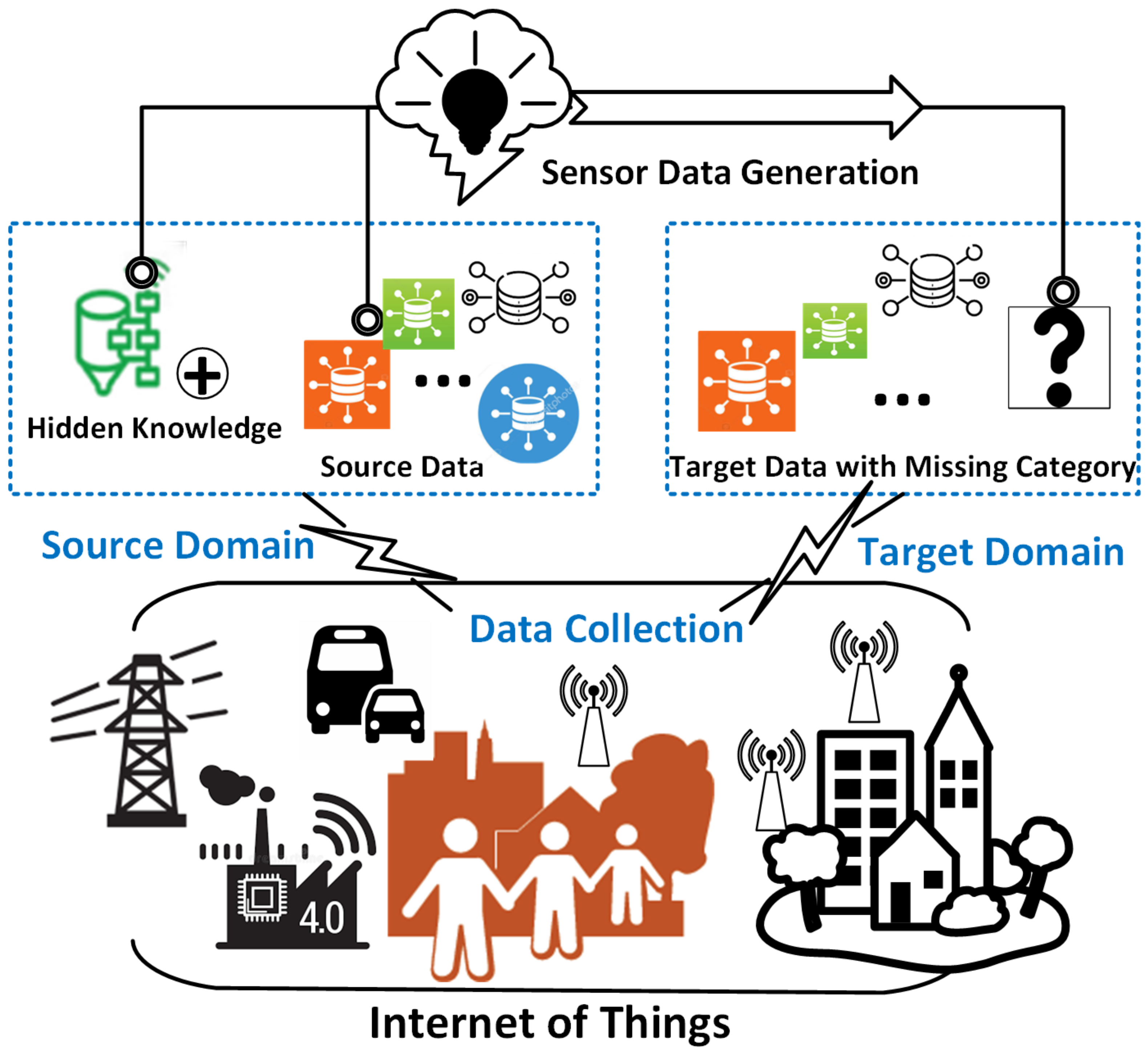
• A ACDG framework was proposed to generate unknown target faults based on known faults for the learning task in a target setting.
• Unlike existing TL-based FDD work, the proposed ACDG framework captured both the inter-domain knowledge and the intra-domain class relations.
• With experiments on the ASHRAE RP-1312 dataset, the proposed ACDG framework was proven to generate building faults in one season based on their counterparts in other seasons.
• While this paper has focused on building fault generation, the proposed ACDG framework is general and should also apply to other sensor data generation applications.

The remaining part of this paper is organized as follows. Section 2 introduces related works. Section 3 shows the framework of ACDG and its mathematical formulation. The building mechanical system is introduced in Section 4. Next, experiments with real data and experimental results are presented in Section 5. Finally, Section 6 summarizes the paper and suggests possible future work.

2. Related Works

The proposed ACDG framework is grounded on the machine learning areas of Generative Adversarial Networks and transfer learning and advances both methods to achieve cross-domain data generation. The following subsections discuss their relations and the technical novelty of the proposed method.

2.1. Generative Adversarial Networks

The recent GAN framework enables researchers to build a generative model via adversarial learning [20]. GAN’s training process corresponds to a minimax two-player game where two deep networks are trained via an adversarial manner: simultaneously training a generative network to capture the data distribution and a discriminating network to distinguish whether a sample comes from the training data set or the generator. During the past years, GAN has achieved promising success in generating realistic-looking images [26,27]. Researchers have attempted to adopt the GAN framework for generating other data types, such as sequential data and time series after that. For example, it has been used to produce polyphonic music with recurrent neural networks implemented as its generator and discriminator [28], and to generate real-valued medical time series with a conditional version of recurrent GAN [29]. These existing successes of GAN in generating complex datasets are highly supportive of using GAN for realistic-looking data generation. In [30], authors proposed a Disco-GAN framework to learn the cross-domain relation to generating images in the target domain, which is a meaningful attempt to apply GANs for unknown data generation via cross-domain knowledge transfer. However, the intra-domain class relation is not considered.

2.2. Transfer Learning

A common assumption for many machine learning and data mining algorithms is that the training and testing data must be in the same feature space having the same distribution. However, this assumption is easily violated in many real applications [31]. In such cases, transfer learning from source to target would fulfill the classification task in the target domain by transferring the knowledge learned in the source domain without the expense of re-collecting labeled data [22]. As a summary, existing transfer learning methods can be summarized into the following four categories:

• Instance-based Transfer: It is intuitively assumed that certain parts of the data in the source domain can be reused for learning in the target domain by re-weighting [32,33]. These approaches can be viewed as an improvement of the semi-supervised learning method by using unlabelled data to transfer data (either through re-weighting or projection) from the source domain to the target domain. In contrast, little hidden knowledge about the data and system structure is revealed and conveyed.
• Feather Representation Transfer: In this case, transfer learning is enhanced from the previous case where unlabelled data is applied directly by digging “robust” features in the source domain and then transferring them to help with the target task [34,35]. By projecting the features learned in the source domain to the target domain with a new representation, the performance of the target can be somewhat improved. However, the knowledge conveyed by feature transfer is limited due to information loss during projection.
• Parameter Transfer: Assuming that the source tasks and the target tasks share some parameters or prior distributions of the hyper-parameters of the models [36,37], this kind of transfer learning tries to discover the shared parameters or priors from the source domain and then share them, e.g., through Bayesian priors, across different domains. Although effective, this kind of transfer strongly requires the two domains to share similar distributions. Otherwise, the shared parameters would not be much helpful.
• Knowledge Transfer: The aforementioned transfer learning methods all attempt to unify the data distributions in source and target domains by projection or alignment. In these cases, intrinsic patterns in the source data may not be fully uncovered as the relational knowledge between two domains is not comprehensively considered. Researchers proposed to learn the data relationship between two domains with models capable of learning representations, e.g., deep neural networks [38]. The learned embedding of hidden data patterns between different domains is a key factor in this kind of transfer learning and thus results in a well-known sub-filed called domain adaptation [39,40].

In this work, GAN’s generation function was integrated with cross-domain knowledge transfer to generate unknown fault data in the target domain based on its counterpart in the source domain by capturing both the inter-domain knowledge and the intra-domain class associations.

3. Adversarial Cross Domain Data Generation Framework

3.1. Problem Statement

Supervised fault detection and diagnosis for building systems are defined as follows: given a set of sensor measurements, the task is to annotate it with labels to describe the system’s working conditions (normal or abnormal with certain faults). In other words, the FDD problem is a prediction task with the primary goal to learn a function $f:\mathcal{X}\to \mathcal{Y}$ based on the n-class labelled training dataset $\mathcal{S}=\{(x_i,y_i),i=1,2,\dots ,n\}$. Often with certain constraints on its complexity for regularization, the function maps an input $x_i$ in the space of measurements $\mathcal{X}$ to an output $y_i$ in the space of training labels $\mathcal{Y}$. Labeled pairs $(x_i,y_i)$ for each class should be included in the training dataset.

The application case for this work is to generate data samples for one domain that does not have the corresponding labeled fault data points by transferring and leveraging hidden knowledge and correlations from its counterpart in another domain. More specifically, as shown in the lower part of Figure 2, the task is to build a generator $G^{ST}:{\mathcal{X}}^S\to {\mathcal{X}}^{ST}$ to map data samples $(x_{n+1}^S,y_{n+1}^S)$ from a source domain to a set of new samples for the target domain, denoted by $(x_{n+1}^{ST},y_{n+1}^{ST})$. Then, the FDD task is to learn a mapping function $f^{\prime }:{\mathcal{X}}^{\prime }\to {\mathcal{Y}}^{\prime }$ based on the extended training dataset ${\mathcal{S}}^{\prime }=\{(x_i,y_i)\cup (x_{n+1}^{ST},y_{n+1}^{ST})$, $i=1,2,\dots ,n\}$. The benefit of directly generating extended data samples, versus implicitly extrapolating some functional form, lies in its flexibility to accommodate various tasks and capacity to cover complex relational transfers via a simple data distribution.

Within this work, different seasonal conditions are used as concrete examples for different domains (source and target). With a slight abuse of notation, the terms’ label, category, and fault are noted interchangeably - they all stand for different fault types in the datasets. Among them, the normal condition is treated as one category of FDD for simplicity.

3.2. Architecture

The proposed ACDG architecture can be summarized into three two-model-training processes and one data-generation process, as shown in Figure 2. Firstly, in the Source-to-Target training process, the labelled fault data sets ($F_i^S,i=1,2,3,4$) are fed into the “source-to-target generator” ($G^{ST}$) to generate $F_i^{ST},i=1,2,3,4$. To control the model complexity and encourage the learning of common embedding, the structure of the Encoder-Decoder is imposed to be the same for all the generators in the ACDG network. Similar to the standard GAN process, a discriminator $D^T$ is applied to discriminate the generated data sets ($F_i^{ST},i=1,2,3,4$) and the known faults ($F_i^T,i=1,2,3$) in the target domain. Two efforts are devoted to refining the generation results. On the one hand, a classifier $C^T$ in the target domain is applied to ensure that the generated data sets are correctly categorized. On the other hand, an inverse mapping $G^{TS}$ is also defined to recover the target counterparts from the target domain to the source domain. The recovered faults ($F_i^{STS},i=1,2,3,4$) are enforced to have similar distributions with source faults ($F_i^S,i=1,2,3,4$), respectively. In this way, a classifier $C^S$ trained with the known labeled categorized fault data sets in the source domain would thus be able to classify the recovered data with minimal classification errors.

Simultaneously, to further enhance the learning of cross-domain relationships, the aforementioned training process was also implemented in reverse order. As illustrated in the middle part of Figure 2, during the Target-to-Source process, the known fault data sets ($F_i^T,i=1,2,3$) from the target domain are fed into the generator $G^{TS}$ to generate their counterparts ($F_i^{TS},i=1,2,3$) in the source domain, where they are discriminated by $D^S$ from the known source faults ($F_i^S,i=1,2,3,4$) and should also be recognized by the source domain classifier $C^S$. As before, the recovered $G^{ST}$, $F_i^{TST},i=1,2,3$ should also be distinguishable by the classifier $C^T$ in the target domain with minimal classification error.

In summary, the two sets of generators ($G^{ST}$ and $G^{TS}$) and discriminators ($D^S$ and $D^T$) during the training processes are two coupled GAN models. With a sufficient number of rounds of training, the generator $G^{ST}$ can then be used to generate a set of fault data based on its counterpart in another season (source domain), as shown in the lower part of Figure 2. Since the training process is bi-directional, $G^{TS}$ can also be used to generate fault data based on its counterpart in the target domain. In other words, the source, and target definitions are not fixed in the proposed ACDG framework, allowing each generator to learn a mapping from its input to the output domain and mutually uncover the hidden cross-domain associations in both directions.

3.3. Methodology

Originally, a standard GAN takes random Gaussian noise $Z=\{z_i,i=1,2,\dots ,m\}$, which is a set of multivariate samples taken from a measurable space, as the input and encodes it into hidden features h and generates samples that are similar to realistic samples $X=\{x_i,i=1,2,\dots ,m\}\subseteq {\mathcal{R}}^{M\times T}$, where m is the number of samples. By feeding X and Z to the GAN model, the generator and discriminator are trained with the following two-player minimax game:

$$\begin{array}{c}\underset{G}{min}\underset{D}{max}V(D,G)={\mathcal{E}}_{x\sim p_{data}(X)}\left[logD\left(x\right)\right]\hfill \\ +{\mathcal{E}}_{z\sim p_z(Z)}\left[log(1-D(G\left(z\right)\left)\right)\right]\hfill \end{array}$$

(1)

The proposed ACDG improves the generation task with a key modification—Using samples in one domain as input instead of random noise to generate samples in another domain, i.e., the generator is indeed an Encoder-Decoder by intuition. Denoting the known samples from the source and target by $X^S$ and $X^T$, respectively, one can obtain the following generation results by generating samples in the target domain from the source domain:

$$X^{ST}=G^{ST}\left(X^S\right)$$

(2)

$$X^{STS}=G^{TS}\left(X^{ST}\right)$$

(3)

Subsequently, the minimax function of the GAN model from source to target is modified as follows:

$$\begin{array}{c}\underset{G^{ST}}{min}\underset{D^T}{max}V(D^T,G^{ST})={\mathcal{E}}_{x\sim p_{data}(X^T)}\left[log{D}^T\left(x\right)\right]\hfill \\ +{\mathcal{E}}_{x\sim p_{data}(X^S)}\left[log(1-D^T\left(G^{ST}\left(X^S\right)\right))\right]\hfill \end{array}$$

(4)

Similarly, the generation process and the minimax function for the GAN model from target to source are:

$$X^{TS}=G^{TS}\left(X^T\right)$$

(5)

$$X^{TST}=G^{ST}\left(X^{TS}\right)$$

(6)

$$\begin{array}{c}\underset{G^{TS}}{min}\underset{D^S}{max}V(D^S,G^{TS})={\mathcal{E}}_{x\sim p_{data}(X^S)}\left[log{D}^S\left(x\right)\right]\hfill \\ +{\mathcal{E}}_{x\sim p_{data}(X^T)}\left[log(1-D^S\left(G^{TS}\left(X^T\right)\right))\right]\hfill \end{array}$$

(7)

3.4. ACDG Losses

As is illustrated in Figure 2, four loss functions exist for each GAN model, namely, the G loss ($L_G$) and D loss ($L_D$) extracted from standard GAN framework, and the transfer loss ($L_{TRS}$) and the reconstruction loss ($L_{REC}$) defined in our ACDG framework. Taking the adversarial generation process from source to target for an example, the discriminator $D^T$ in the target domain is trained to minimize the average cross entropy between predicted labels and ground truth, i.e., training D to mark training samples as real and generated samples as false. Thus, the discrimination loss is

$$\begin{array}{c}{L}_{D^T}=\frac{1}{m}\sum _{i=1}^m\left[log{D}^T\left(x_i^T\right)+log(1-D^T\left(G^{ST}\left(x_i^S\right)\right))\right]\hfill \\ \iff min\frac{1}{m}\sum _{i=1}^m\left[-log{D}^T\left(x_i^T\right)-log(1-D^T\left(G^{ST}\left(x_i^S\right)\right))\right]\hfill \end{array}$$

(8)

where $x_i^T,i=1,\dots ,m$ is the target training samples which should be identified as real, and $G^{ST}\left(x_i^S\right),i=1,\dots ,m$ is the generated samples (from source to target) that should be identified as false. Simultaneously, the generator $G^{ST}$ is trained to fool the discriminator so that it would identify as many fake samples as “real” as possible. Specifically, the generation loss is

$$\begin{array}{c}{L}_{G^{ST}}=\sum _{i=1}^{m}log(1-D^T\left(G^{ST}\left(x_i^S\right)\right))\hfill \\ \iff min\sum _{i=1}^{m}log(-D^T\left(G^{ST}\left(x_i^S\right)\right))\hfill \end{array}$$

(9)

As mentioned in Section 3.3, two extra classification losses are defined to measure the performance of the generator in terms of successfully transferred type information and the reconstruction quality of samples after two rounds of generations. Accordingly, the classification losses are included to consolidate the transfer-and-reconstruction and identify categories of generated data.

$$\begin{array}{c}{L}_{TRS}^{ST}=d(X^{ST},X^T)=\frac{1}{n}\sum _{i=1}^n{(y_i^T-\widehat{y^T})}^2\hfill \\ L_{REC}^{TS}=d(X^{STS},X^S)=\frac{1}{n}\sum _{i=1}^n{(y_i^S-\widehat{y^S})}^2\hfill \end{array}$$

(10)

where n is the number of classes in the source domain.

Similarly, loss functions for the adversarial generation process from target to source are as follows:

$$\begin{array}{c}{L}_{D^S}=\frac{1}{m}\sum _{i=1}^m\left[-log{D}^S\left(x_i^S\right)-log(1-D^S\left(G^{TS}\left(x_i^T\right)\right))\right]\hfill \\ L_{G^{TS}}=\sum _{i=1}^{m}log(-D^S\left(G^{TS}\left(x_i^T\right)\right))\hfill \\ L_{TRS}^{TS}=d(X^{TS},X^S)=\frac{1}{n}\sum _{i=1}^n{(y_i^T-\widehat{y^T})}^2\hfill \\ L_{REC}^{ST}=d(X^{TST},X^T)=\frac{1}{n}\sum _{i=1}^n{(y_i^S-\widehat{y^S})}^2\hfill \end{array}$$

(11)

Hence, the total loss is

$$\begin{array}{c}L=L_{ST}+L_{TS}\hfill \\ =L_{D^T}+L_{G^{ST}}+L_{TRS}^{ST}+L_{REC}^{TS}\hfill \\ +L_{D^S}+L_{G^{TS}}+L_{TRS}^{TS}+L_{REC}^{ST}\hfill \end{array}$$

(12)

4. Mechanical System and Dataset

4.1. AHU and Typical Faults

In this paper, the case is studied in building Air Handling Unit (AHU), which is one of the key components for maintaining stabele and healthy indoor air quality (IAQ) bridging the outdoor and indoor environments with heating and cooling plants [41,42]. As shown in Figure 3, major components and devices in a typical single-duct variable air volume (VAV) air handling unit (AHU) system are: the supply and return fans, the heating, cooling, and preheat coils (coil valves), the recirculated, exhaust, and outdoor air dampers, the deployed sensor instrumentation, and ducts that transfer the air to and from the conditioned spaces [43].

The AHU system is operated all year round to maintain indoor air quality (Indexes include temperature, humidity, $C{O}_2$ level, and so on.) by distributing and recycling the conditioned air to indoor areas. The outside intake air, which should be enough for ventilation, is either heated or cooled at the coils according to different seasonal conditions. Simultaneously, the DC-1 as shown in Figure 3 (also known as economizer controller) is implemented to determine the ratio of return (recycling) air and outside intake air by assessing energy efficiency.

Especially, the AHU operating modes are automatically adjusted by setting different heating or cooling set points according to the seasonal impacts such as air temperature, humidity, and so on. As a result, the AHU system is prone to hardware failures and controller errors due to improper system design, configuration, or operation, and equipment worn-out [45]. Typical AHU faults include damper stuck, damper leak, duct leak, cooling coil valve stuck, fan stuck, sensor bias, control unstable, and so on.

4.2. Data

The research project ASHRAE RP-1312 was implemented in the test facility at the energy resource station (ERS). During the project process, several on-site experiments were conducted to emulate the dynamic behaviors of a single duct dual fan VAV-AHU system, which serves four building indoor areas under various seasonal conditions. The experimental data under normal and various typical faulty statuses were archived and made publicly available. More details about the test facility and the experiments can be found in the report [44] by Price and Smith.

In detail, the testing facility involved two single duct dual fan VAV-AHU systems, i.e., AHU-A and AHU-B, which served as treatment and control groups, respectively. The testing areas included four pairs of rooms set as mirror comparisons. During the experimental process, faults were manually introduced into the air-mixing box, coils, and fan sections of AHU-A by purposely blocking/leaking the damper/valve/fan, adding bias to sensors, etc. In contrast, AHU-B was operated at nominal states as control groups throughout the experiment process. At each testing round, the system was scheduled as “ON” for the occupied period between $6:00$ and $18:00$, and “OFF” for the unoccupied period between $18:00$ and $6:00$. The data of all the experiments were collected under real weather and building load conditions.For more details about the experiments, please refer to [17].

5. Experiments and Results

5.1. Experiment Set-Up

In this work, the task is to generate unknown/missing fault data in the target domain (under one seasonal condition) based on its counterpart in the source domain (under another seasonal condition), with the fault data sets collected under three seasonal conditions in the ASHRAE RP-1043 dataset Section 4.2. The proposed ACDG was tested by generating one fault in one season (e.g., spring, as the target domain) based on its counterpart in another season (e.g., summer, as the source domain), together with the other known fault data in both seasons. The inverse generation process can also be conducted to generate the fault data in the source domain. Hence, three pairs of bidirectional generation (six rounds of generation experiments) are conducted amongst three seasonal conditions. As is shown in

Table 1. Multi-Labeled Fault Data Selected for Each Experiment.

Fault Descriptions	Fault Name	Class Labels in Each Experiment
		SD:Spring	TD:Winter	SD:Winter	TD:Spring
Normal Condition	NORMAL	Sp1	Win1	Win1	Sp1
EA Damper Stuck	EADS_FO	Sp2	Win2	Win2	Sp2
(Fully Open)
Cooling Coil Valve Stuck	CCVS_FO	Sp3	Win3	Win3	Sp3
(Fully Open)
EA Damper Stuck	EADS_FC *	Sp4	SpWin4 *	Win4	WinSp4 *
(Fully Closed)
		SD:Summer	TD:Spring	SD:Spring	TD:Summer
Normal Condition	NORMAL	Su1	Sp1	Sp1	Su1
Cooling Coil Valve Stuck	CCVS_FO	Su2	Sp2	Sp2	Su2
(Fully Open)
Cooling Coil Valve Stuck	CCVS_FC	Su3	Sp3	Sp3	Su3
(Fully Close)
OA Damper Stuck	OADS_FC *	Su4	SuSp4 *	Sp4	SpSu4 *
(Fully Close)
		SD:Summer	TD:Winter	SD:Winter	TD:Summer
Normal Condition	NORMAL	Su1	Win1	Win1	Su1
EA Damper Stuck	EADS_FC	Su2	Win2	Win2	Su2
(Fully Close)
Cooling Coil Valve Stuck	CCVS_FO	Su3	Win3	Win3	Su3
(Fully Open)
EA damper stuck	EADS_FO *	Su4	SuWin4 *	Win4	WinSu4 *
(Fully Open)

SD: Source Domain. TD: Target Domain. *: the missing fault and the corresponding generated data in the target domain.

, four fault classes in each season were chosen to evaluate the proposed framework, with one fault class in the target domain assumed unknown/missing in each experiment. For notional convenience, the fault classes were noted as Spi/Sui/Win ($i=1,2,3,4$). Due to the original fault diversity of the RP-1312 dataset, fault classes in each pair of bidirectional generation experiments are different. Namely, in the Summer ↔ Spring case, they are Normal Condition, Cooling Coil Valve Stuck (Fully Open), Cooling Coil Valve Stuck (Fully Close), and OA Damper Stuck (Fully Close); in the Summer ↔ Winter case, they are Normal Condition, EA Damper Stuck (Fully Close), Cooling Coil Valve Stuck (Fully Open), and EA damper stuck (Fully Open); in the Spring ↔ Winter case, they are Normal Condition, EA Damper Stuck (Fully Open), Cooling Coil Valve Stuck (Fully Open), and EA Damper Stuck (Fully Closed). Thus, Spi/Sui/Win ($i=1,2,3,4$) are different in different data transfer cases. for short in each season, respectively; and the generated data sets were noted as SuSp4/SuWin4/SpSum4/SpWin4/WinSp4/WinSum4 in each experiment, respectively.

The quality of generated data sets is verified from three aspects: (1) the distributions of the generated data and its ground truth are compared visually and quantitatively, (2) the performance of the classifier trained with ground truth data sets is evaluated with the generated sensor data, and (3) the performance improvement of the FDD (classification) task in the target domain is also elaborated and analyzed in detail. To avoid any bias from single round performance, the reported classification results are the average of all the experiments, each conducted 1000 times. The classifiers used in this paper are 5-layer Neural Networks chosen by a 10-folds cross-validation-based model selection.

5.2. Distributional Quality of ACDG Generated Data

The distributions of the ACDG-generated data set and its ground truth counterparts are compared visually. The classic t-SNE [46] is performed to visualize high-dimensional data by projecting it into a two-dimensional space. Depicted in Figure 4, the generated categories transferred from the source domains and their corresponding ground truth data sets in the target domain are shown with different transfer combinations (Summer ↔ Spring, Spring ↔ Winter, Summer ↔ Winter). It can be observed that the generated data sets are visually within (or at least very close to) the distributions of ground truth data sets. A Peacock test of distribution difference, a multi-dimensional variation of the well-known Kolmogorov-Smirnov test, yields a high p-Value of 0.335 (average of six experiments), which fails to reject the null hypothesis that the two distributions are the same at statistically meaningful levels (usually p-Value has to be smaller than 0.05 to reject the null hypothesis).

5.3. Classification Performance with Data Generation

In this part, we evaluate how well the generated data can be recognized by a classifier trained with ground truth data sets. If the ACDG could perfectly capture intrinsic distributional structures and relations between two domains, the generated data distribution would be almost the same as the ground truth data. Hence, the supervised classification accuracy on ground truth data sets (which we called “full-knowledge supervised classification” in the following content) can be viewed as an upper bound for the quality of ACDG-generated data (ACDG can actually do better, as described later). If the ACDG data transfer failed, it would be equivalent to directly using the source counterparts for the learning tasks in the target domain (i.e., “simple instance transfer learning”). As such, the classification accuracy on source counterparts (labeled as “simple instance transfer” in Figure 5) can be used as a lower bound for the quality of ACDG generated data.

As is illustrated in Figure 5, the classification results obtained by using ACDG-generated data sets, shown by the bars filled with cross stripes, are very close to the full-knowledge supervised classification on real data sets, shown by the bars filled with diagonal stripes. In all cases, they are much better than the lower bound, which is directly imputed from source to target, and are shown by the bars filled with grids. Interestingly, in the winter-to-summer experiment (where the source domain is the winter case, and the target domain is the summer case), the classification accuracy with ACDG (46.7%) surpasses that by full-knowledge supervised classification (44.8%). This observation indicates that, with the proposed adversarial framework, ACDG-generated data can even avoid noisy information and learn a better embedding of the sensor measurements for classification.

A closer look into the generated sensor data in different seasons reveals more insights on how ACDG achieves improvement: Let “Classifier Sp”, “Classifier Su” and “Classifier Win” be the target classifiers trained with full-knowledge ground truth data sets collected in the respective target seasons. They are tested with data sets from three sources: the ground truth testing data, the ACDG-generated sensor data, and the data set obtained by simple instance transfer learning (direct usage of the source data in the target domain). In Figure 6, bar plots are listed to show the classification ratios (%) with data sets from the aforementioned sources for each experiment.

From Figure 6, it can be seen that the classifications for the OADS_FC fault (in the “Spring ↔ Summer” case as shown in Figure 6b) and the EADS_FO fault (in the “Summer ↔ Winter” case as shown in Figure 6c) are relatively harder than that in other seasonal cases, as Classifier Su only managed to recognize $68.1\%$ (shown in Figure 6(b2)) and $44.8\%$ (shown in Figure 6(c1)) of the ground truth data (data sets collected in the Summer case), while Classifier Sp and Classifier Win can achieve an accuracy higher than $79\%$ when classifying their corresponding ground truth testing data sets (as shown in Figure 6(b1), and Figure 6(c2)). Besides, the following insights can be summarized from Figure 6:

(1) Data generation can benefit from the good quality of the fault data from the source domain. For example, among the three pairs of sensor data generation between different seasonal domains, the EADS_FC fault (SP4 and Win4 in the Spring ↔ Winter case shown in Figure 6a) is the most obvious (i.e., has the best data quality) since it could be recognized by Classifier Sp with an accuracy of $93.5\%$, and by Classifier Win with an accuracy of $84.6\%$. Moreover, the classification accuracy on the data set obtained by directly borrowing the EADS_FC fault data from another season (spring or winter) was as high as $73.3\%$ and $59.4\%$. This indicates that the EADS_FC fault shares lots of similarities in spring and winter. Thus, As shown in Figure 6(a2), when applied to the ACDG-generated EADS_FC fault data set (SpWin4) based on the hidden knowledge conveyed from spring to winter, Classifier Win achieved an accuracy of $80.1\%$, which is very close to that ($84.6\%$) achieved by Classifier Win on the full-knowledge winter ground truth data set. In Figure 6(a1), Classifier Sp also achieved a relatively high accuracy ($70.3\%$) on the EADS_FC fault data set (WinSp4) generated by ACDG from winter to spring.

(2) Conversely, data generation would be impaired by the poor quality of the fault data from the source domain. For example, in the Summer ↔ Spring case, as shown in Figure 6b, the ground truth data set of OADS_FC fault (Sp4 in Figure 6(b1) and Su4 in Figure 6(b2)) could only be recognized by Classifier Sp and Classifier Su with an accuracy of $79.6\%$ and $68.1\%$ (which are lower than the ground truth of the Spring ↔ Winter case shown in Figure 6a), respectively. Besides, the classification accuracy on the data set obtained by directly borrowing the OADS_FC fault from corresponding source domains is only $42.1\%$ and $32.6\%$. This indicates that the data quality of the OADS_FC fault (Sp4 and Su4 in Figure 6b) in the Summer ↔ Spring case is relatively poorer compared with the EADS_FO fault (Sp4 and Win4 in Figure 6a) in the Spring ↔ Winter case. As a result, when applying Classifier Sp on the data set (Susp4) generated by the ACDG from summer to spring, the classification accuracy is only $62.9\%$, which is much lower than that ($79.8\%$) on the ground truth data set (Sp4 in Figure 6(b1)).

(3) By incorporating both cross-domain and inter-class knowledge, the proposed ACDG can, to some extent, overcome the issues caused by poor data quality. For example, as shown in Figure 6c, poor classification performance ($4.4\%$ and $1.0\%$) is observed when directly applying the EADS_FO fault (Su4 and Win4 for the Summer ↔ Winter case) with simple instance transfer between summer and winter. This indicates that the EADS_FO fault (Su4 and Win4 in Figure 6c) is quite different in winter and summer and cannot be directly borrowed from the source domain. In this case, it is important to incorporate the cross-domain knowledge (the cross-domain correlation between known classes and the missing class’s known counterpart and the inter-class correlation among known classes) into the data generation process. More details about the fault classes in the Summer ↔ Winter case are depicted in Figure 7 with confusion matrices. It is seen that in the ground truth classification (full-knowledge supervised classification) shown in Figure 7b,d, the EADS_FC fault (Win2 and Su2) and the CCVS_FO fault (Win3 and Su3) are classified with high accuracy (higher than $85\%$). This indicates the good quality of the EADS_FC fault and the CCVS_FO fault in the Summer ↔ Winter case. Besides, as is shown in Figure 7d, the classifier misclassified a large proportion ($36.8\%$ and $53.5\%$, respectively) of Su1 and Su4 as the Su3 category, which indicates that AHU’s performance under the EADS_FO fault (Su4) and the CCVS_FO fault (Su3) is close to its normal performance (Su1) in summer. Hence, as is shown in Figure 7a, it is reasonable that only $34.2\%$ of the ACDG-generated EADS_FO fault data (SuWin4) in the target domain (winter) is misclassified as NORMAL (Win1) since the cross-domain data correlation among classes is captured during the data generation process. As a result, when applying Classifier Win (Classifier Su) on the ACDG data set generated from summer to winter (from winter to summer), although the accuracy was only $49.2\%$ ($46.7\%$), which is the poorest among the three pairs of data transfer experiments (namely, results in Figure 6c are poorer than these in Figure 6a,b), it was far better than the performance achieved by simple instance transfer ($4.4\%$ and $1.0$, respectively).

(4) Sometimes, the ACDG-generated data can bear sufficient information yet less noise to outperform the raw ground truth. Figure 6(c1) shows that when using ACDG generated EADS_FO fault (WinSu4) from winter to summer, the Classifier Su achieved an accuracy of $46.7\%$. This is even better than that ($44.8\%$) achieved by Classifier Su on the full-knowledge summer ground truth data set (Su4 in Figure 6(c1)). In this case, the data generation has benefited from the good quality of the fault data from the source (Win4, where the accuracy of $79.7\%$ is achieved by the ground truth classification as shown in Figure 6(c2)). Conversely, when applying the Classifier Win on the ACDG generated EADS_FO fault (SuWin4) from summer to winter, the accuracy was $49.2\%$. While this is below the upper bound target accuracy ($79.7\%$) achieved by the Classifier Win on the good quality winter ground truth data set, it is better than the source classification accuracy ($44.8\%$) on the challenging summer EADS_FO fault data (Su4 in Figure 6(c1)). This shows that the bi-directional coupled approach has also allowed ACDG to benefit from the target domain by exploiting the data relationships of the other known fault types from the good-quality target data sets for improved data.

5.4. Fault Detection and Diagnosis with ACDG

Previously the classification results were obtained by extracting the trained classifier from the ACDG network. To further justify the merit of generated data samples, the generated data is directly used for the FDD tasks in the target domain by training a new classifier. To be specific, an FDD classifier for the target domain is trained with the ACDG-generated fault data, together with other known fault classes. The classifier is then tested by the real fault data and is compared to two baselines, i.e., the target classifiers are trained with ground truth data, and simple instance transferred fault data, respectively. As shown in Figure 8, the new multi-class target classifier, trained with the ACDG generated data, can successfully detect and diagnose unseen target fault categories. Compared to the baseline of instance transfer, ACDG can improve about 10–50% of the FDD performance for the missing fault under different seasonal conditions.

Note that the difference between Figure 5 and Figure 8 is that the classifier in the latter is trained by ground truth data and tested by data from different sources (real data, ACDG generated data, or simply transferred data from source domain). In contrast, the classifier in the former is trained with generated (transferred) data and tested by ground truth data. Comparing the results displayed in the aforementioned figures, we can see that ACDG performs satisfactorily in both cases. Moreover, the applications of the ACDG-generated data include but are not limited to training an FDD classifier. With the effective generator and the “completed” dataset at hand, more advanced use cases, e.g., cascading faults analysis and fault structural learning, can be realized and improved, which would otherwise not be feasible due to missing data.

6. Conclusions

Modern sensor network technique has generated massive sensor data for IoT, while well-labeled data is limited. Instead of transferring the model or features learned in the source domain (as most existing transfer learning methods do), this paper proposed a framework, namely Adversarial Cross domain Data Generation (ACDG), to generate missing data for the target domain based on its counterpart in the source domain, by transferring the hidden knowledge and data correlations. The proposed ACDG learns the data pattern in the source domain and the relational associations between the two domains, generating high-quality, complete data samples in the target domain. As such, the missing categories in the target domain can be complemented without any on-site experiments and labeling expenses.

The proposed ACDG has been tested on the ASHRAE RP-1043 dataset to evaluate the performance for generating missing building faults under different seasonal conditions (domains). Results from the experiments showed that the proposed ACDG could generate targeted data much better than instance-based transfer. The proposed framework can be applied to other IoT applications involving multiple domains in which labeled sensor data are available in some domains but can be costly to obtain in others. For example, the manufacturing machines in production lines usually work in hard and varying environments, which can be addressed as different domains. In such a case, the proposed ACDG framework can be applied to generate fault data for manufacturing machines in a hash working environment where labeled data is expensive. Besides, smart grid systems are usually deployed nationwide, covering various Geographical characteristics, population distributions, climatic conditions, etc., which can also be addressed as different domains. The proposed ACDG framework could also be applied to generate rare on-site fault data.

References

1. Ciftler, B.S.; Dikmese, S.; Güvenç, İ.; Akkaya, K.; Kadri, A. Occupancy counting with burst and intermittent signals in smart buildings. IEEE Internet Things J. 2017, 5, 724–735. [Google Scholar] [CrossRef]
2. Schumann, A.; Hayes, J.; Pompey, P.; Verscheure, O. Adaptable fault identification for smart buildings. In Proceedings of the In Workshops at the Twenty-Fifth AAAI Conference on Artificial Intelligence, San Francisco, CA, USA, 7–8 August 2011. [Google Scholar]
3. Li, D.; Hu, G.; Spanos, C.J. A data-driven strategy for detection and diagnosis of building chiller faults using linear discriminant analysis. Energy Build. 2016, 128, 519–529. [Google Scholar] [CrossRef]
4. Li, D.; Zhou, Y.; Hu, G.; Spanos, C.J. Identifying Unseen Faults for Smart Buildings by Incorporating Expert Knowledge With Data. IEEE Trans. Autom. Sci. Eng. 2018, 16, 1412–1425. [Google Scholar] [CrossRef] [Green Version]
5. Wang, B.; Liu, D.; Peng, Y.; Peng, X. Multivariate regression-based fault detection and recovery of UAV flight data. IEEE Trans. Instrum. Meas. 2019, 69, 3527–3537. [Google Scholar] [CrossRef]
6. Joshuva, A.; Sugumaran, V. A comparative study of Bayes classifiers for blade fault diagnosis in wind turbines through vibration signals. Struct. Durab. Health Monit. 2017, 11, 69. [Google Scholar]
7. Jin, B.; Li, D.; Srinivasan, S.; Ng, S.K.; Poolla, K.; Sangiovanni-Vincentelli, A. Detecting and diagnosing incipient building faults using uncertainty information from deep neural networks. In Proceedings of the In 2019 IEEE International Conference on Prognostics and Health Management (ICPHM), San Francisco, CA, USA, 17–20 June 2019; pp. 1–8. [Google Scholar]
8. Cheng, F.; Cai, W.; Zhang, X.; Liao, H.; Cui, C. Fault detection and diagnosis for Air Handling Unit based on multiscale convolutional neural networks. Energy Build. 2021, 236, 110795. [Google Scholar] [CrossRef]
9. Guo, Y.; Chen, H. Fault diagnosis of VRF air-conditioning system based on improved Gaussian mixture model with PCA approach. Int. J. Refrig. 2020, 118, 1–11. [Google Scholar] [CrossRef]
10. Liu, S.; Xu, L.; Li, Q.; Zhao, X.; Li, D. Fault diagnosis of water quality monitoring devices based on multiclass support vector machines and rule-based decision trees. IEEE Access 2018, 6, 22184–22195. [Google Scholar] [CrossRef]
11. Zhou, Y.; Baek, J.Y.; Li, D.; Spanos, C.J. Optimal Training and Efficient Model Selection for Parameterized Large Margin Learning. In Advances in Knowledge Discovery and Data Mining; Springer: Cham, Switzerland, 2016; pp. 52–64. [Google Scholar]
12. Li, D.; Zhou, Y.; Hu, G.; Spanos, C.J. Fault Detection and Diagnosis for Building Cooling System With A Tree-structured Learning Method. Energy Build. 2016, 127, 540–551. [Google Scholar] [CrossRef]
13. Li, D.; Zhou, Y.; Hu, G.; Spanos, C.J. Fusing system configuration information for building cooling plant Fault Detection and severity level identification. In Proceedings of the 2016 IEEE International Conference on Automation Science and Engineering (CASE), Fort Worth, TX, USA, 21–25 August 2016; pp. 1319–1325. [Google Scholar]
14. Čolaković, A.; Hadžialić, M. Internet of Things (IoT): A review of enabling technologies, challenges, and open research issues. Comput. Networks 2018, 144, 17–39. [Google Scholar] [CrossRef]
15. Daissaoui, A.; Boulmakoul, A.; Karim, L.; Lbath, A. IoT and big data analytics for smart buildings: A survey. Procedia Comput. Sci. 2020, 170, 161–168. [Google Scholar] [CrossRef]
16. Schein, J.; Bushby, S.T.; Castro, N.S.; House, J.M. Results From Field Testing of Air Handling Unit and Variable Air Volume Box Fault Detection Tools; National Institute of Standards and Technology: Gaithersburg, MD, USA, 2003. [Google Scholar]
17. Wen, J.; Li, S. Tools for Evaluating Fault Detection and Diagnostic Methods for Air-Handling Units; Drexel University. ASHRAE: Philadelphia, PA, USA, 2011. [Google Scholar]
18. Rubin, D.B. The bayesian bootstrap. Ann. Stat. 1981, 9, 130–134. [Google Scholar] [CrossRef]
19. Miller, R.G. The jackknife-a review. Biometrika 1974, 61, 1–15. [Google Scholar]
20. Goodfellow, I.; Pouget-Abadie, J.; Mirza, M.; Xu, B.; Warde-Farley, D.; Ozair, S.; Courville, A.; Bengio, Y. Generative adversarial nets. In Proceedings of the In Advances in Neural Information Processing Systems, Montreal, QC, Canada, 8–13 December 2014; pp. 2672–2680. [Google Scholar]
21. Bernardino, R.P.; Torr, P. An embarrassingly simple approach to zero-shot learning. In Proceedings of the In International Conference on Machine Learning, Lille, France, 6–11 July 2015; pp. 2152–2161. [Google Scholar]
22. Li, W.; Huang, R.; Li, J.; Liao, Y.; Chen, Z.; He, G.; Yan, R.; Gryllias, K. A perspective survey on deep transfer learning for fault diagnosis in industrial scenarios: Theories, applications and challenges. Mech. Syst. Signal Process. 2022, 167, 108487. [Google Scholar] [CrossRef]
23. Zou, H.; Zhou, Y.; Yang, J.; Liu, H.; Das, H.P.; Spanos, C.J. Consensus adversarial domain adaptation. In Proceedings of the AAAI Conference on Artificial Intelligence, Atlanta, GA, USA, 8–12 October 2019; Volume 3, pp. 5997–6004. [Google Scholar]
24. Liu, X.; Yu, W.; Liang, F.; Griffith, D.; Golmie, N. Towards Deep Transfer Learning in Industrial Internet of Things. IEEE Internet Things J. 2021, 8, 12163–12175. [Google Scholar] [CrossRef]
25. Feng, L.; Zhao, C. Fault Description Based Attribute Transfer for Zero-Sample Industrial Fault Diagnosis. IEEE Trans. Ind. Inform. 2020, 17, 1852–1862. [Google Scholar] [CrossRef]
26. Isola, P.; Zhu, J.Y.; Zhou, T.; Efros, A.A. Image-to-image translation with conditional adversarial networks. In Proceedings of the IEEE Conference on Computer Vision and Pattern Recognition, Honolulu, HI, USA, 21–26 July 2017; pp. 1125–1134. [Google Scholar]
27. Mehdi, M.; Simon OsinderoMirza, M.; Osindero, S. Conditional generative adversarial nets. arXiv 2017, arXiv:1411.1784. [Google Scholar]
28. Olof, M. C-RNN-GAN: Continuous recurrent neural networks with adversarial training. arXiv 2016, arXiv:1611.09904. [Google Scholar]
29. Cristóbal, E.; Hyland, S.L.; Rätsch, G. Real-valued (medical) time series generation with recurrent conditional GANs. arXiv 2017, arXiv:1706.02633. [Google Scholar]
30. Kim, T.; Cha, M.; Kim, H.; Lee, J.K.; Kim, J. Learning to discover cross-domain relations with generative adversarial networks. In Proceedings of the 34th International Conference on Machine Learning-Volume 70, Sydney, Australia, 6–11 August 2017; pp. 1857–1865. [Google Scholar]
31. Jialin, P.S.; Yang, Q. A survey on transfer learning. IEEE Trans. Knowl. Data Eng. 2009, 22, 1345–1359. [Google Scholar]
32. Liu, Z.H.; Lu, B.L.; Wei, H.L.; Chen, L.; Li, X.H.; Wang, C.T. A stacked auto-encoder based partial adversarial domain adaptation model for intelligent fault diagnosis of rotating machines. IEEE Trans. Ind. Informatics 2020, 10, 6798–6809. [Google Scholar] [CrossRef]
33. Li, W.; Chen, Z.; He, G. A novel weighted adversarial transfer network for partial domain fault diagnosis of machinery. IEEE Trans. Ind. Informatics 2020, 3, 1753–1762. [Google Scholar] [CrossRef]
34. Yang, B.; Lee, C.G.; Lei, Y.; Li, N.; Lu, N. Deep partial transfer learning network: A method to selectively transfer diagnostic knowledge across related machine. Mech. Syst. Signal Process. 2021, 156, 107618. [Google Scholar] [CrossRef]
35. Deng, Y.; Huang, D.; Du, S.; Li, G.; Zhao, C.; Lv, J. A double-layer attention based adversarial network for partial transfer learning in machinery fault diagnosis. Comput. Ind. 2021, 127, 103399. [Google Scholar] [CrossRef]
36. Jiao, J.; Zhao, M.; Lin, J.; Ding, C. Classifier Inconsistency-Based Domain Adaptation Network for Partial Transfer Intelligent Diagnosis. IEEE Trans. Ind. Informatics 2019, 16, 5965–5974. [Google Scholar] [CrossRef]
37. Yang, B.; Lei, Y.; Jia, F.; Li, N.; Du, Z. A polynomial kernel induced distance metric to improve deep transfer learning for fault diagnosis of machines. IEEE Trans. Ind. Electron. 2020, 67, 9747–9757. [Google Scholar] [CrossRef]
38. Choi, Y.; Choi, M.; Kim, M.; Ha, J.W.; Kim, S.; Choo, J. Stargan: Unified generative adversarial networks for multi-domain image-to-image translation. In Proceedings of the IEEE Conference on Computer Vision and Pattern Recognition, Salt Lake City, UT, USA, 18–23 June 2018; pp. 8789–8797. [Google Scholar]
39. Xia, H.; Zhao, H.; Ding, Z. Adaptive adversarial network for source-free domain adaptation. In Proceedings of the IEEE/CVF International Conference on Computer Vision, Montreal, QC, Canada, 10–17 October 2021; pp. 9010–9019. [Google Scholar]
40. Liu, X.; Yoo, C.; Xing, F.; Oh, H.; El Fakhri, G.; Kang, J.W.; Woo, J. Deep unsupervised domain adaptation: A review of recent advances and perspectives. APSIPA Trans. Signal Inf. Process. 2018, 11, 2022. [Google Scholar] [CrossRef]
41. Zhao, Y.; Wen, J.; Wang, S. Diagnostic Bayesian networks for diagnosing air handling units faults–Part II: Faults in coils and sensors. Appl. Therm. Eng. 2015, 90, 145–157. [Google Scholar] [CrossRef]
42. Li, S.; Wen, J. Application of pattern matching method for detecting faults in air handling unit system. Autom. Constr. 2014, 43, 49–58. [Google Scholar] [CrossRef]
43. Li, S.; Wen, J. A model-based fault detection and diagnostic methodology based on PCA method and wavelet transform. Energy Build. 2014, 68, 63–71. [Google Scholar] [CrossRef]
44. Price, B.; Smith, T. Development and Validation of Optimal Strategies for Building Hvac Systems; Technical Report, ME-TEF-03-001; Department of Mechanical Engineering, The University of Iowa: Iowa City, IA, USA, 2003. [Google Scholar]
45. Yu, Y.; Woradechjumroen, D.; Yu, D. A review of fault detection and diagnosis methodologies on air-handling units. Energy Build. 2014, 82, 550–562. [Google Scholar] [CrossRef]
46. Van der Maaten, L.; Hinton, G. Visualizing data using t-SNE. J. Mach. Learn. Res. 2008, 9, 2579–2605. [Google Scholar]
Figure 1. An illustration of challenges for cross-domain sensor data generation. Various data from different domains can be collected from the sensor networks deployed in the smart buildings and Internet of Networks. To generate missing data categories in the target domain, we need to solve two challenges: (1), How to Capture the hidden knowledge in the source domain? (2), How to generate data within the target distribution?
Mathematics 10 03970 g001
Figure 2. Architecture and working principles for the proposed ACDG.
Mathematics 10 03970 g002
Figure 3. A typical single-duct AHU system with deployed sensors. Instrumentation consisting of humidity, pressure, and temperature sensors, air flow stations, and electric power meters are available to monitor the operational characteristics of the AHU [44].
Mathematics 10 03970 g003
Figure 4. T-SNE plots of generated distributions and the ground truth distributions. (a), Summer to spring: ACDG generated OADC_FC fault data (SuSp4) v.s. ground truth OADC_FC fault (Sp4); p value = 0.297. (b), Spring to summer: generated OADC_FC fault data (SpSu4) v.s. ground truth OADC_FC fault data (Su4); p value = 0.326. (c), Summer to winter: ACDG generated EADS_FO fault data (SuWin4) v.s. ground truth EADS_FO fault data (Win4); p value = 0.326. (d), Winter to summer: ACDG generated EADS_FO fault data (WinSu4) v.s. ground truth EADS_FO fault data (Su4); p value = 0.326. (e), Spring to winter: D-GAN generated EADS_FC fault data (SpWin4) v.s. ground truth EADS_FC fault data (Win4); p value = 0.354. (f), Winter to spring: ACDG generated EADS_FC fault data (WinSp4) v.s. ground truth EADS_FC fault data (Sp4); p value = 0.364.
Mathematics 10 03970 g004aMathematics 10 03970 g004b
Figure 5. Comparison of the classification performance of classifiers trained using ground truth data on identifying data obtained from different sources. Bars filled with cross stripes: ground truth testing data, denoted as full-knowledge supervised classification (upper bound). Bars filled with diagonal stripes: ACDG generated fault data. Bars filled with grids: data directly borrowed from the source domain, denoted by simple instance transfer (lower bound).
Mathematics 10 03970 g005
Figure 6. Summary of the classification performance (identification ratios (%)) of classifiers trained with ground truth data on identifying data obtained from different sources. (a): Spring ↔ Winter. (b): Spring ↔ Summer. (c): Summer ↔ Spring.
Mathematics 10 03970 g006
Figure 7. Confusion Matrices of ACDG generated data and ground truth data in the Summer ↔ Winter. (a), C W i n applied on the ACDG generated SuWin4 fault transferred from summer and three other ground truth data sets collected in winter. (b), C W i n applied on ground truth data sets collected in winter. (c), C S u applied on the ACDG generated WinSu4 fault transferred from winter and three other ground truth data sets collected in summer. (d), C S u applied on ground truth data sets collected in summer.
Mathematics 10 03970 g007aMathematics 10 03970 g007b
Figure 8. Comparison of the FDD performance by training classifiers with fault data from different sources. Bars filled with cross stripes: ground truth testing data, denoted as full-knowledge supervised classification (upper bound). Bars filled with diagonal stripes: ACDG generated fault data. Bars filled with grids: data directly borrowed from the source domain, which is denoted by simple instance transfer (lower bound).
Mathematics 10 03970 g008