A General-Purpose Multi-Dimensional Convex Landscape Generator

Abstract

Heuristic and evolutionary algorithms are proposed to solve challenging real-world optimization problems. In the evolutionary community, many benchmark problems for empirical evaluations of algorithms have been proposed. One of the most important classes of test problems is the class of convex functions, particularly the d-dimensional sphere function. However, the convex function type is somewhat limited. In principle, one can select a set of convex basis functions and use operations that preserve convexity to generate a family of convex functions. This method will inevitably introduce bias in favor of the basis functions. In this paper, the problem is solved by employing insights from computational geometry, which gives the first-ever general-purpose multi-dimensional convex landscape generator. The new proposed generator has the advantage of being generic, which means that it has no bias toward a specific analytical function. A set of N random d-dimensional points is generated for the construction of a d-dimensional convex hull. The upper part of the convex hull is removed by considering the normal of the polygons. The remaining part defines a convex function. It is shown that the complexity of constructing the function is $O(M{d}^3)$, where M is the number of polygons of the convex function. For the method to work as a benchmark function, queries of an arbitrary $(d-1)$ dimensional input are generated, and the generator has to return the value of the convex function. The complexity of answering the query is $O(Md)$. The convexity of the function from the generator is verified with a nonconvex ratio test. The performance of the generator is also evaluated using the Broyden–Fletcher–Goldfarb–Shanno (BFGS) gradient descent algorithm. The source code of the generator is available.

1. Introduction

An important goal of evolutionary computation is to propose powerful and practical algorithms to efficiently solve optimization problems as they are widely found in engineering, finance, and other real-world fields [1]. The optimization problem is a function that maps input variables to output variables, where the objective is to find their minimum or maximum values. In the Evolutionary Computation (EC) community, optimization problems are classified as continuous or discrete. A good algorithm should be able to solve the problem with a limited computational cost. Without a loss of generality for minimization, a continuous optimization problem is stated as

$$\min f(\mathit{x}),\mathrm{subject}\mathrm{to}\mathit{x}\in {\mathcal{D}}_{d-1}\subset {\mathbb{R}}^{d-1},$$

(1)

where $f:{\mathbb{R}}^{d-1}\to \mathbb{R}$ is the fitness function for optimization. Input $\mathit{x}$ is a $d-1$-dimensional vector, $d-1\in \mathbb{N}$ is the dimension of the problem, $f(\mathit{x})$ represents the fitness value of $\mathit{x}$, and ${\mathcal{D}}_{d-1}$ is the input searching space of $\mathit{x}$. Some continuous optimization problems have explicit algebraic expressions to solve their global optimum [2], whereas others are unknown and treated as black boxes [3]. For continuous black-box problems, function f is unknown, but the output value of $f(\mathit{x})$ can be evaluated with any given $\mathit{x}$. In this case, the entire landscape of the problem is unknown initially.

1.1. Continuous Optimization Problems in Evolutionary Computation

In evolutionary computing, some benchmark problems are handled as black-box optimization problems to test the abilities of algorithms. There are mainly three categories of testing problems: (1) the test suites for competitions, e.g., the IEEE congress on evolutionary computation (CEC) benchmarks [4,5] and the black-box optimization benchmarking (BBOB) platform [3]; (2) tunable benchmark generators, e.g., the max-set of Gaussian (MSG) generator [6] and the multi-modal landscape generator [7]; and (3) real-world problem collections [8]. Existing benchmarks cover a set of testing problems to simulate challenging real-world optimization problems, aiming to evaluate Evolutionary Algorithms (EAs) and other optimization algorithms. Some EAs are inspired by natural mechanisms, for example, the Artificial Bee Colony (ABC) algorithm [9], Particle Swarm Optimization (PSO) [10], Differential Evolution (DE) [11], Smell Agent Optimization (SAO) [12], Human Eye Vision Algorithm (HEVA) [13], etc. In addition to the algorithms inspired by nature, some methods have different mechanisms, such as the Covariance Matrix Adaptation Evolution Strategy (CMA-ES) algorithm [14] and the Broyden–Fletcher–Goldfarb–Shanno (BFGS) method [15], which is a non-evolutionary gradient descent-type method. Especially for unimodal problems, the BFGS method efficiently determines the descent direction and converges fast.

Benchmark problems contain various types of problems to test the ability of an algorithm. A case in point is the commonly used benchmark BBOB [3]. The problems are classified into several predefined classes according to the function properties such as separable functions, functions with high conditioning, unimodal functions, etc. [16]. With a given problem, identifying landscape characteristics and extracting features such as convexity and ruggedness are important within the algorithm selection framework [17]. After Exploratory Landscape Analysis (ELA) [18], machine learning techniques can be applied to find suitable algorithms [17,19,20,21]. By analyzing the features of instances from BBOB [3], new test instances are proposed through genetic programming [22]. In the method proposed in [23], the test instances were constructed based on the performance measurement of the testing algorithms. To increase the complexity of the landscape, some recent methods have proposed multi-objective optimization benchmark suites based on dynamic landscape features [24,25,26]. Meanwhile, a framework for combining functions into one landscape was proposed by applying the k-d trees to partition the space [27]. In addition, the method of [28] proposed a new benchmark function based on the zigzag functions. More new proposed benchmark functions can be found in the survey in [29,30].

In the area of continuous black-box optimization, nonconvex problems are more general [22,23,24,25,26,27,28,29] but convex problems are also important. From the perspective of landscape analysis, a convex landscape is essential for landscape feature analysis, although there is a lack of general convex function generators. The landscapes of nonconvex problems are likely to be multimodal or rugged, making it challenging for the algorithm to find the optimum. On the other hand, convex problems have unique landscape properties. In terms of algorithm selection, it is more efficient to solve using the steps of identifying the convex problem and selecting a gradient descent algorithm. In addition, the performance of a gradient descent algorithm can be evaluated from the execution time for which a converged solution is obtained during the solving process. Therefore, as a separate class, convex problems referring to unimodal and smooth landscapes, are essential for landscape labeling. Commonly used benchmarks also include convex functions, for example, the sphere function in CEC [4,5] and BBOB [3]. In BBOB, the sphere function has variants to generate more problem instances, though the variants are limited to rotation and translation. In the evolutionary computation community, the convex landscapes are simple and limited in existing benchmark problems.

1.2. Convexity and General Convex Functions

Convex functions also play a significant role in many branches of mathematics. They are especially important in the applications of computational geometry, data fitting, and automatic control theory [2,31]. In probability theory, Jensen’s inequality can be extended to convex combinations of more than two points and plays a central role in the general study of inequalities [32]. Techniques for checking the convexity of digital regions [33] and digital solids [34] have been developed in the past. These techniques were applied to the segmentation of cell images in [35]. The definition of a convex function is that $f:{\mathcal{D}}_{d-1}\to \mathbb{R}$ is convex if

$$\theta f({\mathit{x}}_{\mathbf{1}})+(1-\theta )f({\mathit{x}}_{\mathbf{2}})\ge f(\theta {\mathit{x}}_{\mathbf{1}}+(1-\theta ){\mathit{x}}_{\mathbf{2}}),\forall \theta \in (0,1)\mathrm{and}\forall {\mathit{x}}_{\mathbf{1}},{\mathit{x}}_{\mathbf{2}}\in {\mathcal{D}}_{d-1},$$

(2)

where the domain ${\mathcal{D}}_{d-1}\subset {\mathbb{R}}^{d-1}$ is convex. Commonly used functions include the exponential function, power function, and logarithm function with particular parameters. For example, $x^a$ is convex when $x\in {\mathbb{R}}_{>0}$ when $a\ge 1$ or $a\le 0$, in which ${\mathbb{R}}_{>0}$ is the set of all positive real numbers [2]. There are also some composition rules for constructing multiple convex functions with basis convex functions. Simple composition rules include “if $f(\mathit{x})$ is convex then $exp(f(\mathit{x}))$ is convex”. One possible method for obtaining convex function variants is to compose basis convex functions with composition rules. An example of a composed convex function for $d=2$ is shown in Figure 1a. Functions $g(\mathit{x})={(x_1)}^2+{(x_2)}^2+0.1$ and $h(\mathit{x})=xlog(x),x\in {\mathbb{R}}_{>0}$ are two simple convex functions. The composed function is $f(\mathit{x})=h(g(\mathit{x}))=({(x_1)}^2+{(x_2)}^2+0.1)log({(x_1)}^2+{(x_2)}^2+0.1)$. Even though composition rules are a general method for generating various convex problems, they require the selection of a set of initial basis convex functions, as well as a method for combining them that preserves convexity. This creates a bias for certain landscapes.

In addition, the existing convex problems of the commonly used benchmarks CEC and BBOB are only restricted to the sphere function, subject to translation and rotation. There is no existing general-purpose convex function in the benchmark suite. From the view of constructing a convex landscape without the need to select specific convex basis functions and composition methods and specifying the necessary related parameters, a possible way is to construct a complex landscape by utilizing simple fundamental structures. Thus, we intend to provide a convex function landscape from the viewpoint of computational geometry, which provides a non-parametric construction method for landscape generation.

1.3. Convex Hull

In computational geometry, the convex hull and its convexity properties are widely used in many applications, such as collision detection [36], analyzing the shape [37], etc. The convex hull of a finite set of points is the smallest convex set that contains all the points [37]. For a bounded subset of the plane, the convex hull can be visualized as the shape enclosed by a rubber band stretched around the subset [37]. An important property of the convex set is that a subset $\mathcal{S}$ of ${\mathbb{R}}^d$ is convex if, for any two points in $\mathcal{S}$, the points on the line segment connecting them are all in $\mathcal{S}$ [37]. An example of a convex hull is depicted in Figure 1b. This convex hull comprises many connected polygons, which are triangles in the dimension $d=3$. Many algorithms have been proposed for convex hull construction. Given a set of random points, one of the simplest ways to generate a convex hull is the “gift wrapping” algorithm [38]. Its complexity is $O(Nh)$, where N is the number of points and h is the number of edges of the hull. Compared with the “gift wrapping” algorithm, the “quick hull” algorithm utilizes the idea of the “divide and conquer” algorithm. The time complexity of the “quick hull” algorithm is $O(NlogN)$ [39]. Since the “quick hull” algorithm is more efficient and can be applied, the “quick hull” algorithm is adopted to generate a convex hull in this paper.

The main contribution of this paper is to propose a general-purpose continuous convex function landscape generator from the perspective of computational geometry. Given a few random points, an arbitrary convex hull is constructed. After removing the upper hull, the remaining part is an arbitrary convex landscape consisting of connected polygons. Note that when dimension $d>3$, the polygons are $(d-1)$-dimensional polytopes. Since convex hulls are d-dimensional polytopes, to distinguish the concepts of convex hull and polygons, the name “polygon” is still used in high-dimensional scenarios. It furnishes a generic approach to constructing the convex landscape. The proposed method can generate a convex landscape without inherent bias to the specific basis functions. As a convex hull can be constructed in any dimension, the provided analyzable functions can also be applied in any dimension.

The outline for this paper is as follows. Section 1 reviews the background knowledge of continuous optimization problems and algorithms in the EC community, the convex function, and the convex hull. In addition, the motivation for proposing a general-purpose convex function generator is given. Section 2 introduces the implementation of the convex landscape generation and the computational complexity of constructing and querying the convex function. Section 3 presents the experiments testing the generated convex landscape. The first experiment investigates the relationship between the initial number of points and the constructed polygons. In the second experiment, a quantitative measure is utilized to verify the convexity of the generated convex landscape [40]. The last experiment is to apply the BFGS algorithm, which performs well for the gradient descent landscape, to solve the generated and convex problems of BBOB. Section 4 provides the conclusion and some discussions for future work.

2. Methodology: Multi-Dimensional Convex Landscape Generator

The fundamental concept of the continuous convex landscape generator in this paper is the multi-dimensional convex hull in terms of computational geometry. In the case of $d=2$, an important property of a convex set is that its boundary is always a convex curve [41].

A straightforward method for constructing a convex function from a convex hull is to find the lower boundaries. The convex hulls in any dimension can be divided into two parts, the upper hull and the lower hull [42]. Figure 2 shows an example of $d=2$. In Figure 2a, the dashed part is the upper hull, whereas the solid part is the lower hull. Their normal vectors are marked as blue and red accordingly. The vectors are in opposite directions along the $f(x)$-axis. According to the direction of the normal vector, the upper hull and lower hull can be distinguished. After removing the upper hull, a simple continuous convex function is constructed from a 2D convex hull. For higher dimensions, removing the upper hull is introduced in detail in the methodology in Section 2.1.2.

In the setting of commonly used benchmarks such as BBOB [3], the input space is in the range of $[-5,5]$ for each dimension. As a general method for constructing the convex landscape, the initial space of the proposed method can be an arbitrary convex set in any dimension. In order to be consistent with the existing benchmark, the setting of the experiment is the same as in BBOB. The input is set as ${\mathcal{D}}_{d-1}={[-5,5]}^{d-1}$ by naturally extending the polygons as the hyperplanes.

2.1. Convex Function Landscape Construction (Offline Process)

In multi-dimensional scenarios, the construction of the convex function landscape has more steps. This section reports the process of constructing a convex function from an arbitrary set of points step by step. Note that the landscape construction is a one-time process. After the initialization of the landscape, fitness evaluations can be performed based on the conducted landscape.

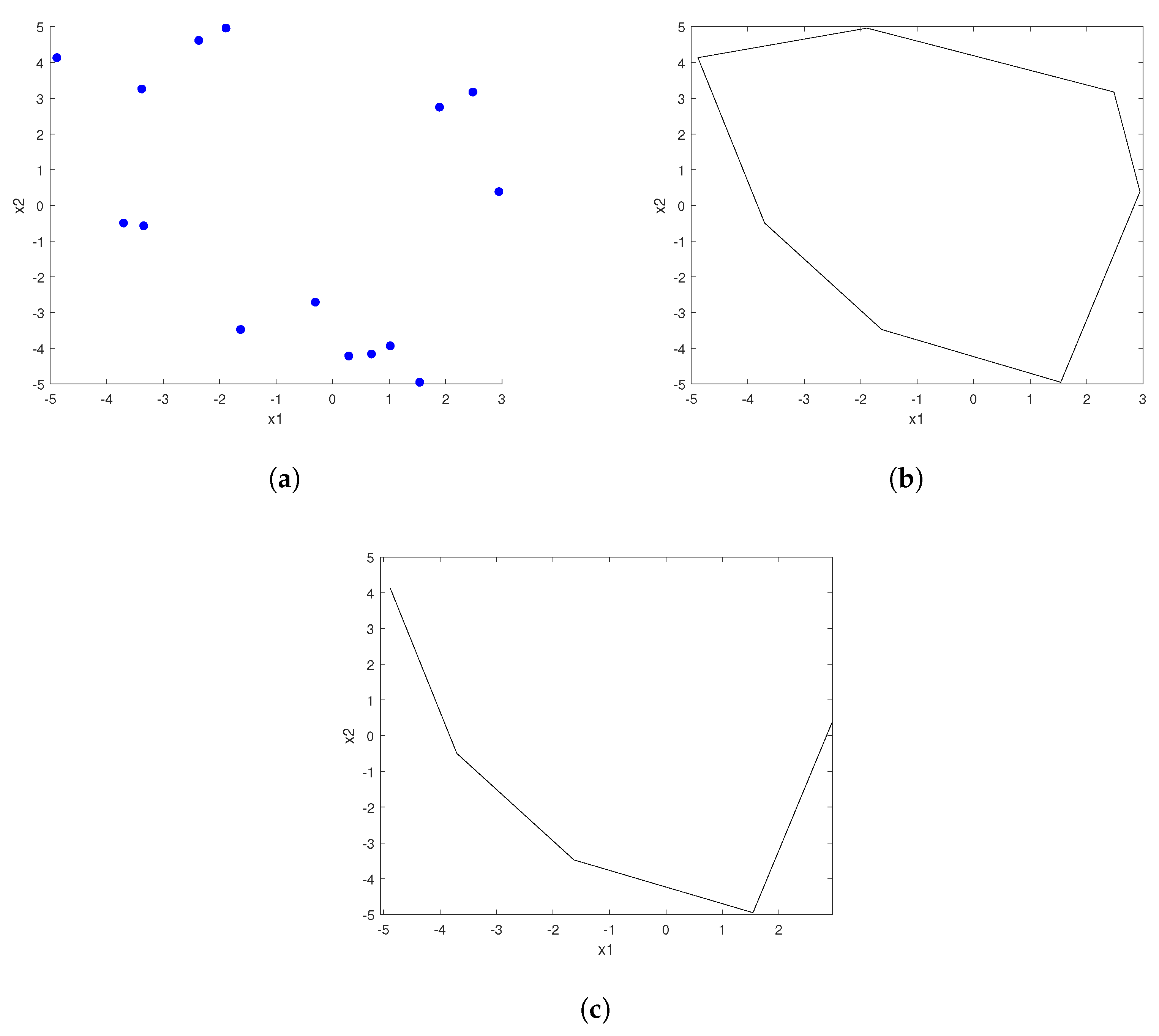
2.1.1. Generate Some Random Points and Use “Quick Hull” Algorithm to Construct a Convex Hull

In the d-dimensional hyperspace ${\mathbb{R}}^d$, a set of N random points $\mathcal{S}=\{{\mathit{x}}_1,...,{\mathit{x}}_N\}$ is generated from the domain ${\mathcal{D}}_d$, where ${\mathcal{D}}_d$ is an arbitrary convex set and ${\mathit{x}}_i\triangleq (x_{i,1},x_{i,2},...,x_{i,d})$. By applying the “quick hull” algorithm [39], a convex hull is constructed and represented by $\mathcal{H}=\{{\mathcal{P}}_1,...,{\mathcal{P}}_m\}$, where ${\mathcal{P}}_j=\{{\mathit{v}}_1^{(j)},...,{\mathit{v}}_d^{(j)}\}$ is a d-dim polygon (or hyper-polyhedron) with d vertices, and each vertex ${\mathit{v}}_k^{(j)}\triangleq (v_{k,1}^{(j)},v_{k,2}^{(j)},\dots ,v_{k,d}^{(j)})\in \mathcal{S}$. Figure 1b shows an example of constructing a 3D convex hull from random points with a setting of $N=15$, and ${\mathcal{D}}_2={[-5,5]}^2$ is a special case of a convex set, which is also consistent with the settings in BBOB.

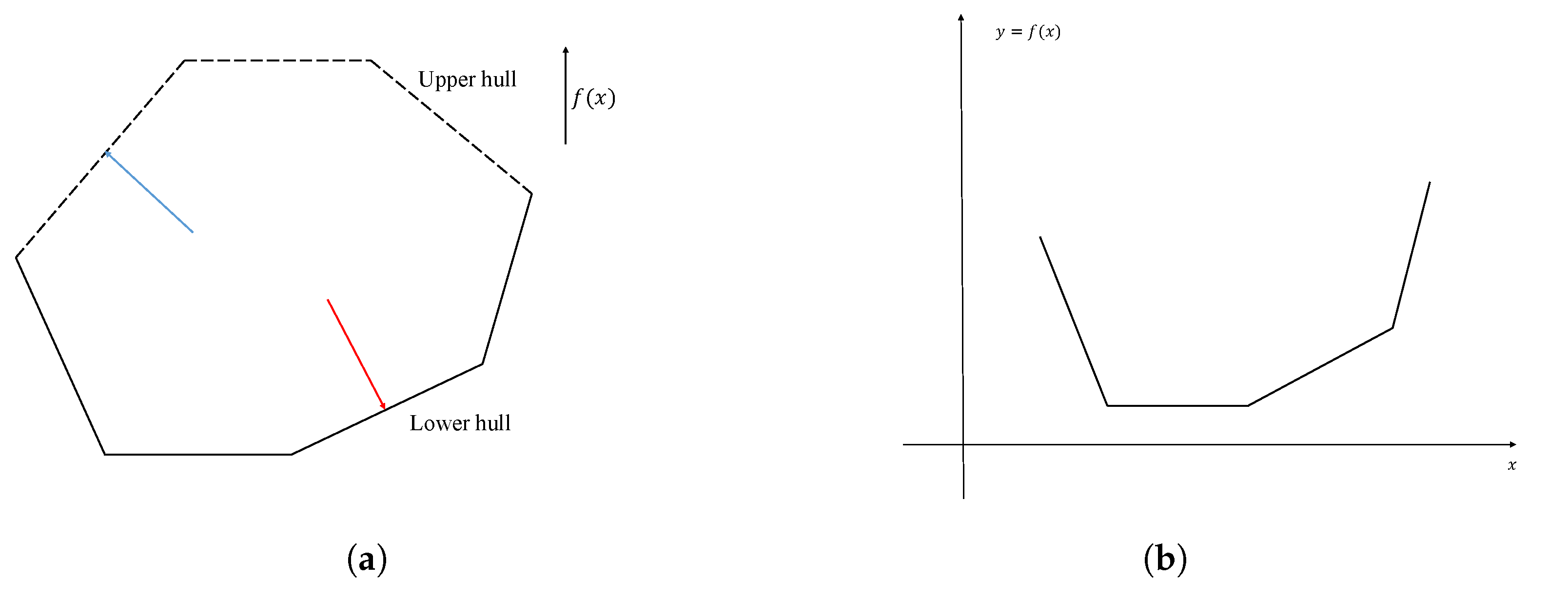
2.1.2. Remove the Upper Hull

For the generated convex hull $\mathcal{H}$, each ${\mathcal{P}}_j$ is identified as belonging to the upper hull or the lower hull. The first step is to find the equation of the hyperplane containing ${\mathcal{P}}_j$ based on the coordinates of the vertices ${\mathit{v}}_k^{(j)}$, for $k=1,2,\dots ,d$.

Let ${\mathcal{A}}_j$ be the hyperplane containing ${\mathcal{P}}_j$. The equation of ${\mathcal{A}}_j$ can be represented as

$$a_{j,1}{x}_1+a_{j,2}{x}_2+\cdots +a_{j,d-1}{x}_{d-1}-x_d+b_j=0.$$

(3)

Note that the coefficient of $x_d$ is set to be $-1$ because later, $x_d$ is set as an explicit function of $x_1,\dots ,x_{d-1}$. Since the d vertices of ${\mathcal{P}}_j$ lie on the hyperplane ${\mathcal{A}}_j$, the other coefficients, $a_{j,1},a_{j,2},\dots ,a_{j,d-1}$ and $b_j$ can be determined by solving a system of d linear equations.

The normal vector ${\mathit{n}}_{\mathit{j}}$ of the hyperplane is ${\mathit{n}}_j=(a_{j,1},a_{j,2},\dots ,a_{j,d-1},-1)$ [43]. To verify whether ${\mathcal{P}}_j$ is an upper or a lower hull, a vector ${\mathit{w}}_{\mathit{j}}$, which starts at a point of the convex hull (but not on ${\mathcal{P}}_j$) and ends at a point in ${\mathcal{A}}_j$, is used to determine the orientation of ${\mathcal{P}}_j$. Pick an arbitrary vertex $\widehat{\mathit{v}}\triangleq ({\widehat{v}}_1,{\widehat{v}}_2,\dots ,{\widehat{v}}_d)\in \mathcal{S}\setminus {\mathcal{P}}_j$ and project it on the hyperplane ${\mathcal{A}}_j$ to obtain the projected point ${\widehat{\mathit{v}}}^{\prime }\triangleq ({\widehat{v}}_1^{\prime },{\widehat{v}}_2^{\prime },\dots ,{\widehat{v}}_d^{\prime })\in {\mathcal{A}}_j$. Thus, ${\mathit{w}}_j$ satisfies two equations:

$$\begin{array}{cc}\hfill {\mathit{w}}_j& ={\widehat{\mathit{v}}}^{\prime }-\widehat{\mathit{v}},\hfill \\ \hfill {\mathit{w}}_j& =\lambda {\mathit{n}}_{\mathit{j}},\hfill \end{array}$$

(4)

where $\lambda$ can be positive or negative. Figure 3 shows the vertex $\widehat{\mathit{v}}$ outside the polygon ${\mathcal{P}}_j$, the projected points ${\widehat{\mathit{v}}}^{\prime }$, and the vector ${\mathit{w}}_j$.

To estimate whether ${\mathcal{P}}_j$ belongs to the upper hull or the lower hull, the key point is to find ${\mathit{w}}_j$. From (4), the projected point ${\widehat{\mathit{v}}}^{\prime }$ can be expressed as

$${\widehat{\mathit{v}}}^{\prime }=\widehat{\mathit{v}}+\lambda {\mathit{n}}_{\mathit{j}}=\left\{\begin{array}{ccc}\hfill {\widehat{v}}_1^{\prime }& =\hfill & \hfill {\widehat{v}}_1+a_{j,1}\lambda ,\\ \hfill {\widehat{v}}_2^{\prime }& =\hfill & \hfill {\widehat{v}}_2+a_{j,2}\lambda ,\\ \hfill ⋮\\ \hfill {\widehat{v}}_d^{\prime }& =\hfill & \hfill {\widehat{v}}_d-\lambda .\end{array}\right.$$

(5)

Since ${\widehat{\mathit{v}}}^{\prime }$ satisfies the equation of ${\mathcal{A}}_j$, $\lambda$ can be solved as

$$\lambda =\frac{{\widehat{v}}_d-b_j-({\widehat{v}}_1{a}_{j,1}+{\widehat{v}}_2{a}_{j,2}+\cdots +{\widehat{v}}_{d-1}{a}_{j,d-1})}{a_{j,1}^2+a_{j,2}^2+\cdots +a_{j,d-1}^2+1}.$$

(6)

Let ${\mathit{u}}_d\triangleq (0,0,\dots ,0,1)$ be the standard unit vector parallel to the $x_d$-axis. Whether ${\mathcal{P}}_j$ belongs to the upper hull or the lower hull can be determined by checking the sign of the inner product ${\mathit{w}}^T{\mathit{u}}_d$. If ${\mathit{w}}^T{\mathit{u}}_d>0$, then the angle between the two vectors is between 0 and $\frac{\pi }{2}$ and ${\mathcal{P}}_j$ is a polygon belonging to the upper hull. Otherwise, it belongs to the lower hull. The convex hull $\mathcal{H}$ is then partitioned into two subsets, the upper hull and the lower hull, denoted by ${\mathcal{H}}_U$ and ${\mathcal{H}}_L$, respectively. The lower hull ${\mathcal{H}}_L$ is an important constituent for constructing the convex function.

The convex landscape ${\mathcal{H}}_L$ is the combination of M hyperplanes ${\mathcal{H}}_L=\{{\mathcal{P}}_1,...,{\mathcal{P}}_M\}$, where M is the total number of polygons. Note that the hyperplanes of the polygons can be extended. Thus, the convex landscape can be constructed.

2.1.3. Computational Complexity

The computational complexity of the offline process is the sum of all the steps. The first step is the constitution of a convex hull via the “quick hull” algorithm. When $d\le 3$, the computational complexity is $O(NlogN)$. When $d>3$, the computational complexity is $O(M)$, where M is the number of polygons of the convex hull [39].

The time complexity from Section 2.1.2 is $O(M{d}^3)$ since all polygons are checked once and their coefficients are determined by solving a system of d linear equations, which has a time complexity of $O(d^3)$, assuming that Gaussian elimination is used [44].

Therefore, the overall time complexity of the offline process is dominated by the process in Section 2.1.2 and is of complexity $O(M{d}^3)$.

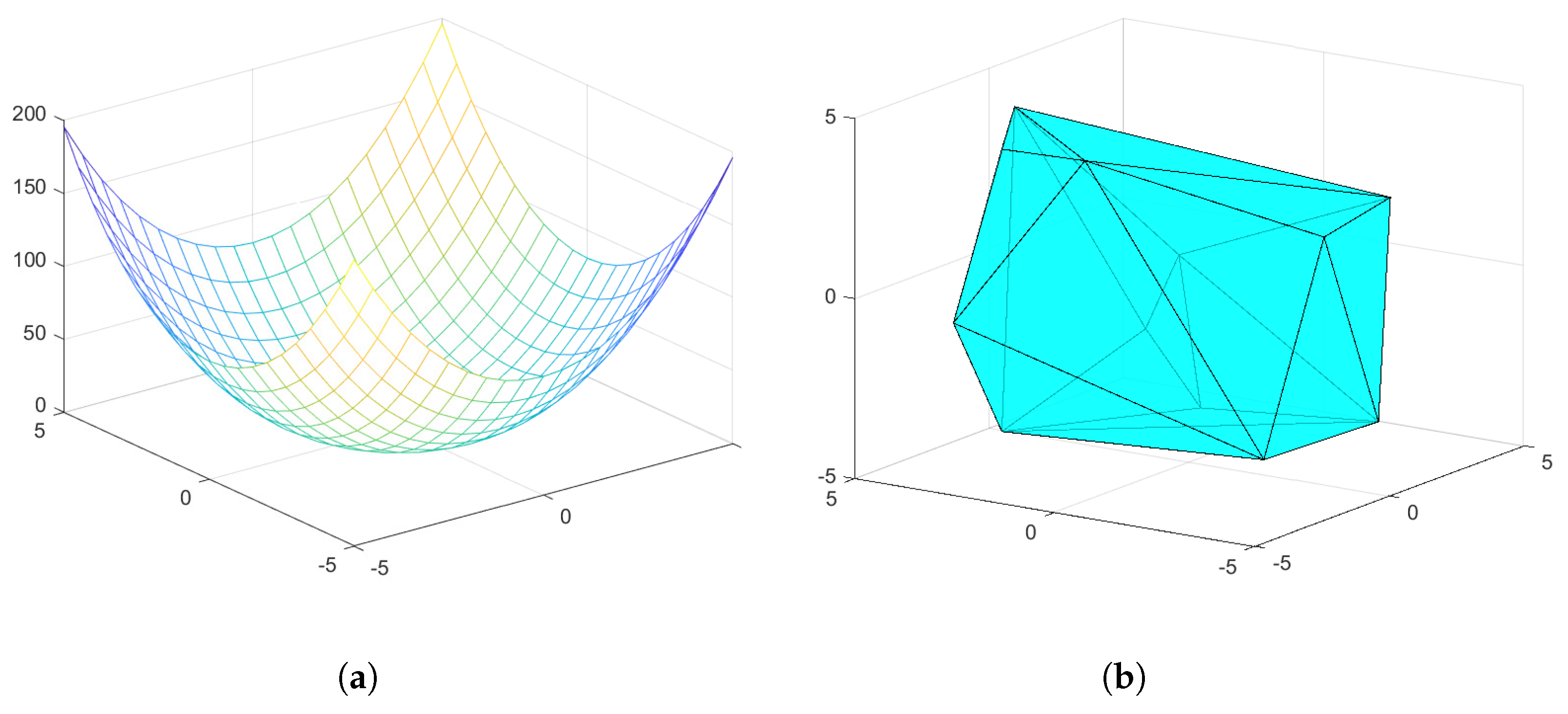
2.1.4. Examples of the Landscape Construction

Two examples show the process of landscape construction for $d\in \{2,3\}$. Figure 4 and Figure 5 illustrate the case of $d=2,N=15$ and the case of $d=3,N=15$, respectively. For each case, sub-figures (a)–(c) show the steps of the landscape construction from a set of random points. When $d>3$, the landscape cannot be visualized anymore. Then, the landscape characteristics are verified in Section 3.2.

2.2. Fitness Evaluation (Online Process)

This section demonstrates the online process, which is the fitness evaluation step for a given input point. In practice, the number of online process executions is determined by the user-defined evaluation budget. Note that this is a query process and given a $(d-1)$-dimensional input $\mathit{x}\in {\mathcal{D}}_{d-1}$, the process returns $f(\mathit{x})$.

The convex landscape is constructed from the perspective of computational geometry starting from arbitrary points. In the process, the fitness of the landscape can be obtained based on the positional relationship between the planes in the space. For any ${\mathcal{A}}_j$ from the lower hull ${\mathcal{H}}_L$, the equation $g_j(\mathit{x})$ to obtain the fitness value of any hyperplane ${\mathcal{A}}_j$ is

$$g_j(\mathit{x})=a_{j,1}{x}_1+a_{j,2}{x}_2+\cdots +a_{j,d-1}{x}_{d-1}+b_j.$$

(7)

Given any input $\mathit{x}$, the fitness value can be evaluated by the following equation:

$$f(\mathit{x})=max\{g_1(\mathit{x}),g_2(\mathit{x}),\dots ,g_M(\mathit{x})\}.$$

(8)

Since $g_j$ is linear, the operation of taking the maximum of (8) ensures the convexity of the landscape since taking the maximum of a set of convex functions preserves the convexity [2].

In the online evaluation process, the computational complexity depends on the structure of the convex hull from the offline process. In the setting in Section 2.1.3, assume that the total number of polygons is M. The relationship between the number of input points, N, and the number of polygons, M, is discussed in the experiment in Section 3.1.

The complexity of (7) is $O(Md)$ since each equation has d terms. The complexity of (8) is $O(M)$. Therefore, the total complexity of the online process is $O(Md)$.

3. Experiments

This section reports three experiments conducted to evaluate the performance of the newly proposed generator. The first experiment investigated the relationship between the number of initial points and the number of polygons. Since $d>3$, the convex function landscape could not be visualized. The second experiment verified the convexity of the multi-dimensional convex landscape. The third experiment used the BFGS algorithm to solve the generated convex function from BBOB and the new generator. All the algorithms and benchmarks in the experiments were coded in Matlab 2021 on a PC with an Intel 3.4 GHz Core I7 processor with 24 GB RAM.

3.1. Relationship between the Number of Vertices N and the Number of Polygons M

The relationship between the number of initial points N and the number of polygons M was investigated. Note that the landscape construction was carried out one time only and was conducted offline. The number of polygons and the time used for the landscape construction were recorded for two different scenarios: (1) $N=d+5$ and (2) $N=2d$. The range of d was set as shown in Figure 6 and Figure 7. One thousand different landscapes were constructed for each scenario and the average numbers were calculated to reflect the trend.

The results shown in Figure 6 and Figure 7 reflect the trend in the number of polygons with the change in the dimensions. When the dimensions increased, the number of polygons increased rapidly. Meanwhile, the number of initial points also affected the number of polygons. With the same dimensions, when the number of initial points was larger, the number of polygons was larger. For example, when $d=10$, Figure 6 shows a setting of $N=15$, whereas Figure 7 shows a setting of $N=20$. In Figure 7, M is much larger than in Figure 6. With more polygons used to construct the landscape, the landscape was more complex. Therefore, the landscape can be tuned by the number of initial points.

3.2. Verifying the Convexity in High Dimensions by the Nonconvexity Measure of the Landscape

The convexity of the generated landscape is straightforward to prove. Since the composed polygons are linear hyperplanes and the composition rule takes the maximum among all the hyperplanes, the generated landscape is convex since taking the maximum of a set of convex functions preserves convexity [2].

In the EC community, convexity is a feature used to evaluate the optimization problem landscape. A practical method, “nonconvex ratio analysis”, was proposed [40] to test the convexity of the landscape. This method randomly samples points and their midpoints from the landscape as a quantitative measure of nonconvexity. The nonconvexity ratio (NCR value) of the landscape is estimated from the sampled points’ fitness values and their midpoint.

In

Table 1. The NCR values of problem instances from BBOB and the proposed generator at different dimensions.

Dimension	Problem of BBOB	NCR Value	N	NCR Value
	f1	0	10	0
d = 2	f7	0.0912	12	0
	f21	0.4804	15	0
	f1	0	10	0
d = 5	f6	0.0448	12	0
	f16	0.4616	15	0
	f1	0	12	0
d = 10	f7	0.0096	14	0
	f15	0.0016	15	0

, the NCR value of the instances from BBOB and those from the generator are illustrated. The instances of the BBOB problem were randomly selected. Note that the selection of the instances was not important. The instances were rotation and translation applied to the basic functions, showing illustrative examples to analyze the convexity of the landscape. To test the new proposed generator, the experiment was conducted with multiple dimensions and various settings of the initial points. Note that when applying nonconvexity measures to analyze the landscape, the landscape was considered a black-box function. The result of instances from the new generator was zero, showing that the generated landscape was always convex. In contrast, the NCR values of BBOB problems were not always zero, depending on which function in the BBOB was selected. The only exception was f1, which was the sphere function. It had an NCR value of zero.

3.3. Using the BFGS Algorithm to Solve the Convex Function

The experiment utilized the BFGS optimization algorithm to solve the generated landscape. The experiments solved the convex function with different dimensions. To implement the BFGS algorithm, the built-in Matlab function “fmincon” was applied.

Figure 8 shows an illustrative example in which the BFGS algorithm solved the generated convex landscape iteratively when $d=3$. The fitness curve shows the progress of the BFGS algorithm in finding the global minimum point in the landscape.

Two examples of the progress of the BFGS algorithm in solving convex problems in high dimensions are illustrated in Figure 9a (for $d=6$) and Figure 9b (for $d=11$).

The BFGS algorithm was also applied to solve the sphere function of BBOB [3]. From Figure 10, it can be seen that the BFGS algorithm took a smaller number of iterations to converge to the optimum of the sphere function class with dimensions of $d=6$ and $d=11$. For example, when $d=6$, the BFGS algorithm solved the problem from the new proposed generator in 113 iterations as shown in Figure 9a, whereas it took 13 iterations to solve the randomly selected f1 instance, as shown in Figure 10a. From the perspective of consuming iterations/time, the landscape from the new proposed generator required a higher evaluation budget for the BFGS algorithm to solve, which intuitively indicates that the problems offered by the new generator are more complex.

4. Conclusions

This paper proposes a novel convex landscape generator that can generate arbitrary d-dimensional convex landscape from an initial set of d-dimensional random points. It works by constructing the convex hull and then extracting the lower boundary of the hull. This lower boundary forms a convex function. It is a “non-parametric” convex function generator as it generates an arbitrary convex landscape from a set of initial random points and does not have any parameters.

It is not based on defining an initial set of convex basis functions and a set of composition rules. Thus, it has no bias toward a particular set of convex basis functions or a particular mathematical form of convex functions.

The construction of the convex function is of the complexity $O(M{d}^3)$, where M is the number of polygons generated. This is an offline process and is executed once only. For a benchmark function query, which is an online process, the complexity is $O(Md)$. It was found that M increases nonlinearly with d as well as N. The process may be time-consuming when both d and N are high.

This convex function landscape generator gives a new class of convex benchmarks for testing the performance of evolutionary algorithms, which is much more general than the rudimentary sphere function benchmark in BBOB and CEC, which allows only simple transformations such as translation and rotation.

The nonconvexity ratio test verifies that the proposed generator indeed generates convex landscapes. Testing using the BFGS, a gradient descent-type algorithm, verifies that the generator generates more challenging convex landscapes than the BBOB sphere function with its limited set of transformations.

Apart from evolutionary computation, the proposed convex landscape generator can be a useful tool for general mathematics and engineering research.

References

1. Taylan, P.; Weber, G.W.; Beck, A. New approaches to regression by generalized additive models and continuous optimization for modern applications in finance, science and technology. Optimization 2007, 56, 675–698. [Google Scholar] [CrossRef]
2. Boyd, S.; Boyd, S.P.; Vandenberghe, L. Convex Optimization; Cambridge University Press: Cambridge, UK, 2004. [Google Scholar]
3. Hansen, N.; Auger, A.; Ros, R.; Mersmann, O.; Tušar, T.; Brockhoff, D. COCO: A platform for comparing continuous optimizers in a black-box setting. Optim. Methods Softw. 2021, 36, 114–144. [Google Scholar] [CrossRef]
4. Liang, J.; Qu, B.; Suganthan, P.; Hernández-Díaz, A.G. Problem Definitions and Evaluation Criteria for the CEC 2013 Special Session on Real-Parameter Optimization; Technical Report; Computational Intelligence Laboratory, Zhengzhou University, China and Nanyang Technological University: Singapore, 2013. [Google Scholar]
5. Suganthan, P.; Hansen, N.; Liang, J.; Deb, K.; Chen, Y.P.; Auger, A.; Tiwari, S. Problem Definitions and Evaluation Criteria for the CEC 2005 Special Session on Real-Parameter Optimization; Technical Report; Nanyang Technological University: Singapore, 2005. [Google Scholar]
6. Gallagher, M.; Yuan, B. A general-purpose tunable landscape generator. IEEE Trans. Evol. Comput. 2006, 10, 590–603. [Google Scholar] [CrossRef] [Green Version]
7. Rönkkönen, J.; Li, X.; Kyrki, V.; Lampinen, J. A framework for generating tunable test functions for multimodal optimization. Soft Comput. 2011, 15, 1689–1706. [Google Scholar] [CrossRef]
8. Das, S.; Suganthan, P. Problem Definitions and Evaluation Criteria for CEC 2011 Competition on Testing Evolutionary Algorithms on Real World Optimization Problems; Technical Report; Jadavpur University: Kolkata, India, 2011. [Google Scholar]
9. Karaboga, D.; Akay, B. A comparative study of artificial bee colony algorithm. Appl. Math. Comput. 2009, 214, 108–132. [Google Scholar] [CrossRef]
10. Kennedy, J.; Eberhart, R. Particle swarm optimization. In Proceedings of the ICNN’95—International Conference on Neural Networks, Perth, WA, Australia, 27 November–1 December 1995; Volume 4, pp. 1942–1948. [Google Scholar]
11. Das, S.; Suganthan, P.N. Differential evolution: A survey of the state-of-the-art. IEEE Trans. Evol. Comput. 2010, 15, 4–31. [Google Scholar] [CrossRef]
12. Salawudeen, A.T.; Mu’azu, M.B.; Yusuf, A.; Adedokun, A.E. A Novel Smell Agent Optimization (SAO): An extensive CEC study and engineering application. Knowl.-Based Syst. 2021, 232, 107486. [Google Scholar] [CrossRef]
13. Panwar, D.; Saini, G.; Agarwal, P. Human Eye Vision Algorithm (HEVA): A Novel Approach for the Optimization of Combinatorial Problems. In Artificial Intelligence in Healthcare; Springer: Berlin/Heidelberg, Germany, 2022; pp. 61–71. [Google Scholar]
14. Hansen, N. The CMA evolution strategy: A comparing review. In Towards a New Evolutionary Computation; Springer: Berlin/Heidelberg, Germany, 2006; pp. 75–102. [Google Scholar]
15. Fletcher, R. Practical Methods of Optimization; John Wiley & Sons: Hoboken, NJ, USA, 2013. [Google Scholar]
16. Finck, S.; Hansen, N.; Ros, R.; Auger, A. Real-Parameter Black-Box Optimization Benchmarking 2009: Presentation of the Noiseless Functions; Technical Report; Citeseer: Princeton, NJ, USA, 2010. [Google Scholar]
17. Kerschke, P.; Trautmann, H. Automated algorithm selection on continuous black-box problems by combining exploratory landscape analysis and machine learning. Evol. Comput. 2019, 27, 99–127. [Google Scholar] [CrossRef] [Green Version]
18. Mersmann, O.; Bischl, B.; Trautmann, H.; Preuss, M.; Weihs, C.; Rudolph, G. Exploratory landscape analysis. In Proceedings of the 13th Annual Conference on GENETIC and Evolutionary Computation, Dublin, Ireland, 12–16 July 2011; pp. 829–836. [Google Scholar]
19. Malan, K.M.; Engelbrecht, A.P. A survey of techniques for characterising fitness landscapes and some possible ways forward. Inf. Sci. 2013, 241, 148–163. [Google Scholar] [CrossRef] [Green Version]
20. Malan, K.M.; Engelbrecht, A.P. Fitness landscape analysis for metaheuristic performance prediction. In Recent Advances in the Theory and Application of Fitness Landscapes; Springer: Berlin/Heidelberg, Germany, 2014; pp. 103–132. [Google Scholar]
21. Muñoz, M.A.; Smith-Miles, K.A. Performance analysis of continuous black-box optimization algorithms via footprints in instance space. Evol. Comput. 2017, 25, 529–554. [Google Scholar] [CrossRef]
22. Muñoz, M.A.; Smith-Miles, K. Generating new space-filling test instances for continuous black-box optimization. Evol. Comput. 2020, 28, 379–404. [Google Scholar] [CrossRef] [PubMed]
23. Lou, Y.; Yuen, S.Y. On constructing alternative benchmark suite for evolutionary algorithms. Swarm Evol. Comput. 2019, 44, 287–292. [Google Scholar] [CrossRef]
24. Biswas, S.; Das, S.; Suganthan, P.N.; Coello, C.A.C. Evolutionary multiobjective optimization in dynamic environments: A set of novel benchmark functions. In Proceedings of the 2014 IEEE Congress on Evolutionary Computation (CEC), Beijing, China, 6–11 July 2014; pp. 3192–3199. [Google Scholar]
25. Gee, S.B.; Tan, K.C.; Abbass, H.A. A benchmark test suite for dynamic evolutionary multiobjective optimization. IEEE Trans. Cybern. 2016, 47, 461–472. [Google Scholar] [CrossRef] [PubMed]
26. Jiang, S.; Kaiser, M.; Yang, S.; Kollias, S.; Krasnogor, N. A scalable test suite for continuous dynamic multiobjective optimization. IEEE Trans. Cybern. 2019, 50, 2814–2826. [Google Scholar] [CrossRef] [PubMed]
27. Li, C.; Nguyen, T.T.; Zeng, S.; Yang, M.; Wu, M. An open framework for constructing continuous optimization problems. IEEE Trans. Cybern. 2018, 49, 2316–2330. [Google Scholar] [CrossRef] [PubMed]
28. Kudela, J.; Matousek, R. New Benchmark Functions for Single-Objective Optimization Based on a Zigzag Pattern. IEEE Access 2022, 10, 8262–8278. [Google Scholar] [CrossRef]
29. Yazdani, D.; Omidvar, M.N.; Cheng, R.; Branke, J.; Nguyen, T.T.; Yao, X. Benchmarking continuous dynamic optimization: Survey and generalized test suite. IEEE Trans. Cybern. 2020, 52, 3380–3393. [Google Scholar] [CrossRef]
30. Yazdani, D.; Cheng, R.; Yazdani, D.; Branke, J.; Jin, Y.; Yao, X. A survey of evolutionary continuous dynamic optimization over two decades—Part B. IEEE Trans. Evol. Comput. 2021, 25, 630–650. [Google Scholar] [CrossRef]
31. Dullerud, G.E.; Paganini, F. A Course in Robust Control Theory: A Convex Approach; Springer Science & Business Media: Berlin/Heidelberg, Germany, 2013; Volume 36. [Google Scholar]
32. Hardy, G.H.; Littlewood, J.E.; Pólya, G. Inequalities; Cambridge University Press: Cambridge, UK, 1952. [Google Scholar]
33. Kim, C.E.; Rosenfeld, A. Digital straight lines and convexity of digital regions. IEEE Trans. Pattern Anal. Mach. Intell. 1982, 149–153. [Google Scholar] [CrossRef]
34. Kim, C.E.; Rosenfeld, A. Convex digital solids. IEEE Trans. Pattern Anal. Mach. Intell. 1982, PAMI-4, 612–618. [Google Scholar] [CrossRef]
35. Chassery, J.M.; Garbay, C. An iterative segmentation method based on a contextual color and shape criterion. IEEE Trans. Pattern Anal. Mach. Intell. 1984, PAMI-6, 794–800. [Google Scholar] [CrossRef] [PubMed]
36. Lin, M.C.; Manocha, D.; Cohen, J.; Gottschalk, S. Collision Detection: Algorithms and applications. In Algorithms for robotic Motion and Manipulation; Citeseer: Princeton, NJ, USA, 1997; pp. 129–142. [Google Scholar]
37. O’Rourke, J. Computational Geometry in C; Cambridge University Press: Cambridge, UK, 1998. [Google Scholar]
38. Jarvis, R.A. On the identification of the convex hull of a finite set of points in the plane. Inf. Process. Lett. 1973, 2, 18–21. [Google Scholar] [CrossRef]
39. Barber, C.B.; Dobkin, D.P.; Huhdanpaa, H. The quickhull algorithm for convex hulls. ACM Trans. Math. Softw. (TOMS) 1996, 22, 469–483. [Google Scholar] [CrossRef] [Green Version]
40. Tamura, K.; Gallagher, M. Quantitative measure of nonconvexity for black-box continuous functions. Inf. Sci. 2019, 476, 64–82. [Google Scholar] [CrossRef]
41. Gray, A.; Abbena, E.; Salamon, S. Modern Differential Geometry of Curves and Surfaces with Mathematica®; Chapman and Hall/CRC: Boca Raton, FL, USA, 2017. [Google Scholar]
42. Mark, d.B.; Otfried, C.; Marc, v.K.; Mark, O. Computational Geometry Algorithms and Applications; Spinger: Berlin/Heidelberg, Germany, 2008. [Google Scholar]
43. Gellert, W.; Hellwich, M.; Kästner, H.; Küstner, H. The VNR Concise Encyclopedia of Mathematics; Springer Science & Business Media: Berlin/Heidelberg, Germany, 2012. [Google Scholar]
44. Lay, D.C. Linear Algebra and Its Applications; Pearson Education India: Delhi, India, 2003. [Google Scholar]
Figure 1. Two examples of a convex function landscape and convex hull. (a) This is an example of a composed convex function f ( x 1 , x 2 ) = ( ( x 1 ) 2 + ( x 2 ) 2 + 0.1 ) log ( ( x 1 ) 2 + ( x 2 ) 2 + 0.1 ) (b) This is an example of a convex hull when d = 3 .
Mathematics 10 03974 g001
Figure 2. Constructing a convex function from the convex hull when d = 3 . (a) Upper hull and lower hull of a convex hull (b) The convex function is formed by extracting the lower hull.
Mathematics 10 03974 g002
Figure 3. An example of vertex v ^ outside the polygon P j , the projected points v ^ , and the vector w j . In addition, n j is the normal vector of P j and u d is the standard unit vector parallel to the x d -axis.
Mathematics 10 03974 g003
Figure 4. Constructing the convex function landscape when d = 2 , N = 15 . (a) Randomly generated points. (b) Constructed convex hull. (c) The curve after removing the upper hull.
Mathematics 10 03974 g004
Figure 5. Constructing the convex function landscape when d = 3 , N = 15 . (a) Randomly generated points in 3D space. (b) Constructed convex hull. (c) The remaining lower hull H L after removing the upper hull.
Mathematics 10 03974 g005
Figure 6. Relationship between the number of initial points N and the number of polygons M when the initial number of polygons is N = d + 5 .
Mathematics 10 03974 g006
Figure 7. Relationship between the number of initial points N and the number of polygons M when the initial number of polygons is N = 2 d .
Mathematics 10 03974 g007
Figure 8. Applying BFGS algorithm to solve the generated convex function landscape when d = 3 . (a) The figure is a randomly generated convex function landscape. (b) Searching curve shows the progress of solving the optimization problem.
Mathematics 10 03974 g008
Figure 9. (a) The fitness curve for the BFGS algorithm when searching for the optimum of the generated problem when d = 6 , N = 15 . (b) The fitness curve for the BFGS algorithm when searching for the optimum of the generated problem when d = 11 , N = 15 .
Mathematics 10 03974 g009
Figure 10. (a) The fitness curve for the BFGS algorithm when d = 6 for a BBOB problem instance randomly selected from the f1 class. (b) The fitness curve for the BFGS algorithm when d = 11 for a BBOB problem instance randomly selected from the f1 class.
Mathematics 10 03974 g010