Abstract
This paper aims to test the structure of interest rates during the period from 1 September 1981 to 28 December 2020 by using Lie algebras and groups. The selected period experienced substantial events impacting interest rates, such as the economic crisis, the military intervention of the USA in Iraq, and the COVID-19 pandemic, in which economies were in lockdown. These conditions caused the interest rate to have a nonlinear structure, chaotic behavior, and outliers. Under these conditions, an alternative method is proposed to test the random and nonlinear structure of interest rates to be evolved by a stochastic differential equation captured on a curved state space based on Lie algebras and group. Then, parameter estimates of this equation were obtained by OLS, NLS, and GMM estimators (hereafter, LieNLS, LieOLS, and LieGMM, respectively). Therefore, the interest rates that possess nonlinear structures and/or chaotic behaviors or outliers were tested with LieNLS, LieOLS, and LieGMM. We compared our LieNLS, LieOLS, and LieGMM results with the traditional OLS, NLS, and GMM methods, and the results favor the improvement achieved by the proposed LieNLS, LieOLS, and LieGMM in terms of the RMSE and MAE in the out-of-sample forecasts. Lastly, the Lie algebras with NLS estimators exhibited the lowest RMSE and MAE followed by the Lie algebras with GMM, and the Lie algebras with OLS, respectively.
Keywords:
interest rate; Lie groups; Lie algebras; stochastic differential equation; OLS; NLS; GMM; LieNLS; LieOLS; LieGMM MSC:
22E60; 22E70; 17B45
1. Introduction
Although the interest rate term structure has been discussed by many articles in the literature, there are only a few articles analyzing this structure by the Lie method which provide the connection among the symmetry groups and the integrability properties of differential equations (DEs) [1]. In the recent literature, the Lie methods (Lie algebras and groups) have had a deep influence on mathematics, mechanics, and robotics science branches. Modeling the interest rates with differentiable manifold bases was studied by a few papers in pursuit of [2,3,4,5,6], which provide examples of a short rate model on the circle S1. Ref. [7] explored the random and nonlinear structure of interest rates on S1 and S2 manifolds using matrix representations.
Hughston [8] is an important paper that develops a model for arbitrage-free pricing on general Riemann manifolds. Kusuoka [9] developed high-order discretization schemes of SDEs by using free Lie algebra. Other studies using the Lie method, including [10], were aimed at utilizing the partial differential equations (PDEs), and [11] used PDEs in the multidimensional screening problem, and [12] used PDEs for financial models with non-linear state spaces. In the context of the financial diffusion models, Morimoto and Sasada [13] suggested the Lie method on vector fields. Bildirici et al. [14] and Muniz et al. [15] aimed to solve financial mathematics problems by applying the Lie method. Ref. [15] suggested time-dependent correlation matrices for solving SDE that evolves in the special orthogonal group.
In this paper, we aim to analyze the short-term interest rate models on the S2 manifold during the period of 1 September 1981 to 28 December 2020 via matrix representations of Lie algebras for the US. The analyzed period is important because it encompasses some significant economic factors, such as economic crises, and non-economic factors, such as COVID-19, the USA intervention in Iraq, etc. The unexpected movements of oil prices and locked-down markets throughout the World have driven governments to increase their aid to stop the downfall of markets. These factors led the interest rates to exhibit a different structure than the usual, which was the effect of the pandemic and the large-scale fiscal expansion that occurred in response to it. During the period of COVID-19, the premium term for US government bonds changed. The difference in yield between US government bonds with a maturity of 2 to 10 years is the definition of “premium”. Since 1 April, treasury bonds have been in a downward trend, trading below 0.15% with 1-year maturity. The interest rate structure and behavior were affected in this process. It exhibited nonlinear and/or chaotic behavior.
Under this condition, the Ordinary Stochastic Differential Equation for interest rates was expressed by matrix representations of Lie groups and Lie algebras. Then, parameter estimation of this equation was obtained by OLS, NLS, and GMM methods. Therefore, the nonlinear models were defined by the Stochastic Differential Equation via the Lie method. We also obtained the parameter estimates for this equation using OLS, NLS, and GMM (hereafter, LieOLS, LieNLS, and LieGMM) methods. Then, we obtained parameter estimates for the ordinary Stochastic Differential Equation without Lie representations by using OLS, NLS, and GMM methods (hereafter, the traditional OLS, NLS, and GMM). Additionally, the forecast results of two methods were compared with each other. Afterwards, the forecast results of LieOLS, LieNLS, and LieGMM methods are compared with the results derived with the traditional OLS, NLS, and GMM models.
The contribution of the paper is in two ways. In the context of applied mathematics, the paper contributes by the simultaneous utilization of the LieOLS, LieNLS, and LieGMM models to obtain parameter estimations. In the context of financial mathematics, Park et al. [7], Goard [16], Bildirici et al. [14], and Ucan and Bildirici [17] used only the OLS estimation method. This paper used three different methods: OLS, NLS, and GMM. Therefore, a second contribution of the paper is to improvement the efficiency of government policies with the policy recommendations derived following the proposed methods.
2. Methodology: Lie Groups and Algebras
Lie groups, their algebras, and the relation of stochastic dynamics between these groups are presented [7,12,16]. Let G and g be a matrix Lie group with dimensional and its algebra [18]. The orthogonal matrix is denoted by , and is defined as:
Hence, the orthogonal matrix groups are denoted by , and defined as follows:
For these special orthogonal matrix groups, in the case of , the typical element of the group SO(2) is a rotation matrix. The manifold of this group is identified with the unit circle, , with parametrization, .
In the case of , , the typical element of the group (3) is a rotation matrix. The manifold of this group is identified with the unit sphere, , with parametrization, , ,.
Similarly, the manifold of the Lie group is given as .
The Lie algebras of these groups are denoted by . It is provided as for . The relation between the group and this algebra is given by:
2.1. Proposition
If the state equation and the quadratic function are defined, respectively, as follows: , where is a constant, and is the diffusion process,
is a symmetric matrix, then the dynamics for are given in Equation (4):
where , , and is the correlation coefficient between and , where (that is, are components of the diffusion process).
2.2. Short Rate on the Lie Group
The Lie group is a differentiable manifold, and can be identified with the unit sphere, . In this manifold, the short rate and state equation are given as follows:
where .
where are positive symmetric matrices. In the case, the dynamics for function are given with Equation (5):
where:
, , and we can use one of the following forms for the matrix element of :
Since the dynamics on are , their stochastic equations are derived from Equation (5). Then, the equation for each dynamic is solved. Therefore, the short rate, , is obtained as follows:
where:
and
where .
3. Data and Results
The data are historical daily US Treasury interest rates covering the 1 November 1981–28 December 2020 period with various maturities: 3 and 6 months; and, 1, 5, 10, 20, and 30 years. Data were taken from FRED (https://fred.stlouisfed.org (5 May 2021)). The interest rate variables with the above-mentioned maturities are shown in Figure 1. As the figure shows, the movement of variables follows a similar path.
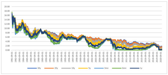
Figure 1.
Interest rates for the various maturities. Source: FRED.
As mentioned in Section 2, the state equation is given as:
where the Wiener process is , .
For the three-factor short rate model on , the following equation is used:
where both are symmetric positive–definite, thereby ensuring that s always remains positive. The stochastic differential equation for s can be derived from Equation (7).
The model parameters are in the underlying state equations; the symmetric positive definite matrices, , are used to define the short rate; and the 3 × 3 covariance matrix, W, is associated with the Wiener process. The published interest rates, , are the spot rates. The spot rates can be obtained via the expectation as follows:
. It is interest rate at time, t, for the length of maturity, .
The Monte Carlo simulation was employed to directly evaluate the above expectation. The ordinary least-squares (OLS), nonlinear least-squares (NLS), and generalized method of moments (GMM) estimation procedures were used for parameter estimation in a three-factor short rate model on . Choose an initial set of parameters, ). The covariance matrix for the Wiener process is assumed to be W. Generate a sufficient number of sample paths for the short rate, and determine the time series for all the spot rates; denote the estimated spot rate data by (see [7,14,17] for similar app.). Determine if the choice of model parameters is an optimizer for the objective function:
’s are historical time series data of spot rates for the following maturities: 3 months(M), 6 M, 1 year(Y), 2Y, 3Y, 5Y, 7Y, 10Y, 20Y, and 30Y.
The results will be obtained with the following five steps. (1). Descriptive statistics and unit root tests will be applied. By the unit root test, the stationarity of the variables will be investigated. (2). Lyapunov and Tsay tests are applied to determine the evidence of chaotic and nonlinear behavior of the interest rates. (3). The Lie methods with OLS, NLS, and GMM estimators, namely, LieOLS, LieNLS, and LieGMM, are applied. The results are compared with those obtained from the traditional OLS, NLS, and GMM models. (4). For in-sample, the forecasts results obtained from the Lie method are compared with the forecast results of the traditional models. Further, the out-of-sample forecast results will be obtained for 10, 20, and 30 working days ahead. (5). The Diebold–Mariano test is applied (assuming the forecast error criteria as the RMSE to evaluate the performance of the proposed Lie-based methods.
4. Results
Firstly, the descriptive statistics of the spot rates of all maturities were obtained. Table 1 shows the results of the descriptive statistics. The main problem is not much excess skewness, but excess kurtosis.

Table 1.
Descriptive statistics.
Since the Tsay NL test determined the nonlinearities of the variables, the ADF test and the KSS test, as important tests in the evidence of nonlinear variables, were employed to explore the stationary. ADF and KSS unit root tests determined the stationary at the level for the variables in Table 2.
Table 2.
Unit root tests.
The results of the Tsay and Lyapunov tests in Table 3 are presented. The Tsay nonlinearity test suggests that the linearity is misspecified for the variables.
Table 3.
Lyapunov * and Tsay Tests.
The maximum Lyapunov (λ) results found a chaotic structure with values between 0 < λ < 1, since the positive values of the Lyapunov test showed evidence of chaos [21]. In the state that the variables have a chaotic and nonlinear structure, LieOLS, LieNLS, and LieGMM models allow us to analyze models that are difficult to analyze.
4.1. Lie Method Results
The results of the Lie method are presented in Table 4. We considered a three-factor short rate model on . The short rate, , is always positive and is obtained from Equation (5).
Table 4.
Estimations of Lie parameters with OLS, NLS, and GMM methods *.
To test the goodness-of-fit of the model, we calculated the skewness and kurtosis of the error between the actual and the estimated short rates by employing the 3M maturity spot rate as proxy (the figures are not presented here).
In the whole period, the kurtosis and skewness of the errors for LieOLS were determined as 3.18 and −0.5516, respectively. The kurtosis and skewness of the errors for LieNLS were determined as 3.34 and −0.63, and 3.11 and −0.513 for LieGMM, respectively.
In Table 4, the estimations of Lie parameters with OLS, NLS, and GMM methods are presented.
4.2. Forecast Results
The results of the in-sample and out-of-sample were compared. Since the lowest RMSE and MAE coefficients in the in-sample and out-of-sample results are considered as the best result, the model that gives these results will be accepted as the most successful. The results of the in-sample and out-of-sample forecasts are given in Table 5 and Table 6, respectively.
Table 5.
In-sample forecast results.
Table 6.
Out-of-sample forecast results.
Table 5 shows the results of Lie methods with OLS, NLS, and GMM, and the results of traditional models using OLS, NLS, and GMM methods.
Lie methods with OLS, NLS, and GMM provide better results than traditional methods. RMSE and MAE results determined by Lie methods with OLS, NLS, and GMM are smaller than those determined by traditional methods. RMSE and MAE values determined by traditional NLS and LieNLS are smaller than the others within their own groups.
4.3. The Results of the Out-of-Sample Forecast
In Table 6, the MAE and RMSE results for Lie methods with NLS, OLS, and GMM were obtained to search their forecast accuracy for 10, 20, and 30 workdays ahead (shown as T + 10, T + 20, and T + 30, respectively). According to the results of the out-of-sample, the Lie method with NLS exhibited the lowest RMSE, followed by the Lie method with GMM.
4.4. To Test for Forecast Accuracy
The Diebold–Mariano (DM) test results are shown in Table 7, and the p-values are given. If the p-value is <0.05, the H0 hypothesis was rejected. Three models were compared in the terms of RMSE performance.
Table 7.
Diebold–Mariano results.
Firstly, among the models, when RMSELieOLS is compared with RMSELieNLS, and when RMSELieOLS is compared with RMSELieGMM, we fail to reject the H0 hypothesis of equal forecast accuracy. We also compared the RMSELieNLS model with the RMSELieOLS and RMSELieGMM models. The H0 hypothesis is rejected in favor of the RMSELieNLS model. The results show that the RMSELieNLS model is preferred over the RMSELieOLS and RMSELieGMM models.
5. Conclusions
This paper aimed to analyze the interest rates for the period from 1 September 1981 to 28 December 2020 by using the Lie method with OLS, NLS, and GMM estimators for the US. In the literature, interest rate term structure models generally aimed to determine the nonlinear structure of interest rates. Some of them covered nonlinear stochastic state dynamics evolving on a vector space. Refs. [2,7,21] tested the interest rate models in the context of the Lie method. As a differentiation from these papers, in this paper, we suggested LieOLS, LieGMM, and LieNLS models in the context of the drift and noise volatility terms of stochastic state equations. Firstly, we explored chaotic and nonlinear structures. Secondly, the evidence of nonlinear and chaotic structures of the variables, and the suggested Lie methods with OLS, NLS, and GMM estimators determined the parameter estimates. Thirdly, the results of LieOLS, LieGMM, and LieNLS models were compared with those of traditional OLS, NLS, and GMM methods. Then, the forecast results of in-sample and out-of-sample were obtained. The forecasting results of in-sample were compared with results of traditional estimators. According to the results of the Lie method, traditional estimators exhibited low forecasting performance. Lastly, we applied Diebold–Mariano tests in terms of RMSE performance. The results determined that the RMSELieNLS model has better performance over the RMSELieOLS and RMSELieGMM models. According to our results, employing the Lie methods caused a rising forecasting performance in the existence of the nonlinear structure. The lie method is a good estimator. For this reason, the use of the Lie method in the solution of the stochastic problem, which is difficult to solve, can provide significant improvements. This is very important in the context of policy recommendations. The results of the Lie method, in comparison with the traditional methods, can allow us to make the best decision in the context of policy recommendations.
As a suggestion for future papers, the usage of this method to solve open problems in applied mathematics, economics, and financial mathematics will provide important contributions. On the other hand, because the use of supersymmetries in engineering and physics is common and very important, using the fractional super group, SU(2), which is one of the real forms of the fractional super group, SL(2,C), obtained in Ucan and Kosker [22], to solve this model is suggested in future papers.
Author Contributions
Conceptualization, M.B.; methodology, Y.U.; software, M.B., Y.U. and S.L.; validation, M.B. and Y.U.; formal analysis, Y.U.; investigation, Y.U.; resources, M.B. and Y.U.; data curation, M.B., Y.U. and S.L.; writing—original draft preparation, M.B. and Y.U.; writing—review and editing, M.B. and Y.U.; visualization, M.B., Y.U. and S.L.; supervision, M.B. and Y.U.; project administration, M.B., Y.U. and S.L.; funding acquisition, S.L. All authors have read and agreed to the published version of the manuscript.
Funding
This research received no external funding.
Data Availability Statement
Data are freely available from FRED.
Conflicts of Interest
The authors declare no conflict of interest.
References
- Lie, S. Über die integration durch bestimmte integrate von einer klasse linearer partieller differentialgleichungen. Arch. Math. Nat. 1881, 6, 328–368. [Google Scholar]
- Nunes, J.; Webber, N.J. Low Dimensional Dynamics and the Stability of HJM Term Structure Models; Working Paper; University of Warwick: Coventry, UK, 1997. [Google Scholar]
- Gazizov, R.K.; Ibragimov, N.H. Lie symmetry analysis of differential equations in finance. Nonlinear Dyn. 1998, 17, 387–407. [Google Scholar] [CrossRef]
- Ibragimov, N.H.; Wafo Soh, C. Solution of the Cauchy problem for the Black-Scholes equation using its symmetries, Modern Group Analysis. In Modern Group Analysis, International Conference at the Sophus Lie Conference Center; Ibragimov, N.H., Naqvi, K.R., Straume, E., Eds.; MARS Publishers: Nordfjordeid, Norway, 1997. [Google Scholar]
- Lo, C.F.; Hui, C.H. Valuation of financial derivatives with time-dependent parameters: Lie-algebraic approach. Quant. Financ. 2001, 1, 73–78. [Google Scholar] [CrossRef]
- Carr, P.; Lipton, A.; Madan, D. The Reduction Method for Valuing Derivative Securities; Working Paper; New York University: New York, NY, USA, 2002. [Google Scholar]
- Park, F.C.; Chun, C.M.; Han, C.W.; Webber, N. Interest rate models on Lie groups. Quant. Financ. 2011, 11, 559–572. [Google Scholar] [CrossRef]
- Hughston, L. Stochastic Differential Geometry, Financial Modelling, and Arbitrage-Free Pricing; Working Paper; Merrill Lynch: New York, NY, USA, 1994. [Google Scholar]
- Kusuoka, S. Approximation of expectation of diffusion process based on Lie algebra and Malliavin calculus. Adv. Math. Econ. 2004, 6, 69–83. [Google Scholar]
- Polidoro, S. A nonlinear PDE in mathematical finance. In Numerical Mathematics and Advanced Application; Brezzi, F., Buffa, A., Corsaro, S., Murli, A., Eds.; Springer: Milano, Italy, 2003; pp. 429–433. [Google Scholar]
- Basov, S. Lie groups of partial differential equations and their application to the multidimensional screening problems. Univ. Melb. Econ. Work. Pap. 2004. [Google Scholar] [CrossRef]
- Webber, N. Valuation of financial models with non-linear state spaces. AIP Conf. Proc. 2001, 553, 315–320. [Google Scholar]
- Morimoto, Y.; Sasada, M. Algebraic Structure of Vector Fields in Financial Diffusion Models and its Applications. Quant. Financ. 2017, 17, 1105–1117. [Google Scholar] [CrossRef][Green Version]
- Bildirici, M.; Bayazit, N.G.; Ucan, Y. Modelling Oil Price with Lie Algebras and Long Short-Term Memory Networks. Mathematics 2021, 9, 1708. [Google Scholar] [CrossRef]
- Muniz, M.; Ehrhardt, M.; Günther, M. Approximating Correlation Matrices Using Stochastic Lie Group Methods. Mathematics 2021, 9, 94. [Google Scholar] [CrossRef]
- Goard, J. New solutions to the bond-pricing equation via Lie’s classical method. Math. Comput. Model. 2000, 32, 299–313. [Google Scholar] [CrossRef]
- Ucan, Y.; Bildirici, M. Air Temperature Measurement Based on Lie Group SO(3). Therm. Sci. 2022, 26, 3089–3095. [Google Scholar] [CrossRef]
- Vilenkin, N.J.; Klimyk, A.U. Representations of Lie Groups and Special Functions: Recent Advances; Kluwer Academic Publishers: Dordrecht, The Netherlands, 1991; Volume 1. [Google Scholar]
- Sivakumar, B. Is a chaotic multi-fractal approach for rainfall possible? Hydrol. Process. 2001, 15, 943–955. [Google Scholar] [CrossRef]
- Bildirici, M. Chaotic Dynamics on Air Quality and Human Health: Evidence from China, India, and Turkey. Nonlinear Dyn. Psychol. Life Sci. 2021, 52, 207–237. [Google Scholar]
- Bildirici, M. Chaos Structure and Contagion Behavior between COVID-19, and the Returns of Prices of Precious Metals and Oil: MS-GARCH-MLP Copula. Nonlinear Dyn. Psychol. Life Sci. 2022, 26, 209–219. [Google Scholar]
- Ucan, Y.; Kosker, R. The Real Forms of The Fractional Supergroup SL (2,C). Mathematics 2021, 9, 933. [Google Scholar] [CrossRef]

Publisher’s Note: MDPI stays neutral with regard to jurisdictional claims in published maps and institutional affiliations. |
© 2022 by the authors. Licensee MDPI, Basel, Switzerland. This article is an open access article distributed under the terms and conditions of the Creative Commons Attribution (CC BY) license (https://creativecommons.org/licenses/by/4.0/).