An SDP Dual Relaxation for the Robust Shortest-Path Problem with Ellipsoidal Uncertainty: Pierra’s Decomposition Method and a New Primal Frank–Wolfe-Type Heuristics for Duality Gap Evaluation

Abstract

This work addresses the robust counterpart of the shortest path problem (RSPP) with a correlated uncertainty set. Because this problem is difficult, a heuristic approach, based on Frank–Wolfe’s algorithm named discrete Frank–Wolfe (DFW), has recently been proposed. The aim of this paper is to propose a semi-definite programming relaxation for the RSPP that provides a lower bound to validate approaches such as the DFW algorithm. The relaxed problem is a semi-definite programming (SDP) problem that results from a bidualization that is done through a reformulation of the RSPP into a quadratic problem. Then, the relaxed problem is solved by using a sparse version of Pierra’s decomposition in a product space method. This validation method is suitable for large-size problems. The numerical experiments show that the gap between the solutions obtained with the relaxed and the heuristic approaches is relatively small.

1. Introduction

Robust combinatorial optimization consists of taking uncertainty into account in combinatorial optimization problems. For instance, the robust shortest path problem is the problem of finding the shortest route from one place to another, whereas the distance (either in terms of time or space) of the different parts of the road are uncertain. Many definitions of robustness have been proposed in the literature in the context of optimization. The three most common definitions in the context of combinatorial optimization have been formalized in [1]. These are the absolute robust solution, the robust deviation and the relative robust solution. In all these cases, worst-case behavior is considered. For these three definitions, an uncertainty set has to be defined. Many uncertainty sets exist, such as interval uncertainty, discrete uncertainty, and ellipsoidal uncertainty [2]. Another family of definitions is scenario-dependent. In these methods, a decision is taken conditionally on the current scenario and the overall optimization problem boils down to a robust two-stage problem [3]. This family splits into the notions of K-adaptability [4], adjustable robustness, bulk robustness, and recoverable robustness. In the case in which the data can be considered as governed by a certain probability distribution with unknown parameters, distributionally robust optimization [5] is also an interesting approach. It consists of choosing the distribution that is most suitable given a robustness criterion. Yet another approach is the notion of the almost robust solution [6], which is feasible under most of the realizations and that can use full, partial, or no probabilistic information about the uncertain data. Let us also mention that other alternative generic approaches have also been proposed in the literature. In [7], a near-optimum solution for several scenarios is proposed. Another way to tackle uncertainty that is different from robust optimization is online optimization [8], whereby decisions are made iteratively, and at each iteration, the problem inputs are unknown, but the decision maker learns from the previous configuration before making his decision. After a decision is made, it is then assessed against the optimal one. Finally, let us add that uncertainty theory was used in another line of work, as in [9] for instance. This theory has also been implemented in [10] in order to give what they call an uncertainty distribution in the case of the shortest-path problem.

This work considers the absolute robust decision with the uncertainty in the cost function modeled by an ellipsoidal uncertainty set. The choice of the ellipsoidal uncertainty set is motivated as follows. Unlike the interval uncertainty set, it takes the correlation of the uncertain variables into account, reduces the combinatorial aspect of the discrete set, and allows the user to control the level of risk that he is ready to take in order to have the right cost. Finally, it leads to a smooth form for the min-max formulation, as shown in Section 2.1. This smooth form is well-known in portfolio optimization, and is called mean-risk optimization [11]. In [1], it is demonstrated that the robust counterparts of easy problems are usually hard to solve, especially if the uncertainty set is not an interval, but is described by an ellipsoidal confidence region. In this case, the robust counterparts of even linear problems become non-linear. To solve these NP-hard problems, methods exist for the case of non-correlated variables, i.e., for axis-parallel ellipsoids [12,13,14,15]. In the case of correlated variables, branch-and-bound methods exist, as well as improvements by better node relaxations [16]. A heuristic approach called discrete Frank–Wolfe (DFW) for robust optimization under correlated ellipsoidal uncertainty based on Frank–Wolfe’s algorithm has been proposed in [17]. To the best of our knowledge, it is the first algorithm for robust optimization in the ellipsoidal uncertainty adapted for large-size problems.

In order to validate heuristic approaches, one can compare other exact or heuristic methods, give sub-optimality proofs, or compute lower/upper bounds depending on whether it is a minimization or a maximization problem. For minimization problems, lower bounds can be obtained by using relaxation schemes such as the ones obtained by using Lagrangian dualizations [18] which often result in solving semi-definite programming (SDP) problems.

SDP is a particular class of convex optimization problems which appears in various engineering-motivated problems, including the most efficient relaxations of some NP-hard problems such as those often encountered in combinatorial optimization or mixed-integer programming [19]. SDP can be written as minimization over symmetric (resp. Hermitian) positive semi-definite matrix variables, with linear cost function and affine constraints, i.e., problems of the form

$$\begin{array}{c}\hfill \underset{Z⪰0}{min}\left(A•Z:B_j•Z=b_j\mathrm{for}j=1,\dots ,m\right),\end{array}$$

(1)

where $A,B_1,\dots ,B_m$ are given matrices, $Z⪰0$ stands for a symmetric matrix Z being positive semi-definite, and • is the inner product defined by

$$A•B=tr(A^{T}B)$$

(2)

for square matrices A and B. Compact SDPs can be solved in polynomial time. SDP was extensively studied over the last three decades since its early use, which can be traced back to [20,21]. In particular, linear matrix inequalities (LMI) and their numerous applications in control theory, system identification, and signal processing have been a central drive for the use of SDP in the 1990’s as reflected in the book [22]. One of the most influential papers of that era, is [23], in which SDP was shown to provide a 0.87 approximation to the max-cut problem, a famous clustering problem on graphs. Other SDP schemes for approximating hard combinatorial problems have subsequently been devised for the graph coloring problem [24] and for the satisfiability problem [23,25]. These results were later surveyed in [26,27,28]. Numerical methods for solving SDPs are manifold, and various schemes have been devised for specific structures of the constraints. One of these families of methods is the class of interior point methods [29]. Such methods are known to be accurate, but suffer from a lack of scalability in practice. Another family of methods is based on the alternating direction method of multipliers (ADMM) technique [30]. ADMM approaches are usually faster as they can be implemented in a distributed architecture. As such, they often appear to be faster and more scalable than interior point methods at the price of worse accuracy. Other methods can also be put to work as the method of Pierra [31] upon which the present work further elaborates.

In this work, the quality of the solution of the DFW heuristic approach is evaluated by computing a lower bound for a given problem instance. This lower bound is obtained by a bidualization of the robust problem, which is an SDP relaxation. In order to solve the corresponding SDP problem, the applied method is the decomposition through formalization into a product space proposed in [31], with a sparse computation to reduce the memory storage necessity. It is shown that this algorithm is a validation method that is also applicable to large-size problems.

The paper is organized as follows. Section 2 presents the robust shortest-path problem, and recalls two approaches to solve the problem; in particular we oppose the exact solving branch-and-bound method of CPLEX to an efficient heuristic algorithm, the so-called DFW algorithm, proposed in a previous paper [17] that is scalable and performs well on simulations. Because the exact approach is costly, the main contribution of this paper is to propose a validation method for DFW by an efficient relaxation method that provides a lower bound for the cost function. This is described in Section 3. Finally, Section 4 numerically validates this approach by showing that the corresponding gap between the solutions obtained with the relaxed and the proposed heuristic approaches is small.

Notation. Throughout the paper, the following matrix notations have been used. Unless stated otherwise, all vectors belonging to ${\mathbb{R}}^l$ for some $l\in {\mathbb{N}}^{*}$ are column vectors. Furthermore, for some matrix M, $M[a:b,c:d]$ denotes, for all integers $a\le b$ and $c\le d$, the sub-block containing the entries in the rows a to b and columns c to d. $M[a,c:d]$ (resp. $M[a:b,c]$) is short for $M[a:a,c:d]$ (resp. $M[a:b,c:c]$). $M^T$ is the transpose of M. $S^d$ denotes the set of symmetric matrices of size $d\times d$. Finally, $0_{(l,l)}$ is the block of dimension $l\times l$ with zeros everywhere and $I_l$ is the identity block of dimension $l\times l$.

2. The Robust Shortest-Path Problem

In this section, the robust shortest-path problem with the ellipsoidal uncertainty set is stated. The problem form to solve is then given in order to propose a robust solution. Both an exact and a heuristic method for solving this problem are presented.

2.1. Problem Statement

Consider the linear programming form of the shortest-path problem [32], which can be written as

$$\begin{array}{c}\hfill \underset{x\in X}{min}{c}^{T}x,\end{array}$$

(3)

with $c\in {\mathbb{R}}^m$ being the cost vector and $X=\{x\in {\{0,1\}}^m;Ax=b\}$, where $A\in {\mathbb{R}}^{n\times m}$ is the so-called incidence matrix corresponding to the underlying graph, and $b\in {\mathbb{R}}^n$ is the vector with n entries that defines the source node and the destination node (see Section IV.A in [17] for more details).

This paper considers the particular situation where the cost vector $c\in {\mathbb{R}}^m$ is uncertain, i.e., lies in an uncertainty set $U\subseteq {\mathbb{R}}^m$. Then, the robust counterpart of Problem (3) is the following:

$$\begin{array}{c}\hfill \underset{x\in X}{min}\underset{c\in U}{max}{c}^{T}x.\end{array}$$

(4)

In the particular case in which the cost vector c is a random vector following a multinormal distribution with expectation $\mu \in {\mathbb{R}}^m$ and covariance matrix $\sum \in {\mathbb{R}}^{m\times m}$, then c belongs to the confidence set E with probability $(1-\alpha )\in [0,1]$, where E is the following ellipsoid:

$$\begin{array}{c}\hfill E=\{c\in {\mathbb{R}}^m;{(c-\mu )}^T{\sum }^{-1}(c-\mu )\le {\mathsf{\Omega }}^2\},\end{array}$$

(5)

with $\mathsf{\Omega }={\mathsf{\Omega }}_{\alpha }\ge 0$ being a function of $\alpha$ that represents the level of confidence. More precisely, ${\mathsf{\Omega }}_{\alpha }={\chi }_m^2(1-\alpha )$ and ${\chi }_m^2(1-\alpha )$ refers to the quantile function for probability $1-\alpha$ of the chi-squared distribution with m degrees of freedom (see Section 3.1 in [33]).

One interesting fact about the ellipsoidal uncertainty set is that the min-max problem (4) can be reduced to a non-linear programming problem (for more details see Section 2.2.1.1 of [34]):

$$\begin{array}{c}\hfill \underset{x\in X}{min}\underset{c\in E}{max}{c}^{T}x=\underset{x\in X}{min}{\mu }^{T}x+\mathsf{\Omega }\sqrt{x^T\sum x}.\end{array}$$

(6)

Without loss of generality, it is assumed throughout this paper that $\mathsf{\Omega }=1$, so that Problem (6) reads

$$\begin{array}{c}\hfill \underset{x\in X}{min}{\mu }^{T}x+\sqrt{x^T\sum x}=\underset{x\in X}{min}g(x),\end{array}$$

(7)

where $g(x)={\mu }^{T}x+\sqrt{x^T\sum x}$. It is easy to transform a general problem in the form (6) to the case $\mathsf{\Omega }=1$ by a change of variable ${\sum }^{{}^{\prime }}={\mathsf{\Omega }}^2\sum$, so we have the equivalence

$$\underset{x\in X}{min}{\mu }^{T}x+\mathsf{\Omega }\sqrt{x^T\sum x}=\underset{x\in X}{min}{\mu }^{T}x+\sqrt{x^T{\sum }^{{}^{\prime }}x}.$$

The remaining part of this section addresses the robust shortest-path problem by solving Problem (7). This problem is a non-linear non-convex problem, so it is challenging to find an appropriate method by which to solve it.

2.2. Exact Method for Solving the Robust Problem

In order to solve the robust shortest-path problem, solving Problem (7) is needed. One possible way is to solve this problem in two steps. First, rewrite it as a binary second order cone programming problem (BSOCP) (see Problem (8)). The solution is obtained by solving Problem (8) in the second step. Problem (8) is stated as follows:

$$\begin{array}{cc}\hfill min& {\mu }^{T}x+z\hfill \\ \hfill \mathrm{s}.\mathrm{t}.& {(y,z)}^T\in K_{m+1}\hfill \\ \hfill & y={({\sum }^{\frac{1}{2}})}^{T}x\hfill \\ \hfill & x\in X,y\in {\mathbb{R}}^m,z\in {\mathbb{R}}_{+},\hfill \end{array}$$

(8)

with the second order cone $K_{m+1}$ defined as

$$K_{m+1}:=\{x\in {\mathbb{R}}^{m+1};\parallel {(x_1,\dots ,x_m)}^T{\parallel }_2\le x_{m+1}\}.$$

(9)

The calculations are detailed in Section 4 in [17].

Problem (8) can be solved by branch-and-bound methods, and existing BSOCP solvers such as CPLEX [35] are able to solve this problem. However, for large size problems, it is no longer possible to use branch-and-bound methods, because their time complexity is exponential, and in their worst case, they may need to explore all the possible permutations of the combinatorial problem at hand. Thus, a heuristic algorithm named the DFW algorithm has been proposed in [17] and is presented in the following section.

2.3. A Heuristic Approach Based on Frank–Wolfe

As proven in the previous section, solving the robust shortest-path problem with a scalable heuristic approach seems mandatory for large-size problems. The heuristic algorithm proposed in [17] to solve Problem (7) is based on the Frank–Wolfe algorithm [36]. The proposed heuristic approach is only valid because the shortest-path problem has the following particular property: using the simplex algorithm, it is possible to find a binary solution that solves the linear problem over the convex hull. This is the case because the incidence matrix A is totally unimodular [37]. The steps of the DFW algorithm are the following. On one side, the classical Frank–Wolfe (FW) algorithm is a convex optimization algorithm that proceeds by moving toward a minimizer of the linear approximation of the function to minimize. The heuristic DFW algorithm in turn uses the classical Frank–Wolfe algorithm to minimize $g(x)={\mu }^{T}x+\sqrt{x^T\sum x}$ over the convex hull of X, and due to the integrality of the relaxation with the simplex algorithm, the intermediate gradient steps are feasible solutions for the discrete problem. These gradient steps are good feasible solutions. The DFW algorithm returns the best of these intermediate steps as an approximate solution: more concretely, it is the one that minimizes the objective function g among the discovered feasible solutions. The stopping criteria has been chosen as the convergence of the relaxed problem. No proof about the convergence of the heuristics DFW can be given; it is indeed only a heuristics. The DFW algorithm is detailed in Algorithm 1.

Algorithm 1 DFW: a Frank–Wolfe based algorithm to solve (7)

1: $x^{(0)}$ a random feasible solution, $\epsilon >0$ close to zero, K the maximum number of iterations. 2: $k\leftarrow 1$ 3: stop ← false 4: while $k\le K$ and ¬stop do 5:    if $g(x^{(k-1)})-g(x^{(k)})<\epsilon$ then 6:      stop ← true 7:    else 8:        Choose ${\displaystyle s^{(k)}\in \underset{y\in \mathrm{Conv}(X)}{argmin}\nabla g{(x^{(k)})}^{T}y,\mathrm{with}{s}^{(k)}\in X}$ 9:        ${\displaystyle {\gamma }^{(k)}\leftarrow \underset{\alpha \in [0,1]}{argmin}g(x^{(k)}+\alpha (s^{(k)}-x^{(k)}))}$ 10:        $x^{(k+1)}\leftarrow x^{(k)}+{\gamma }^{(k)}(s^{(k)}-x^{(k)})$ 11:    end if 12:    $k++$ 13: end while 14: return${\displaystyle \underset{s\in \{s^{(1)},\dots ,s^{(k-1)}\}}{argmin}g(s)}$

Note $x^{*}$ the optimal solution of Problem (7), and $\widehat{x}$ the approximate solution given by the DFW algorithm. The aim of the next section is to evaluate the quality of the solution $\widehat{x}$.

3. A Lower Bound by SDP Relaxation

The first way to evaluate the quality of an actual result of the DFW algorithm, or any other approach that solves Problem (7), is to compare it with the solution given by the optimal solution, up to numerical precision, of the BSOCP by using an exact solver like CPLEX (see the previous section). Because this approach is no longer usable when considering the large sized problem, an other option to evaluate the quality of the solution has to be proposed. To do so, a lower bound by bidualization, with a memory efficient algorithm to solve the corresponding problem, is presented in this section.

3.1. Bidualization of a Quadratic Problem

Before giving a lower bound for Problem (7), a lower bound by bidualization for any quadratic problem is stated. Then, Problem (7) is written as a quadratic problem following the general form.

A lower bound for quadratic programming problems in general form is proposed in [26]. This lower bound is the solution of a bidual problem that is written in the form of an SDP problem. It turns out that this bidualization procedure is nothing but the very known SDP relaxation. In the following, we give a review of the relevant parts of Section 4 of [26] that has all the ingredients of bidualization of a quadratic problem, and to ease the understanding for the reader, we give the references of every equation and proposition taken from [26].

Consider the quadratic problem (Problem (21) in [26]) with N constraints:

$$\begin{array}{c}\hfill inf{q}_0(x),x\in {\mathbb{R}}^d\\ \hfill q_j(x)=0,j=1,\dots ,N,\end{array}$$

(10)

where

$$q_j(x)=x^T{Q}_{j}x+b_j^{T}x+c_j,j=0,\dots N$$

are $N+1$ quadratic functions defined on ${\mathbb{R}}^d$, $d\in {\mathbb{N}}^{*}$ being the dimension of the problem, with the matrices $Q_j$ lying in the set $S^d$ of symmetric matrices of size $d\times d$, the values $b_j$ in ${\mathbb{R}}^d$, and the values $c_j$ in $\mathbb{R}$$\forall j\in \{1,2,\dots ,N\}$; it is assumed that $c_0=0$.

Applying Lagrangian duality on Problem (10), and applying duality again reproduces the bidual problem of (10) (Problem (SDP) in Theorem 4.4 of [26]), which is given by

$$\begin{array}{c}\hfill inf{Q}_0•X+b_0^{T}x,X\in S^d,x\in {\mathbb{R}}^d,\\ \hfill Q_j•X+b_j^{T}x+c_j=0,j=1,\dots ,N,\\ \hfill \left[\begin{array}{cc}1& x^T\\ x& X\end{array}\right]⪰0,\end{array}$$

(11)

where we recall that the inner product between the matrices A and B of size $d\times d$ is defined by (2), and the notation $M⪰0$ means that M is positive semi-definite, for any symmetric matrix M.

This bidualization has another interpretation: it is also a direct convexification of Problem (10). Indeed, noticing that (10) can also be written as

$$\begin{array}{c}\hfill inf{Q}_0•X+b_0^{T}x,X\in S^d,x\in {\mathbb{R}}^d,\\ \hfill Q_j•X+b_j^{T}x+c_j=0,j=1,\dots ,N,\\ \hfill X=x{x}^T\end{array}$$

(12)

by setting $X=x{x}^T$, and writing a quadratic form $x^{T}Qx$ as $Q•x{x}^T$, and then relaxing the nonconvex constraint $X=x{x}^T$ to $X⪰x{x}^T$, that is convex with respect to $(x,X)$. Then, the previous bidualization can be seen as a convexification in ([26], Section 4.4).

Thus, if $p^{*}$ is the optimal solution of (10), and $d^{**}$ is the optimal solution of (11), then the following inequality holds (see Proposition 4.5 in [26]):

$$d^{**}\le p^{*}.$$

(13)

Hence, solving the SDP problem (11) enables us to obtain a lower bound for $p^{*}$. In general, this technique is used for the validation of a heuristic method without comparison with the optimal solution. In this case, Problem (11) is easier, because it is a convex problem. Solving (11) gives the lower bound $d^{**}$. The distance between the lower bound and the heuristic solution can bound however far this heuristic solution is from the optimal solution. In other research directions, the lower bound can be coupled with a branch-and-bound algorithm for computing an optimal solution. However, the focus in the present paper is on proposing a much cheaper heuristics than the branch-and-bound approach, namely the DFW method. In order to validate this heuristics, the quality of the obtained primal solution using a lower bound obtained by solving a polynomial time SDP problem has been evaluated.

3.2. Applying This Bidualization to Compute a Lower Bound for the Robust Shortest-Path Problem

This section aims to show how to use the bidualization, explained in Section 3.1, to compute a lower bound for Problem (7).

3.2.1. Bidualization of the Addressed Problem

Recall that Problem (7) has another formulation, which is a BSOCP (Problem (8)). By using the definition (9) for $K_{m+1}$, we may rewrite (8) explicitly as follows:

$$\begin{array}{cc}\hfill min& {\mu }^{T}x+z\hfill \\ \hfill \mathrm{s}.\mathrm{t}.& \sqrt{y^{T}y}\le z\hfill \\ \hfill & y={({\sum }^{\frac{1}{2}})}^{T}x\hfill \\ \hfill & x\in X,y\in {\mathbb{R}}^m,z\in {\mathbb{R}}_{+}.\hfill \end{array}$$

(14)

First, the BSOCP formulation (14) of (7) can be written as a binary quadratic problem (BQP) because the variables y and z in (14) are such that $\sqrt{y^{T}y}\ge 0$ and $z\ge 0$ for any $y\in {\mathbb{R}}^m$ and $z\in {\mathbb{R}}_{+}$. Thus, Problem (14) is equivalent to

$$\begin{array}{cc}\hfill min& {\mu }^{T}x+z\hfill \\ \hfill \mathrm{s}.\mathrm{t}.& y^{T}y\le z^2\hfill \\ \hfill & y={({\sum }^{\frac{1}{2}})}^{T}x\hfill \\ \hfill & x\in X,y\in {\mathbb{R}}^m,z\in {\mathbb{R}}_{+}.\hfill \end{array}$$

(15)

In order to formulate (15) as a problem in the form (10), all the constraints must be written in the form of equalities. First, the following equivalence holds:

$$x\in X\iff Ax=b\mathrm{and}x\in {\{0,1\}}^m\iff Ax=b\mathrm{and}{x}_i(x_i-1)=0i=1,\dots ,m.$$

Secondly, the inequality $y^{T}y\le z$ can be transformed into an equality by considering additional variables $c_1$ and $c_2$ as follows:

$$y^{T}y\le z^2\iff \exists c_1\in \mathbb{R}\mathrm{s}.\mathrm{t}.y^{T}y-z^2=-c_1^2\iff \exists c_1\in \mathbb{R}\mathrm{s}.\mathrm{t}.y^{T}y-z^2+c_1^2=0$$

$$z\ge 0\iff \exists c_2\in \mathbb{R}\mathrm{s}.\mathrm{t}.z=c_2^2\iff \exists c_2\in \mathbb{R}\mathrm{s}.\mathrm{t}.z-c_2^2=0.$$

The problem (15) is then equivalent to the following problem:

$$\begin{array}{cc}\hfill min& {\mu }^{T}x+z\hfill \\ \hfill \mathrm{s}.\mathrm{t}.& y^{T}y-z^2+c_1^2=0\hfill \\ \hfill & y={({\sum }^{\frac{1}{2}})}^{T}x\hfill \\ \hfill & Ax=b\hfill \\ \hfill & x_i(x_i-1)=0i=1,\dots ,m\hfill \\ \hfill & z-c_2^2=0\hfill \\ \hfill & x\in {\mathbb{R}}^m,y\in {\mathbb{R}}^m,z\in \mathbb{R},c_1\in \mathbb{R},c_2\in \mathbb{R}.\hfill \end{array}$$

(16)

Now, Problem (16) is written in a more compact way, i.e., in function of one vector variable $u=[x,y,z,c_1,c_2]\in {\mathbb{R}}^{2m+3}$, and write each constraint individually. This makes Problem (16) equivalent to

$$\begin{array}{cc}\hfill min& {(\tilde{\mu }+{\delta }_{2m+1})}^{T}u\hfill \\ \hfill \mathrm{s}.\mathrm{t}.& u^T({𝟙}_y^T{𝟙}_y-{\delta }_{2m+12m+1}+{\delta }_{2m+22m+2})u=0\hfill \\ \hfill & {({𝟙}_y-({\sum }^{\widetilde{\frac{1}{2}}T}))}_i^{T}u=0i=1,\dots ,m\hfill \\ \hfill & {\tilde{A}}_j^{T}u=b_{j}j=1,\dots ,n\hfill \\ \hfill & u^T{\delta }_{ii}u-{\delta }_i^{T}u=0i=1,\dots ,m\hfill \\ \hfill & -u^T{\delta }_{2m+32m+3}u+{\delta }_{2m+1}^{T}u=0\hfill \\ \hfill & u\in {\mathbb{R}}^{2m+3},\hfill \end{array}$$

(17)

where the vectors and matrices that appear in Problem (17) are defined as follows

• the vector $\tilde{\mu }$ of size $2m+3$ is defined block-wise as $\tilde{\mu }={[\mu ,0,\dots ,0]}^T$, so that ${\tilde{\mu }}^{T}u={\mu }^{T}x$ if $u=[x,y,z,c_1,c_2]$,
• for any $k=1,\dots ,2m+3$, ${\delta }_k\in {\mathbb{R}}^{2m+3}$ is such that ${\delta }_k(l)=1$ if $k=l$, and 0 if else, so that ${\delta }_{2m+1}^{T}u=u_{2m+1}=z$, and ${\delta }_i^{T}u=x_i$ for $i=1,\dots m$,
• ${𝟙}_y$ is an $m\times (2m+3)$ matrix such that ${𝟙}_y[m+1:2m;m+1:2m]=I_m$ and 0 elsewhere, so that ${𝟙}_{y}u=y$ and $u^T{𝟙}_y^T{𝟙}_{y}u=y^{T}y$,
• for any $i,j=1,\dots ,2m+3$, ${\delta }_{i,j}$ is a $(2m+3)\times (2m+3)$ matrix, such that ${\delta }_{i,j}(k,l)=1$ if $i=k$ and $j=l$, and 0 if else. So that $u^T{\delta }_{2m+1,2m+1}u=z^2$, $u^T{\delta }_{2m+2,2m+2}u=c_1^2$, $u^T{\delta }_{2m+3,2m+3}u=c_2^2$ and $u^T{\delta }_{ii}u=u_i^2$ for $i=1,\dots ,m$,
• ${\sum }^{\widetilde{\frac{1}{2}}T}$ is an $m\times (2m+3)$ matrix such that ${\sum }^{\widetilde{\frac{1}{2}}T}[1:m;1:m]={\sum }^{\frac{1}{2}T}$ and the other entries are zeros, so that ${\sum }^{\widetilde{\frac{1}{2}}T}u={\sum }^{\frac{1}{2}T}x$,
• $\tilde{A}$ is an $n\times (2m+3)$ matrix such that $\tilde{A}[1:n;1:m]=A$ and the other entries are zeros, so that $\tilde{A}u=Ax$.

Thus, we have rewritten the problem in form of (10), and the bidual problem of (17) is the following:

$$\begin{array}{cc}\hfill min& {(\tilde{\mu }+{\delta }_{2m+1})}^{T}u\hfill \\ \hfill \mathrm{s}.\mathrm{t}.& ({𝟙}_y^T{𝟙}_y-{\delta }_{2m+12m+1}+{\delta }_{2m+22m+2})•U=0\hfill \\ \hfill & {({𝟙}_y-({\sum }^{\widetilde{\frac{1}{2}}T}))}_i^{T}u=0i=1,\dots ,m\hfill \\ \hfill & {\tilde{A}}_j^{T}u=b_{j}j=1,\dots ,n\hfill \\ \hfill & {\delta }_{ii}•U-{\delta }_i^{T}u=0i=1,\dots ,m\hfill \\ \hfill & -{\delta }_{2m+32m+3}•U+{\delta }_{2m+1}^{T}u=0\hfill \\ \hfill & \left[\begin{array}{cc}1& u^T\\ u& U\end{array}\right]⪰0,U\in S^{2m+3},u\in {\mathbb{R}}^{2m+3}.\hfill \end{array}$$

(18)

The last step consists in writing (18) in a compact way with the following change of variable

$$\begin{array}{c}\hfill Z=\left[\begin{array}{cc}1& u^T\\ u& U\end{array}\right]\in S^{2m+4}.\end{array}$$

This can be done by using the following changes:

(1)

For any $v\in {\mathbb{R}}^{2m+3}$, write $v^{T}u=V•U$, where $V\in S^{2m+4}$ is defined by

$$\begin{array}{c}\hfill V=\frac{1}{2}\left[\begin{array}{ccc}0& |& v^T\\ v& |& 0\end{array}\right]\in S^{2m+4}.\end{array}$$

(2)

For any $W\in S^{2m+3}$, write $W•U=\mathbf{W}•Z$, where $\mathbf{W}\in S^{2m+4}$ is defined by

$$\begin{array}{c}\hfill \mathbf{W}=\left[\begin{array}{ccc}0& |& \dots 0\\ 0& |& W\end{array}\right].\end{array}$$

As a result of this change of variable, the bidual problem of (15) can be written in the form of an SDP problem as in (11) in the more compact way:

$$\begin{array}{cc}\hfill min& M•Z\hfill \\ \hfill \mathrm{s}.\mathrm{t}.& Z\in S^{2m+4}\hfill \\ \hfill & O_j•Z=b_j,j=1,\dots ,n,\hfill \\ \hfill & C_i•Z=0,i=1,\dots ,m,\hfill \\ \hfill & Q•Z=0,\hfill \\ \hfill & D_i•Z=0,i=2,\dots ,m+1\hfill \\ \hfill & L•Z=0,\hfill \\ \hfill & Z⪰0,\hfill \end{array}$$

(19)

where $M\in S^{2m+4}$ is defined as follows:

$$\begin{array}{c}\hfill M=\frac{1}{2}\left[\begin{array}{cc}0& {\mu }^{T}0\dots 0100\\ \mu & \\ 0& \\ ⋮\\ 0& 0\\ 1& \\ 0& \\ 0\end{array}\right],\end{array}$$

that is $M[1,2:m+1]=\frac{1}{2}{\mu }^T$, $M[1,2m+2]=\frac{1}{2}$, $M[2:m+1,1]=\frac{1}{2}\mu$, $M[2m+2,1]=\frac{1}{2}$, and zero elsewhere. Note that in term of sparsity, the number of non-zero entries for M is an $O(m)$. The matrix $O_j\in S^{2m+4}$ is defined for all $j=1,\dots ,n$ by

$$\begin{array}{c}\hfill O_j=\frac{1}{2}\left[\begin{array}{cc}0& A_j^{T}0\dots 0000\\ A_j& \\ 0& \\ ⋮\\ 0& 0\\ 0& \\ 0& \\ 0\end{array}\right],\end{array}$$

that is $O_j[1,2:m+1]=\frac{1}{2}{A}_j^T$, $O_j[2:m+1,1]=\frac{1}{2}{A}_j$, and zero elsewhere. Here, the number of non zero entries for each $O_j$ is an $O(m)$. The matrix $C_i\in S^{2m+4}$ is defined for all $i=1,\dots ,m$ by

$$\begin{array}{c}\hfill C_i=\frac{1}{2}\left[\begin{array}{cc}0& -{({\sum }^{\frac{1}{2}T})}_i^{T}0\dots 010\dots 0\\ -{({\sum }^{\frac{1}{2}T})}_i& \\ 0& \\ ⋮\\ 0& \\ 1& 0\\ 0& \\ ⋮& \\ 0\end{array}\right],\end{array}$$

that is $C_i[1,2:m+1]=-\frac{1}{2}{({\sum }^{\frac{1}{2}T})}_i^T$, $C_i[1,m+1+i]=\frac{1}{2}$, $C_i[2:m+1,1]=-\frac{1}{2}{({\sum }^{\frac{1}{2}T})}_i$, $C_i[m+1+i,1]=\frac{1}{2}$, and zero elsewhere. The matrices $C_i$ have $O(m^2)$ non zero entries. We next define the matrix Q by

$$\begin{array}{c}\hfill Q=\left[\begin{array}{cccccc}0& 0\dots 0& 0\dots 0& 0& 0& 0\\ & 0_{(m,m)}& & & & \\ & & I_m& & & \\ ⋮& & & -1& & \\ & & & & 1& \\ 0& & & & & 0\end{array}\right],\end{array}$$

that is $Q[m+2:2m+1,m+2:2m+1]$ is the identity matrix of dimension m, $Q[2m+2,2m+2]=-1$, $Q[2m+3,2m+3]=1$ and zero elsewhere. Next, for the definition of the matrices $D_i$, for every $i=2,...,m+1$, $D_i$ is a $2m+4\times 2m+4$ matrix such that $D_i[i,i]=1$, $D_i[i,1]=-\frac{1}{2}$ and $D_i[1,i]=-\frac{1}{2}$. Finally, L is a $2m+4\times 2m+4$ matrix such that $L[1,2m+2]=\frac{1}{2}$, $L[2m+2,1]=\frac{1}{2}$ and $L[2m+4,2m+4]=-1$. Matrices Q, $D_i$, and L respectively have $O(m)$, $O(m)$ and $O(1)$ non zero entries.

Also note that all matrices defined above can be straightforwardly computed on the fly from the vector and matrices $\mu$, A and $\sum$ in the original problem (6).

3.2.2. The Biduality Gap

Now that the bidual problem (19) of (15) is stated, the lower bound inequality (13) reads here:

$$\mathrm{val}((19))\le \mathrm{val}((15)),$$

where $\mathrm{val}((P))$ denotes the optimal value for a given problem $(P)$. As a result of the equivalence between Problem (7) and Problem (15), val((15)) equals $g(x^{*})$ for an optimal solution $x^{*}\in X$ for Problem (7). Let $\widehat{x}\in X$ be a heuristic solution to Problem (7). This gives us an additional inequality:

$$\mathrm{val}((19))\le \mathrm{val}((15))=g(x^{*})\le g(\widehat{x}).$$

Written differently,

$$d^{**}\le p^{*}=g(x^{*})\le g(\widehat{x}).$$

(20)

Thus, $d^{**}$ is a lower bound that allows us to evaluate the quality of the heuristic solution $\widehat{x}$ obtained by the DFW algorithm. Hence, the biduality gap $G_{d^{**}}$ is defined as

$$G_{d^{**}}=g(\widehat{x})-d^{**}.$$

(21)

A corresponding relative gap $R{G}_{d^{**}}$ is defined as

$$R{G}_{d^{**}}=\frac{g(\widehat{x})-d^{**}}{g(\widehat{x})}.$$

(22)

Note that regarding the relative gap, because we theoretically only have the weak duality for the solved problem, the biduality gap is not necessarily zero even if the solution is optimal. Thus, if the gap is small, it means that the heuristic solution is close to the optimal solution, but the opposite may not be true. Indeed a large gap does not mean that the heuristic solution is far from the optimal solution. More explicitly, the validation process is the following: first, solve the robust shortest-path problem by using the heuristic approach DFW and find a heuristic solution $\widehat{x}$. Then evaluate the quality of this solution by using Inequality (20): $d^{**}$ is computed, and if the gap between $d^{**}$ and $g(\widehat{x})$ is small, then the gap between $g(x^{*})$ and $g(\widehat{x})$ is small too, because $g(\widehat{x})-d^{**}\ge g(\widehat{x})-g(x^{*})\ge 0$. Next, another optimality gap is computed, in order to validate the choice of our lower bound. Indeed, one can easily compute a naive lower bound, by solving the SOCP problem that results from relaxing the binarity constraints of Problem (8).

The only missing step now is to compute $d^{**}$. The next section shows how to solve (19) to compute $d^{**}$.

3.3. Solving the SDP Problem

The above sections aim at showing that a lower bound for the robust shortest-path problem is due to a solution of an SDP problem that has to be solved. As detailed in the introduction, interior point methods allow us to solve SDP problems, which gives a first way to solve the SDP problem (19): an option is to implement this by using the CVXPY Python package [38], which is a Python-embedded modeling language for convex optimization problems. CVXPY converts the convex problems into a standard form known as conic form, a generalization of a linear program. The conversion is done by using graph implementations of convex functions. The resulting cone program is equivalent to the original problem, so solving it gives a solution of the original problem. In particular, it solves the semi-definite programs by using interior point methods. It is rather simple to use CVXPY to solve the SDP problem (19): define the function to minimize, the constraints of the problem, and then launch the solver. However, this simplicity has a price. The problem definition requires the storage of the matrices that describe the problem. More precisely, there are $n+2m+4$ matrices of dimension $(2m+4)\times (2m+4)$: one matrix to define the objective function, and $n+2m+3$ matrices for the constraints, leading to a problem requiring $O((n+m)m^2)$ entries. This is a significant issue because of the storage necessity, especially in large size problems. To illustrate how big the storage grows with respect to the problem size, take a medium grid graph with $10\times 10$ nodes ($n=100$, $m=360$). This problem size requires the storage of 824 matrices of dimension $724\times 724$ (this takes 3.45 Gigabytes in double precision). A relatively big grid graph with $40\times 40$ nodes ($n=1600$, $m=6240$) needs the storage of $\mathrm{14,084}$ matrices of dimension $\mathrm{12,484}\times \mathrm{12,484}$ (this takes 17.5 terabytes in double precision). But because most of the matrices are sparse (as explained shortly after the definitions of the matrices M, $O_j$, $C_i$, Q, $D_i$, $i=1,...,m$, $j=1,...,n$, and L just after (19)), another efficient approach is proposed, where sparse computations are done, which allows us to avoid this main drawback considering the storage of the matrices. Before tackling this memory storage issue, the following describes our practical algorithm that is used to find $d^{**}$.

3.3.1. Pierra’s Decomposition through Formalization in a Product Space

Consider a general minimization problem in a finite dimensional Hilbert space $\mathcal{H}$ equipped with a norm ${\parallel .\parallel }_2$. Suppose that the goal is to solve the problem

$$\begin{array}{cc}\hfill \underset{x\in \mathcal{H}}{min}& f(x)\hfill \\ \hfill \mathrm{s}.\mathrm{t}.& x\in {\cap }_{j=1}^J{\mathcal{S}}_j,\hfill \end{array}$$

(23)

where f is a differentiable function, and ${\mathcal{S}}_1,\dots ,{\mathcal{S}}_J$ are convex subsets of $\mathcal{H}$. Exploiting the fact that the constraint space is an intersection of convex sets, Pierra in [31] proposes a method for solving Problem (23). This is described in Algorithm 2, where, for a function $h:\mathcal{H}⟶\mathbb{R}$, the proximal function associated to h, which is defined in ([31], Theorem 3.2), is given by

$$Pro{x}_h(y)=\underset{x\in \mathcal{H}}{argmin}\left[h(x)+\frac{1}{2}{\parallel x-y\parallel }_2^2\right],$$

(24)

and where $I_{{\mathcal{S}}_j}(x)$, referring to the indicator function for the set ${\mathcal{S}}_j$, equals 0 if $x\in \mathcal{S}$ and $+\infty$ otherwise. Finally, $\epsilon >0$ is a tuning parameter for the minimization step which value is small (e.g., $\epsilon ={10}^{-4}$).

The idea of this algorithm comes from the formalization of the constraint set ${\cap }_{j=1}^J{\mathcal{S}}_j$ introducing the set $\mathbf{H}={\mathcal{H}}^J$. Indeed, defining $\mathbf{S}={\mathcal{S}}_1\times \cdots \times {\mathcal{S}}_J$, and denoting the diagonal convex $\mathbf{D}$ as the subspace of $\mathbf{H}$ of all the vectors of the form $(x,\dots ,x)$, with $x\in \mathcal{H}$, implies that Problem (23) can be reformulated in $\mathbf{H}$ as a minimization problem over $\mathbf{S}\cap \mathbf{D}$. To solve (23), Pierra’s algorithm can be described in three steps. (i) The first step (line 5 of Algorithm 2) comes from the projection on $\mathbf{S}$, with a part of minimization of the objective function. Here, the proximal function can be explained intuitively as follows: for every constraint space $S_j$, it both minimizes the function f and stays close to $x^p$, and because $x^p$ partially results from a point that belongs to all the constraint spaces, then $x^p$ converges to the optimal solution. (ii) The second step comes from the projection over the diagonal convex $\mathbf{D}$, represented in line 6 of Algorithm 2. (iii) Finally, the third step is an extrapolation step. Put simply, the extrapolation represented in line 11 is used to center the iterate $x^p$ from time to time, at each k iterations: in ([31], Section 4), it is explained that without the centering technique, the convergence seems to become ineffective, and on the other side, centering at each iteration can lead to an ineffective extrapolation. It has been proved in ([31], Theorem 3.3) that this algorithm converges. All the theoretical background of Pierra’s algorithm can be found in [31].

Algorithm 2 Pierra’s algorithm to solve (23)

1: $x^0\in \mathcal{H}$ random, $k\in \mathbb{N}$, $\lambda \in ]0,1]$, $\epsilon$ small, P the maximum number of iterations. 2: $p\leftarrow 0$ 3: stop ← false 4: while $p\le P$ and ¬stop do 5:    $v_j^{p+1}\leftarrow Pro{x}_{I_{{\mathcal{S}}_j}+\frac{1}{2J}\epsilon f}(x^p),j=1,\dots ,J$ 6:    $b^{{}^{\prime }p+1}\leftarrow \frac{1}{J}{\sum }_{j=1}^J{v}_j^{p+1}$ 7:    if $b^{\prime p+1}=x^p$ then 8:      stop ← true 9:    else 10:      $b^{p+1}\leftarrow x^p+{\beta }^{p+1}(b^{\prime p+1}-x^p)$ with ${\beta }^{p+1}\leftarrow \frac{{\sum }_{j=1}^J{\parallel v_j^{p+1}-x^p\parallel }^2}{J\parallel b^{\prime p+1}-x^p{\parallel }^2}$ 11:      $x^{p+1}\leftarrow \left\{\begin{array}{cc}{x}^p+\lambda (b^{p+1}-x^p),\hfill & \mathrm{if}p+1\equiv k(\mathrm{mod}k).\hfill \\ b^{p+1}\hfill & \mathrm{otherwise}.\hfill \end{array}\right.$ 12:      $p++$ 13:    end if 14: end while 15: return $x^p$

3.3.2. Adaptation of Pierra’s Algorithm to Solve the Considered SDP Problem

This part aims to apply Algorithm 2 to solve (19). In this case, the corresponding Hilbert space is set as $\mathcal{H}=S^{2m+4}$, with the norm ${\parallel .\parallel }_F$, which is associated with the inner product • defined in Section 3.1 by (2), such that ${\parallel A\parallel }_F^2=tr(A^{T}A)$. The function to minimize in Problem (23) is given by $f:Z\in S^{2m+4}\mapsto f(Z)=M•Z$, and the integer J equals $n+2m+3$. The convex sets ${\mathcal{S}}_1,\dots ,{\mathcal{S}}_J$ are defined as follows:

$$\begin{array}{ccc}\hfill {\mathcal{S}}_j& =& \{Z\in S^{2m+4};{\mathbf{A}}_j•Z={\mathbf{b}}_j\},j=1,\dots ,n+2m+2,\hfill \\ \hfill {\mathcal{S}}_J& =& \{Z\in S^{2m+4};Z⪰0\},\hfill \end{array}$$

(25)

where ${\mathbf{A}}_j$, ${\mathbf{b}}_j$, $j=1,\dots ,n+2m+2$ are, respectively, matrices and scalars defined by

$${\mathbf{A}}_j=\left\{\begin{array}{cc}{O}_j,& j=1,\dots ,n,\hfill \\ C_{j-n},& j=n+1,\dots ,n+m,\hfill \\ Q,& j=n+m+1,\hfill \\ D_{j-(n+m+1)},& j=n+m+2,\dots ,n+2m+1,\hfill \\ L,& j=n+2m+2,\hfill \end{array}\right.{\mathbf{b}}_j=\left\{\begin{array}{cc}{b}_j,& j=1,\dots ,n,\hfill \\ 0,& j=n,\dots ,n+2m+2.\hfill \end{array}\right.$$

(26)

In the considered case, the proximal function associated with $I_{S_j}+\frac{1}{2J}\epsilon f$ on line 5 of Algorithm 2 is computed by using the definition (24) in the following way:

$$\begin{array}{cc}\hfill Pro{x}_{I_{{\mathcal{S}}_j}+\frac{1}{2J}\epsilon f}(x^p)& =\underset{Z\in {\mathcal{S}}_j}{argmin}\left[\frac{1}{2J}\epsilon M•Z+\frac{1}{2}{\parallel Z-x^p\parallel }_F^2\right]\hfill \\ \hfill & =\underset{Z\in {\mathcal{S}}_j}{argmin}\left[\frac{1}{2J}\epsilon M•Z+\frac{1}{2}{\parallel Z\parallel }_F^2-Z•x^p+\frac{1}{2}{\parallel x^p\parallel }_F^2\right]\hfill \\ \hfill & =\underset{Z\in {\mathcal{S}}_j}{argmin}\left[\frac{1}{2}{\parallel Z\parallel }_F^2-Z•(x^p-\frac{1}{2J}\epsilon M)+\frac{1}{2}{\parallel x^p\parallel }_F^2\right]\hfill \\ \hfill & =\underset{Z\in {\mathcal{S}}_j}{argmin}\left[\frac{1}{2}{\parallel Z-(x^p-\frac{1}{2J}\epsilon M)\parallel }_F^2=Pro{j}_{{\mathcal{S}}_j}(x^p-\frac{1}{2J}\epsilon M)\right],\hfill \end{array}$$

(27)

where $Pro{j}_{{\mathcal{S}}_j}$ is the projection on the set ${\mathcal{S}}_j$. Thus, one sees from (27) that the projections over the constraint spaces defined by (25) remain to be computed. Those spaces are of two kinds. First, for any constraint in the form $C=\{Z\in S^{2m+4};\mathbf{A}•Z=\mathbf{b}\}$, the following explicit projection formula holds:

$$Pro{j}_C(Z)=Z+\left(\frac{\mathbf{b}-\mathbf{A}•Z}{{\parallel \mathbf{A}\parallel }_F^2}\right)\mathbf{A}.$$

Secondly, regarding the projection on the constraint space ${\mathcal{S}}_J=\{Z\in S^{2m+4};Z⪰0\}$,

$$Pro{j}_{{\mathcal{S}}_J}(Z)=Umax\{\Lambda ,0\}{U}^T,$$

where $Z=U\Lambda U^T$ is the eigenvector decomposition of the matrix Z (see section 20.1.1 in [19]). In view of all these considerations, Pierra’s algorithm applied in Problem (19) is described in Algorithm 3.

Algorithm 3 Pierra’s algorithm to solve the SDP problem (19)

1: $Z^1\in S^{2m+4}$ random, $k\in \mathbb{N}$, $\lambda \in ]0,1]$, $\epsilon$ small, $\alpha$ small, P the maximum number of iterations. 2: $p\leftarrow 1$ 3: stop ← false 4: while $p\le P$ and ¬stop do 5:    $Y^p\leftarrow Z^p-\frac{\epsilon }{2(n+2m+3)}M$ 6:    for $j=1$ to n do 7:      $Z_j^{p+1}\leftarrow Y^p+(\frac{b_j-O_j•Y^p}{\parallel O_j{\parallel }^2})O_j$ 8:    end for 9:    for $i=1$ to m do 10:      $Z_{n+i}^{p+1}\leftarrow Y^p+(\frac{-C_i•Y^p}{\parallel C_i{\parallel }^2})C_i$ 11:    end for 12:    $Z_{n+m+1}^{p+1}\leftarrow Y^p+(\frac{0-Q•Y^p}{{\parallel Q\parallel }^2})Q$ 13:    for $i=2$ to $m+1$ do 14:      $Z_{n+m+i}^{p+1}\leftarrow Y^p+(\frac{0-D_i•Y^p}{\parallel D_i{\parallel }^2})D_i$ 15:    end for 16:    $Z_{n+2m+2}^{p+1}\leftarrow Y^p+(\frac{0-L•Y^p}{{\parallel L\parallel }^2})L$ 17:    $Z_{n+2m+3}^{p+1}\leftarrow U^{p}max\{{\Gamma }^{(p)},0\}{U}^{pT}$, where $U^P$ (resp. ${\Gamma }^p$) are the eigenvectors (resp. the eigenvalues) of $Y^p$ 18:    $B^{\prime p+1}\leftarrow \frac{1}{n+2m+3}{\sum }_{i=1}^{n+2m+3}{Z}_i^{p+1}$ 19:    if $\parallel B^{\prime p+1}-Z^p{\parallel }^2<\alpha$ then 20:      stop ← true 21:    else 22:      $B^{p+1}\leftarrow {\beta }^{p+1}{B}^{\prime p+1}+(1-{\beta }^{p+1})Z^p$ with ${\beta }^{p+1}\leftarrow \frac{{\sum }_{i=1}^{n+2m+3}{\parallel Z_i^{p+1}-Z^p\parallel }^2}{(n+2m+3)\parallel B^{\prime p+1}-Z^p{\parallel }^2}$ 23:      $Z^{p+1}\leftarrow \left\{\begin{array}{cc}{Z}^p+\lambda (B^{p+1}-Z^p),\hfill & \mathrm{if}p+1\equiv k(\mathrm{mod}k).\hfill \\ B^{p+1}\hfill & \mathrm{otherwise}.\hfill \end{array}\right.$ 24:      $p++$ 25:    end if 26: end while 27: return $Z^p$

Solving Problem (19) by using Algorithm 3 requires the storage of the matrices M, $O_j$$j=1,\dots ,n$, $C_i$, $i=1,\dots ,m$, Q, $D_i$, $i=2,\dots ,m+1$ and L; that is, in total $n+2m+4$ matrices of dimension $(2m+4)\times (2m+4)$. Nevertheless, there is a way to avoid storing these matrices, because Algorithm 3 does not require the entirety of the matrices, but rather the result of operations that mostly include dot products of sparse matrices. Then, performing the calculations and giving the results needed in Lines 5, 7, 10, 12, 14, and 16 of Algorithm 3 in function of A, b, $\mu$, and $\sum$ implies that there will be no need for the matrices themselves. All of these calculations are detailed in Appendix A. This observation is one of the contributions of this paper.

4. Experimental Results

The experimental results aim at evaluating numerically the quality of the solution obtained by the DFW algorithm. As mentioned before, two ways of evaluating the quality of the solutions are common: the first one is to compare with the exact solution proposed by CPLEX when solving optimally the BSOCP formulation of the problem. The other method is to compute a bound on the optimality gap obtained by the bidualization of the problem. For this, an important observation is that the bidual problem (19) is an SDP problem. In order to compute this optimality gap, both the CVXPY SDP solver and Pierra’s algorithm are used.

First, the quality of the solution of DFW algorithm is evaluated by the two methods mentioned previously. Then, for the SDP relaxation, solutions obtained by CVXPY and Pierra’s algorithm are compared, and the storage economy resulting from using Pierra’s algorithm is shown. This storage economy is especially due to taking advantage of the matrices sparsity in Problem (19).

4.1. Experimental Setup

The robust counterpart of the shortest-path problem with an undirected grid graph is considered for different sizes. For a grid graph $L\times L$, the number of nodes is $n=L^2$, and the number of edges is $m=4L(L-1)$. This special type of graph is considered because it allows us to run the experiments on different graph sizes, only by changing the value of L. For the definition of Problem (7), the random mean vector $\mu$ and the random covariance matrix $\sum$ are chosen randomly, and $\mathsf{\Omega }$ is set to 1.

The implementation of both the computation of DFW robust solutionsw and the CVXPY based solver are written by using Python 3.8.5 and Pierra’s algorithm is implemented by using Matlab R2018b.

4.2. Numerical Evaluation of the Heuristic Approach DFW

This part contains the experimental results to validate the heuristic approach DFW $g(\widehat{x})$, first by comparison with the optimal solution $p^{*}$ given by CPLEX, then by comparison with a lower bound. The interesting lower bound in this work is $d^{**}$, which is obtained by the SDP relaxation of the original problem. In this part, the mentioned lower bound is computed by using CVXPY. Another lower bound $l_{NB}$ to compare with can be obtained by a naive relaxation of the binarity constraint of the BSOCP formulation Problem (8). This relaxation consists in replacing the constraint $x\in {\{0,1\}}^m$ by the constraint $x\in {[0,1]}^m$. To evaluate the lower bound $d^{**}$, a comparison between the bidual relative gap $R{G}_{d^{**}}$, already defined in Section 3.2.2, and the naive bound relative gap $R{G}_{l_{NB}}$ is done. These gaps are given by

$$\begin{array}{cc}\hfill R{G}_{d^{**}}=& \frac{g(\widehat{x})-d^{**}}{g(\widehat{x})},\hfill \\ \hfill R{G}_{l_{NB}}=& \frac{g(\widehat{x})-l_{NB}}{g(\widehat{x})}.\hfill \end{array}$$

Another metric to evaluate a lower bound is the performance ratio $\rho$ used in [39] for the max-cut problem, which is the ratio of the given lower bound with the heuristic solution. The closer $\rho$ is to 1, the better the bound is. In our case, we compare the performance ratio of the bidual lower bound ${\rho }_{d^{**}}$ and the one of the naive lower bound ${\rho }_{l_{NB}}$ defined as:

$$\begin{array}{c}\hfill {\rho }_{d^{**}}=\frac{d^{**}}{g(\widehat{x})},\\ \hfill {\rho }_{l_{NB}}=\frac{l_{NB}}{g(\widehat{x})}.\end{array}$$

For experiments with DFW algorithm (Algorithm 1), constant parameters are $\epsilon ={10}^{-6}$ and $K=1000$. The random feasible solution $x^{(0)}$ in DFW algorithm is a random path. To generate one, we generate a random cost vector c, and then we solve the shortest-path problem (Problem (3)) by using Dijkstra’s algorithm [40] or the LP minimizer with the LP modeler PuLP to find a feasible solution $x^{(0)}$.

Table 1. Comparison of the proposed solution by DFW with the optimal solution by CPLEX, as well as lower bound comparisons.

		Mean Relative Gap		Standard Deviation Relative Gap		Mean Performance Ratio
$\mathit{L}$	Optim Gap	Bidual	Naive	Bidual	Naive	Bidual	Naive
3	0	0.212	0.401	0.050	0.052	0.7879	0.599
4	0	0.174	0.486	0.037	0.130	0.826	0.514
5	0	0.182	0.371	0.022	0.216	0.818	0.629
6	0	0.157	0.289	0.024	0.150	0.842	0.711
7	0	0.196	0.560	0.091	0.185	0.804	0.440
8	0	0.136	0.573	0.036	0.114	0.864	0.427
9	0	0.120	0.501	0.031	0.120	0.880	0.499
10	0	0.124	0.748	0.056	0.217	0.876	0.252

shows results for problem sizes $L\in \{3,4,\dots ,10\}$. For every problem size, six different values of the mean vector $\mu$ and the covariance matrix $\sum$ are randomly generated. The means and standard deviations of the relative gaps $R{G}_{d^{**}}$ and $R{G}_{d^{**}}$ corresponding to these six generated values are computed, as well as the means of the performance ratios ${\rho }_{d^{**}}$ and ${\rho }_{l_{NB}}$.

First of all, note that in all the processed cases, the DFW algorithm gives the same solution as CPLEX, because the optimality gap $g(\widehat{x})-p^{*}$ equals 0. Both algorithms find the optimal solution in less than 20 seconds (less than 10 seconds for CPLEX). In addition, all the gaps are positive, meaning that the bounds $d^{**}$ and $l_{NB}$ are less than the optimal solution $p^{*}$, which validates the developments and the computations.

In addition, in all the cases, the mean of the biduality relative gap $R{G}_{d^{**}}$ is much less than the naive relative gap $R{G}_{l_{NB}}$. Another important observation is that the standard deviation of the biduality relative gap is much less than the standard deviation of the naive relative gap, which reflects that the naive bound is more hazardous than the biduality gap.

Next, the performance ratio ${\rho }_{d^{**}}$ with the bidual bound is closer to 1 than the one with the naive lower bound ${\rho }_{l_{NB}}$. A more interesting observation is that in the considered cases, $0.7879\le {\rho }_{d^{**}}\le 0.880$. This is comparable to $0.87$, the highest performance ratio obtained for the max-cut problem [39]. There is no similar study of good lower bounds for our problem. This justifies the comparison with another problem for which the study of good lower bounds has been extensively studied, namely the max-cut problem.

It would be interesting to test other cases of larger problems where the comparison with CPLEX is not possible, and check if the biduality relative gap obtained stays in the same interval as the processed cases. Indeed, in the processed cases, the DFW algorithm gives the optimal solution, and thus the gap only comes from $p^{*}-d^{**}$ (see Equation (20)).

Now that the evaluation of solutions given by DFW algorithm is done by using both the comparison with the optimal solution by CPLEX and the lower bound computed by CVXPY, an issue remains as discussed in Section 3.3: CVXPY needs a huge amount of memory to store matrices. That has motivated the use of an alternative approach with Pierra’s algorithm by using sparse computations detailed in Appendix A. In the next section, numerical results obtained by using Pierra’s algorithm are presented, as well as the resulting gain in memory storage.

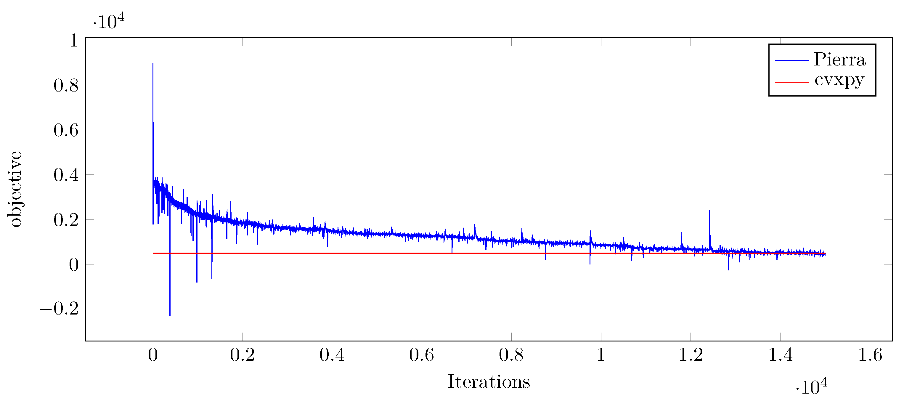
4.3. Numerical Results of Pierra’s Algorithm

This part shows the results of Pierra’s algorithm for Problem (19) in comparison with the solution of CVXPY for problem sizes $L\in \{3,4,\cdots ,10\}$. For these experiments, constant parameters are $\epsilon =1e-4$, $\lambda =0.5$, $k=3$, and $\alpha ={10}^{-8}$. $Z^1$ is chosen as $0_{(2m+4,2m+4)}$.

Table 2. Comparison between CVXPY and Pierra.

	Time (s)		Storage Needed (mB)
L	CVXPY	Pierra	CVXPY	Pierra	Optimality Percentage of Pierra (% CVXPY)
3	11	3.7	1.29792	0.13632	96.4%
4	49.6761	97.2	9.2	0.50496	77%
5	145.93	631	40.45	1.358848	86%
6	394.2456	1005.4	132.88	3.008448	92.2%
7	935.8	2275	358.82	5.841792	92.4%
8	2274.85	7826	841.73	10.32448	96%
9	4724.6	22338	1776.192	16.99968	97%
10	9244.87	63585	3451.17	26.488128	99.93%

shows the computation time and memory storage needed for both the computation using CVXPY and of Pierra’s algorithm, as well as the percentage of optimality of Pierra’s solution compared to CVXPY after about 10,000 iterations. The memory space saving is important. For $L=10$, the proposed algorithm reduced the memory consumption from 3.45 gigabytes to 26 megabytes: a factor of 100. In a reasonable computation time (that is, however, longer than the computation time of CVXPY), Pierra’s algorithm achieves great percentages from optimality. Figure 1 shows an example of the evolution of the objective function along the iterations of Pierra’s algorithm for the problem size $L=10$, compared to the optimal solution obtained by CVXPY. In this example, $P=\mathrm{15,000}$, and $\epsilon ={10}^{-4}$. A very good convergence can be observed at the last iterations shown in Table 2: $99.93\%$ from optimality.

4.4. Discussion

In conclusion of the numerical experiments, it is possible to make the following comments. The instance-based lower bounds obtained by using Pierra’s algorithm have been provided for small problem sizes. Thus, the contribution of this work is to propose a method to evaluate the solution of a heuristic algorithm for Problem (7) without comparing it with CPLEX, but rather with a lower bound. For this, a challenge has been encountered, because it is well known that using the duality makes the problems easier but bigger, as the dual problem is usually polynomial, but has more variables and more constraints. This challenge has been tackled by using Pierra’s algorithm with the sparse computations. Here, the goal is twofold: first, put the algorithm proposed by Pierra in 1984 back in the spotlight for its practical efficiency even if it has not been used much. The second goal is to show the power of having an explicit algorithm instead of a black box solver. Doing this has made the sparse computations possible, drastically reducing the need for memory storage. It would be interesting to compare the sparse version of Pierra’s algorithm with a sparse SDP solver such as the dual-scaling interior point algorithm [41].

Interesting future works involve going further in the problem sizes: starting from a grid of size $L=40$, the problem becomes computationally demanding, as CPLEX becomes unable of giving a solution, and CVXPY for the lower bound requires terabytes of memory storage. However, before this can be achieved, some challenges with Pierra’s algorithm need to be addressed, such as the stopping criteria on line 19 of Algorithm 3 and the performance of the algorithm that has to be sped up. One should note that the architecture of the algorithm allows a very easy parallelization, because the projections on each constraint space are independent (lines 6 to 17 of Algorithm 3). Thus, a parallel approach could speed up the algorithm.

5. Conclusions

This paper studies the robust counterpart of the shortest-path problem (RSPP) in the case of the correlated ellipsoidal uncertainty set. This problem is NP-hard, and exact methods exist to solve it, such as BSOCP solvers. Moreover, a heuristic algorithm named DFW has been proposed in [17]. In this paper, we propose a lower bound to validate heuristic approaches that solve the RSPP, such as DFW algorithm. This lower bound computation replaces the comparison with exact solvers as a validation method. To compute the proposed lower bound, recall that it is the solution of an SDP problem that can be solved by CVXPY by using interior-point methods. Unfortunately, the bidual problem is a big problem with many more constraints and more variables than the original problem. Thus, despite its polynomial nature, the resolution of this bidual problem is very time consuming and uses a huge memory space. Therefore, the sparsity of the matrices that define the problem has been exploited to replace the classical solver by a sparse version of Pierra’s decomposition through formalization in a product space algorithm. All this is numerically tested, showing that, due to the results of this paper, a polynomial time evaluation of the quality of the solution of the DFW heuristic is possible without having the memory storage issue of the bidual problem.

References

1. Kouvelis, P.; Yu, G. Robust Discrete Optimization and Its Applications; Springer Science & Business Media: New York, NY, USA, 2013; Volume 14. [Google Scholar]
2. Li, Z.; Ding, R.; Floudas, C.A. A comparative theoretical and computational study on robust counterpart optimization: I. Robust linear optimization and robust mixed integer linear optimization. Ind. Eng. Chem. Res. 2011, 50, 10567–10603. [Google Scholar] [CrossRef] [PubMed] [Green Version]
3. Ben-Tal, A.; Goryashko, A.; Guslitzer, E.; Nemirovski, A. Adjustable robust solutions of uncertain linear programs. Math. Program. 2004, 99, 351–376. [Google Scholar] [CrossRef]
4. Hanasusanto, G.A.; Kuhn, D.; Wiesemann, W. K-adaptability in two-stage distributionally robust binary programming. Oper. Res. Lett. 2016, 44, 6–11. [Google Scholar] [CrossRef] [Green Version]
5. Rahimian, H.; Mehrotra, S. Distributionally robust optimization: A review. arXiv 2019, arXiv:1908.05659. [Google Scholar]
6. Baron, O.; Berman, O.; Fazel-Zarandi, M.M.; Roshanaei, V. Almost Robust Discrete Optimization. Eur. J. Oper. Res. 2019, 276, 451–465. [Google Scholar] [CrossRef]
7. Buhmann, J.M.; Gronskiy, A.Y.; Mihalák, M.; Pröger, T.; Šrámek, R.; Widmayer, P. Robust optimization in the presence of uncertainty: A generic approach. J. Comput. Syst. Sci. 2018, 94, 135–166. [Google Scholar] [CrossRef]
8. Hazan, E. Introduction to online convex optimization. Found. Trends® Optim. 2016, 2, 157–325. [Google Scholar] [CrossRef] [Green Version]
9. Liu, B. Some research problems in uncertainty theory. J. Uncertain Syst. 2009, 3, 3–10. [Google Scholar]
10. Gao, Y. Shortest path problem with uncertain arc lengths. Comput. Math. Appl. 2011, 62, 2591–2600. [Google Scholar] [CrossRef] [Green Version]
11. Markowitz, H. Portfolio selection. J. Financ. 1952, 7, 77–91. [Google Scholar]
12. Poss, M. Robust combinatorial optimization with knapsack uncertainty. Discret. Optim. 2018, 27, 88–102. [Google Scholar] [CrossRef] [Green Version]
13. Nikolova, E. Approximation algorithms for reliable stochastic combinatorial optimization. In Approximation, Randomization, and Combinatorial Optimization. Algorithms and Techniques; Springer: Berlin/Heidelberg, Germany, 2010; pp. 338–351. [Google Scholar]
14. Baumann, F.; Buchheim, C.; Ilyina, A. A Lagrangean decomposition approach for robust combinatorial optimization. In Technical Report; Optimization Online; 2014; Available online: http://www.optimization-online.org/DB_FILE/2014/07/4471.pdf (accessed on 22 October 2019).
15. Atamtürk, A.; Narayanan, V. Polymatroids and mean-risk minimization in discrete optimization. Oper. Res. Lett. 2008, 36, 618–622. [Google Scholar] [CrossRef] [Green Version]
16. Buchheim, C.; Kurtz, J. Robust combinatorial optimization under convex and discrete cost uncertainty. EURO J. Comput. Optim. 2018, 6, 211–238. [Google Scholar] [CrossRef]
17. Al Dahik, C.; Al Masry, Z.; Chrétien, S.; Nicod, J.M.; Rabehasaina, L. A Frank-Wolfe Based Algorithm for Robust Discrete Optimization under Uncertainty. In Proceedings of the 2020 Prognostics and Health Management Conference (PHM-Besançon), Besançon, France, 4–7 May 2020; IEEE: New York, NY, USA, 2020; pp. 247–252. [Google Scholar]
18. Boyd, S.; Boyd, S.P.; Vandenberghe, L. Convex Optimization; Cambridge University Press: Cambridge, UK, 2004. [Google Scholar]
19. Anjos, M.F.; Lasserre, J.B. Handbook on Semidefinite, Conic and Polynomial Optimization; Springer Science & Business Media: New York, NY, USA, 2011; Volume 166. [Google Scholar]
20. Scobey, P.; Kabe, D. Vector quadratic programming problems and inequality constrained least squares estimation. J. Indust. Math. Soc. 1978, 28, 37–49. [Google Scholar]
21. Fletcher, R. A nonlinear programming problem in statistics (educational testing). SIAM J. Sci. Stat. Comput. 1981, 2, 257–267. [Google Scholar] [CrossRef]
22. Boyd, S.; El Ghaoui, L.; Feron, E.; Balakrishnan, V. Linear Matrix Inequalities in System and Control Theory; Siam: Philadelphia, PA, USA, 1994; Volume 15. [Google Scholar]
23. Goemans, M.X.; Williamson, D.P. Improved approximation algorithms for maximum cut and satisfiability problems using semidefinite programming. J. ACM (JACM) 1995, 42, 1115–1145. [Google Scholar] [CrossRef]
24. Karger, D.; Motwani, R.; Sudan, M. Approximate graph coloring by semidefinite programming. J. ACM (JACM) 1998, 45, 246–265. [Google Scholar] [CrossRef]
25. Goemans, M.X.; Williamson, D.P. New 34-approximation algorithms for the maximum satisfiability problem. SIAM J. Discret. Math. 1994, 7, 656–666. [Google Scholar] [CrossRef]
26. Lemaréchal, C.; Oustry, F. Semidefinite relaxations and Lagrangian duality with application to combinatorial optimization. Ph.D. Thesis, National Institute for Research in Digital Science and Technology (INRIA), Grenoble-Rhone-Alpes, France, 1999. [Google Scholar]
27. Goemans, M.X. Semidefinite programming in combinatorial optimization. Math. Program. 1997, 79, 143–161. [Google Scholar] [CrossRef]
28. Wolkowicz, H. Semidefinite and Lagrangian relaxations for hard combinatorial problems. In Proceedings of the IFIP Conference on System Modeling and Optimization, Cambridge, UK, 12–16 July 1999; Springer: Berlin/Heidelberg, Germany, 1999; pp. 269–309. [Google Scholar]
29. Nesterov, Y.; Nemirovski, A. Interior-Point Polynomial Algorithms in Convex Programming; Studies in Applied and Numerical Mathematics Series; Book Code AM13; Society for Industrial and Applied Mathematics: Philadelphia, PA, USA, 1994; pp. ix + 396. [Google Scholar]
30. Boyd, S.; Parikh, N.; Chu, E. Distributed Optimization and Statistical Learning Via the Alternating Direction Method of Multipliers; Now Publishers Inc.: Delft, The Netherlands, 2011. [Google Scholar]
31. Pierra, G. Decomposition through Formalization in a Product Space. Math. Program. 1984, 28, 96–115. [Google Scholar] [CrossRef]
32. Schrijver, A. A course in combinatorial optimization. CWI Kruislaan 2003, 413, 1098. [Google Scholar]
33. Chew, V. Confidence, prediction, and tolerance regions for the multivariate normal distribution. J. Am. Stat. Assoc. 1966, 61, 605–617. [Google Scholar] [CrossRef]
34. Ilyina, A. Combinatorial Optimization under Ellipsoidal Uncertainty. Ph.D. Thesis, Technische Universität Dortmund, Dortmund Germany, 2017. [Google Scholar]
35. IBM Academic Portal. Available online: https://www.ibm.com/academic (accessed on 22 October 2019).
36. Frank, M.; Wolfe, P. An algorithm for quadratic programming. Nav. Res. Logist. Q. 1956, 3, 95–110. [Google Scholar] [CrossRef]
37. Lee, J. A First Course in Combinatorial Optimization; Cambridge University Press: Cambridge, UK, 2004; Volume 36. [Google Scholar]
38. Diamond, S.; Boyd, S. CVXPY: A Python-embedded modeling language for convex optimization. J. Mach. Learn. Res. 2016, 17, 2909–2913. [Google Scholar]
39. Karloff, H. How Good is the Goemans–Williamson MAX CUT Algorithm? SIAM J. Comput. 1999, 29, 336–350. [Google Scholar] [CrossRef]
40. Dijkstra, E.W. A note on two problems in connexion with graphs. Numer. Math. 1959, 1, 269–271. [Google Scholar] [CrossRef]
41. Benson, S.J.; Ye, Y.; Zhang, X. Solving large-scale sparse semidefinite programs for combinatorial optimization. SIAM J. Optim. 2000, 10, 443–461. [Google Scholar] [CrossRef] [Green Version]
Figure 1. Evolution of the objective function along 15,000 iterations in Pierra’s algorithm compared to CVXPY’s solution for L = 10 .
Mathematics 10 04009 g001