Abstract
This paper addresses the robust job-shop scheduling problems (RJSSP) with stochastic deteriorating processing times by considering the resilience of the production schedule. To deal with the disturbances caused by the processing time variations, the expected deviation between the realized makespan and the initial makespan is adopted to measure the robustness of a schedule. A surrogate model for robust scheduling is proposed, which can optimize both the schedule performance and robustness of RJSSP. Specifically, the computational burden of simulation is considered a deficiency for robustness evaluation under the disturbance of stochastic processing times. Therefore, a resilience-based surrogate robustness measure (SRM-R) is provided for the robustness estimation in the surrogate model. The proposed SRM-R considers the production resilience and can utilize the available information on stochastic deteriorating processing times and slack times in the schedule structure by analyzing the disturbance propagation of the correlated operations in the schedule. Finally, a multi-objective hybrid estimation of distribution algorithm is employed to obtain the Pareto optimal solutions of RJSSP. The simulation experiment results show that the presented SRM-R is effective and can provide the Pareto solutions with a lower computational burden. Furthermore, an RJSSP case derived from the manufacturing environment demonstrates that the proposed approach can generate satisfactory robust solutions with significantly improved computational efficiency.
Keywords:
production resilience; robust job-shop scheduling; surrogate robustness measure; disturbance propagation; optimization algorithm MSC:
90B36
1. Introduction
Scheduling problems always play a key role in improving the production efficiency of a manufacturing system, such as flow shop scheduling [1,2], job-shop scheduling [3,4], and flexible job-shop scheduling [5,6,7]. The job shop is a typical workshop organization form to model the manufacturing environment. In recent years, tremendous research work has been conducted by considering a deterministic environment [8]. However, in a real-life job shop, the processing times would be deteriorated by many uncertainties, such as random machine breakdowns, uncertain setup times, and the unavailability of fixtures [9,10,11]. For example, in the aero-engine parts workshop, machine failures will cause processing interruption, and thus extend the processing time, or the tool wear will increase the actual processing time. Since the random deterioration of the processing time may decrease the production performance of a real-life manufacturing system, how to effectively deal with the job-shop scheduling problem (JSSP) with it has become a critical and interesting issue. There are four major approaches for dealing with such problems: a stochastic approach, a fuzzy approach, a stability approach, and a robust approach [12]. The stochastic approach [13] assumed that the job processing times are random variables with certain probability distributions determined before scheduling. A fuzzy approach [14] allows a scheduler to find the best schedules, with respect to the fuzzy processing times of the jobs to be processed. The stability approach was developed to construct a minimal dominant set of schedules, which optimally covers all feasible scenarios. For example, Sotskov et al. [15] addressed a two-machine job-shop scheduling problem with fixed lower and upper bounds on the job processing times and provided a minimal dominant set of schedules to make the online scheduling decision. A robust approach considers the robustness to generate a schedule that can preserve a specified level of solution quality in the presence of uncertainties [16]. Generally, robustness has two definitions: quality robustness and solution robustness [17]. Quality robustness is used to indicate the insensitivity of the schedule performance under uncertainties, such as makespan or tardiness. The solution robustness refers to the insensitivity of activity start times to uncertainty [7,18]. In this study, we will focus on the quality robustness to deal with the robust job-shop scheduling problems.
For quality robustness, some studies used the minimized maximum regret value to evaluate it [8] and some regard the expected actual performance as the robustness [4,19]. For example, Wu et al. [20] proposed a decomposition method based on graph theory for JSSP, by using expected average weighted tardiness as a robustness measure. However, taking the expected performance as the robustness evaluation measure cannot evaluate the degree of influence of disturbances on the scheduling performance. To address this, the Pareto optimization method can be applied to optimize scheduling performance and robustness at the same time, just like when Xiong et al. [7] studied the flexible job-shop dual-objective robust scheduling problem with random machine failures. However, a new problem is that the robustness measure cannot be calculated analytically for the job-shop scheduling.
Robust scheduling based on simulation evaluation is an effective method [8], which can use the Monte Carlo simulation to simulate stochastic processing times to evaluate the robustness approximately. However, for a large number of processing time scenarios that are required to get a reasonable approximation, this type of method often bears an unacceptable computational burden [6,21]. By comparison, using the surrogate robustness measure (SRM) is an effective method to improve the computational efficiency of robustness evaluation [22,23]. In essence, the SRM is an approximate estimation measure that uses the partially known information of random disturbances and the structure of the schedule to decrease the computational burden of the robustness evaluation [13,24].
In recent years, researchers have begun to apply the surrogate model based on a surrogate measure to scheduling problems under the influence of uncertainties. Zahid et al. [25] investigated the surrogate measure of robustness for project scheduling problems. The authors stated that to avoid large tardiness due to disturbances, managers might opt for a more robust schedule rather than an optimal schedule. Therefore, they emphasized the importance of the SRMs that aid in identifying proactive schedules, which can provide flexible yet efficient plans with minimum redundancy. Wu et al. [26] address the optimization of risks in performance and stability (solution robustness) for the job-shop scheduling under random machine breakdowns. They considered three objectives: makespan, makespan risk, and stability risk. Then, they used the buffering approach under the limited predictive makespan to generate predictive schedules, which allows inserting additional idle time to control the risks. Zheng et al. [27] studied the production scheduling problem in an assembly manufacturing system with uncertain processing time and random machine breakdown. They considered the objectives of minimizing makespan and the performance deviation of the actual schedule from the baseline schedule. Xiong et al. [7] suggested two surrogate measures for the flexible job-shop scheduling problem with random machine breakdowns, considering both the available uncertainty information and the schedule structure. Yang et al. [28] studied a flexible job-shop schedule problem (FJSP) with random machine breakdown. They considered the makespan and robustness as the scheduling objectives. Then, they developed one surrogate measure named RMc to evaluate robustness using the heuristics of maximizing the workload and float time of each operation and the machine breakdowns.
From the above literature, although great efforts have been conducted for the robust scheduling problems in the field of production scheduling and project scheduling, a further study is urgently needed to consider the resilience of the manufacturing system to construct a more accurate surrogate robustness measure. System resilience is the ability of a system to respond and recover quickly from an external disruptive event [29]. In recent years, studies have been conducted considering system resilience. Mao et al. [30] formulates the supply chain networks problem as a network maximum-resilience decision, and thus developed the resilience of cumulative performance loss and the resilience of restoration rapidity to measure the resilience of the supply chain networks. Dui et al. [29] studied data-driven maintenance priority and resilience evaluation of performance loss in the main coolant system, in which the resilience of the MCS is represented by the loss and recovery of system performance. To effectively reduce and prevent losses, a resilience importance measure for performance loss is proposed to evaluate the performance of the main coolant system. Qi et al. [31] proposed a metro network’s robustness and vulnerability measurement method under node interruption and edge failure based on the complex network modeling and topological characteristics analysis of metro systems. Robustness is an important connotation of system resilience; therefore, it has the potential to design better surrogate robustness measures based on resilience.
In the previous study, the authors made some contributions in the field of job-shop scheduling under uncertainties. The authors have considered the methods of robust scheduling and risk control to deal with the disturbances to improve the robustness and reduce the scheduling risk of the job shop. Xiao et al. [22] proposed an effective robustness surrogate measure for the job-shop scheduling problem with stochastic processing time and a hybrid estimation of the distribution algorithm. Wu et al. [23,24,26] studied the job-shop scheduling problem under random machine failures and proposed robust and/or stability optimization methods based on risk indicators. To further solve the JSSP under machine–worker dual resource constraints, Xiao et al. [32] proposed a multi-objective hybrid distribution estimation algorithm (MO-HEDA). At the same time, Dui et al. [29] carried out extended research in the field of system resilience and reliability. Although the existing research has made some progress, the robustness evaluation accuracy and the solution efficiency for solving the RJSSP are still restricted by uncertainties. This study focuses on the RJSSP under stochastic deteriorating processing times, which are assumed to follow the truncated normal distribution. The main contributions can be attributed as follows. First, we constructed a surrogate model of robust scheduling, considering the performance and the robustness at the same time, in which the robustness is evaluated by a surrogate robustness measure. Second, we proposed a new effective resilience-based surrogate robustness measure (SRM-R) that considers the disturbance propagation process. Moreover, we adopt a multi-objective hybrid estimation of the distribution algorithm (MO-HEDA) based on the research of Xiao et al. [18], which can provide the Pareto optimal solutions with a satisfactory performance by minimizing the SRM-R and the performance measure simultaneously.
The organization of this paper is as follows. Section 2 provides the problem description and the mathematical modeling of RJSSP. Section 3 investigates the existing SRMs and then presents an SRM based on the resilience and disturbance propagation among the operations. Section 4 provided the MO-HEDA for the dual-objective RJSSP. Section 5 verifies the effectiveness and performance of the presented SRM-R for bi-objective robust scheduling by three groups of computational experiments. Moreover, we show the effectiveness of the proposed surrogate model by using a scheduling problem instance derived from a real-life manufacturing workshop. Finally, we draw some conclusions and provide directions for future research in Section 6.
2. Problem Description and Surrogate Model
2.1. Problem Description
The notations that are used in the formulation of the RJSSP are defined in Table 1.

Table 1.
The notations of the mathematical model.
In the literature on stochastic scheduling, various types of probability distributions for stochastic processing times have been studied, such as exponential distribution, normal distribution, and uniform distribution. One method is to treat both the stochastic processing time and the scheduling objective as the stochastic variables, which aims at providing the processing ordering of the tasks on the machines with an expected optimization model. The historical processing data can be collected and used to get the probability distribution. To model the uncertain processing time, the actual job processing time is usually generated from a normal distribution with its expected value and the standard deviation, such as Gu et al. [19], Horng et al. [4], Wang et al. [13,33]. Therefore, the normal distribution is a representative type to study the stochastic processing times in the field of job-shop scheduling with uncertainty.
The RJSSP based on a classic job-shop scheduling problem is described as follows: jobs processed on machines; each job has operations. The probability distribution of the stochastic processing times is derived from the historical manufacturing data. In this study, all the stochastic processing times, are assumed to follow the normal distribution, i.e., , where denotes the value of deteriorating disturbances on the expected processing time scenario. The processing information of any operation is denoted as a vector . Let denotes the feasible solution set that meets the process constraints. A feasible schedule is denoted by .
In an arbitrary schedule, the expected processing time is a nominal value, then the total start time deviation of each operation is affected by two factors. The first factor is the internal disruption that occurs in the operation . The second factor is the unabsorbed deviation caused by the preceding job on the same machine or by the preceding machine of the job . We use Figure 1 to explain how the deviation in operatn . is caused.
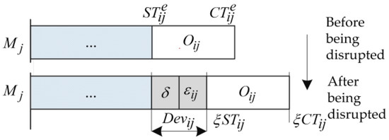
Figure 1.
The start time deviation after being disrupted.
Figure 1 shows the deviation of the start time of the operation caused by the disruption of the machine . Before the disruption occurs, the start time and completion time of are denoted by and , respectively. After the disruption occurs, the estimated start time and completion time are denoted by and , respectively. Thus, the total deviation of start time is indicated by , where denotes the disruption caused by the preceding operation of the same job or the preceding job on the same machine.
2.2. Mathematical Formulation of the Surrogate Model
We use the Pareto optimization method to perform robust scheduling, thus, providing decision makers with a set of Pareto solutions that meet different risk preferences. The surrogate model of RJSSP is described as by a triplet proposed by Graham et al. [34], where denotes the JSSP, SPT denotes the stochastic deteriorating processing times, and and are the objectives that need to be optimized. Specifically, the SRM is used to evaluate the robustness of a schedule. The mathematical model of RJSSP is shown as follows:
s.t.
The objective functions are shown in Equation (1). The predictive makespan of a schedule is obtained by using the expected values of the processing times by function . Function is used to evaluate the robustness of a schedule solution. Inequality (4) represents the process constraints, which means the job must be processed on the machine before being processed on the machine . is a large enough positive number. The machine constraints are denoted by inequality (5), which means the job must be processed on the machine after job . Constraints (6) and (7) denote one machine can only process one job at one time and one job can only be processed on one machine at the same time. Constraints (8) and (9) represent the value of and can only be the integers 1 or 0. Inequality (10) denotes that none of the completion times of the operations can be negative.
3. The SRM-R for the Surrogate Model
Robust scheduling aims to generate the initial schedule with a satisfactory makespan and be capable of absorbing the disturbances caused by the deteriorating processing times when a right-shift reaction policy is adopted [35]. Generally, the robustness is estimated through Monte Carlo simulation by generating a certain number of processing times scenarios, which can be calculated by the following function:
where denotes the number of simulation replications, denotes the simulation-based robustness, denotes the makespan of schedule under the processing time scenario. In this paper, the processing time scenario indicates a group of potentially realized stochastic deteriorating processing times of all the operations.
The simulation-based robustness evaluation is time- and resource-intensive. Thus, the robustness of a schedule is usually evaluated by designing an SRM to avoid the computational burden caused by simulations. However, in the previous research, seldom effective SRM for RJSSP have been developed. We analyze five typical existing SRMs and then propose an SRM for RJSSP by using a statistical method and a disturbance propagation formula.
3.1. The Existing Surrogate Robustness Measures
In the research of Leon et al. [35], an SRM for evaluating the absorption capability of a schedule was proposed based on the average total slacks. The measure is rewritten as SRM1, where denotes the total slack time of the operation .
The SRMs that aim at providing an estimation of the schedule robustness for multi-mode project scheduling problems were investigated by Hazir et al. [36]. In one robustness measure, they define the activities that have the total slacks less than , of the activity duration as the potentially critical activities (PCA), i.e., . The delays in PCA are likely to result in delays in the project completion time. Thus, those schedules with fewer critical activities are preferred on the robustness. The measure of PCA used in RJSSP is reasonable because of the similarity of the two problems, which is renamed potential critical operations (PCO). Considering the variance of RJSSP is assumed known, the definition of PCA is revised as the ratio of total slacks and the sum of planned processing time and standard deviation, i.e., . Therefore, the SRM is rewritten as follows:
where denotes the number of PCOs, denotes the set of PCO, which includes all the operations that satisfy the inequality .
Goren et al. [37] developed a surrogate stability measure to generate efficient and stable schedules for a job-shop subject to processing time variability and random machine breakdowns. The SRM is based on decreasing the maximum variance on the mean critical path, where the mean critical path is equivalent to the critical path of RJSSP when expected processing times are used. The SRM is written as follows:
where the objective of SRM3 is to evaluate and select the critical path with the maximum sum variances, in which VAR denotes the variance of the processing times of the operations in the critical operation .
Xiao et al. [22] provided two SRMs for the robust scheduling of JSSP with stochastic processing times. They utilize the probability distribution information of stochastic processing times and the structure of the schedule solution determined by the slack times to estimate the robustness.
In Equation (15), and denote the estimated robustness degradation of the critical path and the non-critical path, respectively. The aims to minimize the total robustness degradation of the baseline schedule.
In Equation (16), is provided to estimate the possible robustness degradation by minimizing the maximal robustness degradation on the critical path and non-critical path. In the following section, a disturbance propagation-based SRM is proposed, which is inspired by the disturbance absorption ability of a baseline schedule.
3.2. The Resilience-Based Surrogate Robustness Measures
One of the core connotations of system resilience is the ability to absorb disturbances, which is reflected by the degree of system performance degradation under disturbance events. From this point of view, a schedule with good resilience may also have strong robustness. Therefore, we constructed a resilience-based surrogate robustness measure by analyzing the influence and propagation mechanism of stochastic deteriorating processing times to the makespan.
To describe the realized processing time scenario, the stochastic deteriorating disturbances were represented by when disruption was introduced. In this study, the processing times of each operation are considered to follow a normal distribution, i.e., . Then, map into , yielding . Furthermore, was denoted as the confidence level that is specified by the decision maker, considering the degree of risk aversion on the stochastic deteriorating processing times. We used the maximum possible value of the disruption with a certain confidence level to convert the disruption into a confidence interval. Then, the worst case of the disruption was utilized for designing the SRM for robustness estimation. Since we are concerned about the upper limit of the realized processing time, the right-sided confidence interval of the normal distribution function was used. The probability is represented by Equation (17),
where the value of realized processing time , is the critical value determined by the predefined value of . Therefore, the possible disturbance of operation follows the equation .
Since the disruptions among the operations propagate downstream under the process constraints, the recursion formula for calculating the of operation should be provided. Since the maximum value of the internal disruption is set by using a predefined confidence level consideration is required for the worst case of all the processing time scenarios. The scenarios denote the realization of the stochastic processing time of the operations. The main difficulty, thereby, is to analyze the disturbances caused by the preceding operations. We use a problem instance with two consecutive jobs and two machines to analyze how to estimate the total deviation of an arbitrary operation, as shown in Figure 2.
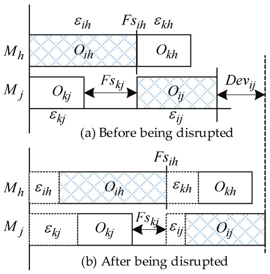
Figure 2.
An instance of two consecutive jobs processed on two machines.
We used Figure 2 to illustrate the schedule before and after the disruptions occur; denoted the possible maximum of the disruption of each operation; and denoted the free slacks of operation and , respectively, where . Generally, the absorption ability of the schedule is determined by the free slacks that exist in the schedule. To estimate the robustness of a schedule, we analyzed the formula of each operation first and then extended the formula into a generic form. Furthermore, the generalized formula for estimating the deviation was used to develop the SRM for estimating the robustness of RJSSP.
The operation and are in the first position on the machine and . The deviation and are represented by and , respectively. The deviation of operation is possibly affected by its preceding operation or beside the disruption . It was also found that there are some units of slack times before the operation , which can be regarded as the free slacks belonging to the operation . If , the free slacks cannot absorb the disruption of operation , otherwise, the deviation of operation will not influence the starting time of operation . In addition, the deviation of operation may also affect the deviation of operation , since its free slack is . Therefore, the total deviation was determined by the maximum deviation of its preceding job or operation. The available free slack is calculated by using the start time of and the maximum of the end time of operation and . From the above analysis, the is formulated as follows:
where and denoted the start time and completion time of the initial schedule, which are obtained by decoding the schedule using the nominal processing times . The reasonability lies in that the start times and completion times of the succeeding operation are shifted backward due to the adoption of the right-shift rescheduling method when disruption occurs. Therefore, the deviation of operation can be estimated by the following equation:
To generalize the formula for estimating the deviation on the arbitrary operation , we define as the preceding operation of the operation on the same machine and define as the preceding operation of the same job . There are two cases in which operation has no preceding operation or has no preceding job. The first case is that the operation is the first operation on a machine while the second one is that is the first operation of the job . To create a generic formula, four cases were discussed by considering whether the operation is the first operation on a machine and whether operation is the first operation of the job . We used to represent the job on the machine and used to denote the operation of job . Therefore, the deviation of the operation that considers the disturbance propagation was calculated by the following equation:
where indicates that the first operation on the machine is while indicates that is the first operation of Job . Due to the adoption of the railway execution strategy, the start time of cannot move forward, then the deviation of any operation cannot be negative. Moreover, the difference between the deviation and the free slack should be greater or equal to zero in the case that the disruption is fully absorbed. To further simplify the formula for estimating , we provide the following Proposition 1.
Proposition 1.
For in the schedule , if the operation has at least one preceding job or one preceding operation, it holds that at least one of the two inequalities between and are satisfied in any case.
Proof of Proposition 1.
For , the following four cases cover all the possibilities:
- Case 1, if , there is no preceding operation and preceding job before the operation , it is easy to find that ;
- Case 2, Else if , there is at least one operation that precedes of job , then ;
- Case 3, Else if , there is at least one operation precedes on the machine , then ;
- Case 4, Otherwise, , there exists at least one operation that precedes of job and at least one operation precedes on the machine , then . It can be seen from the four cases that if an operation has no preceding jobs and preceding operations, its start time is equal to zero.
In other cases, there are at least one of the two equations of and holds. Since it also holds that and , therefore, at least one inequality in and is satisfied in any case.□
According to Proposition 1, the formula in Equation (20) is rewritten as Equation (21)
By Equation (21), the completion time of each operation after being disrupted is estimated by Equation (22).
According to Equation (22), the makespan is calculated by Equation (23).
In Equation (23), , and the estimated disruption in the formula of can be deemed as constants. Thereby, the only unknown parameter is the disturbance caused by the adjacent preceding operations and the available free slack times. For each schedule solution , the estimated deviation of the makespan is calculated by Equation (24):
where denotes the estimated deviation between the makespan after the disruptions and the initial makespan, considering the nominal processing times.
To keep the higher robustness of a schedule , the should be minimized. Therefore, the presented SRM is written as Equation (25):
where SRM-R denotes the proposed SRM. Therefore, the schedule with a higher disruption absorption capability, which keeps a lower deviation of the makespan, was selected.
4. A Dual-Objective Optimization Algorithm
The estimation of distribution algorithm (EDA) is an evolutionary algorithm that explores the space of candidate solutions by using an explicit probabilistic model [38]. In this study, the procedures of HEDA presented by Xiao et al. [22,32,39] are adopted as the basis of MO-HEDA for solving the surrogate model of RJSSP.
In this section, an improved multi-objective optimization algorithm based on the HEDA is adopted [32]. Before describing the MO-HEDA, the definitions are described:
Definition 1.
Pareto optimal solution: A schedule solution
is Pareto optimal solution if there is no other solution
that dominates
.
Definition 2.
Pareto front: The Pareto front denotes the Pareto boundary constructed by the Pareto optimal solutions.
Definition 3.
Dominance: For
, there exist M objectives
for each solution. It is said that
dominates
, if and only if
, and there exists at least one
satisfied
.
The MO-HEDA is developed by combining the HEDA and NSGA-II [40,41]. The framework of the MO-HEDA is shown in Figure 3.
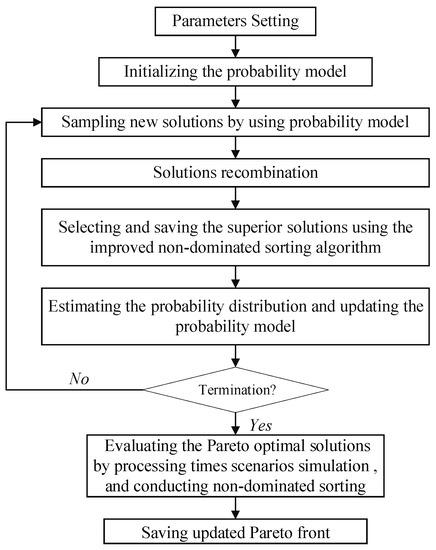
Figure 3.
The framework of the MO-HEDA.
In the first three steps, the algorithm is used to get the Pareto optimal solution by running given generations. When RMsim is used as the robustness measure, simulation-based evaluation is adopted in the evolutionary process, then the Pareto front can be obtained directly. Then, the Pareto front will be further evaluated by Step 4 when SRM is used as the robustness measure. After being evaluated by simulation, the values of SRMs are turned into simulation-based robustness, which can be compared with the robustness obtained by simulation-based robustness. The pseudocode of MO-HEDA is shown in Algorithm 1.
| Algorithm 1. The pseudocode of MO-HEDA. |
| Step 1. Set the parameters: population size , the number of parents and offsprings , , the number of superior solutions , evolutionary generation , recombination probability , inheriting rate , learning rate . Step 2. Initialize the algorithm. Step 2.1 Generate , initial schedule solutions, let denote the initial solution set, is the index of iteration. Step 2.2 Decode the solution to obtain the fitness value of each objective ; denotes the number of objectives. Step 2.3 Calculate the probability matrix . Step 3. Set While Do Step 3.1 1 Generate new solutions by using the probability matrix . Let denote the newly generated solution set. Step 3.2 Merge the solution set and to get a new solution set . Step 3.2.1 Execute the improved non-dominated sort algorithm to obtain the non-dominated levels of the Pareto solutions. Let denote the solution set in all the non-dominated levels, where denotes the first level. Step 3.2.2 Set While Do Else if , the solutions are selected by using the crowded-comparison operator; End While Step 3.2.3 Sort the solutions in the new solution set . Step 3.3 Select the first solutions in as the parent solutions. Step 3.4 Generate offspring solutions by using the recombination method with the recombination probability and then sort the solutions by using the same procedure as Step 3.2 to obtain an updated solution set . Step 3.5 Select superior solution to update the probability matrix of HEDA and save elites in the solution set or the next iteration by using the crowded-comparison operator. ; End While Step 4. Robustness evaluation by Monte Carlo simulation method. Step 4.1 Conduct the simulation evaluation on the obtained Pareto optimal solutions in the solution set . Step 4.2 Sort the solutions in according to the simulation results by using the improved non-dominated sort algorithm. Step 4.3 Save the Pareto frontier of the simulated solutions. |
In the MO-HEDA, we used an operation-based encoding scheme [22]. Each in the population denotes a scheduling solution of the RJSSP. The operations of the job are represented by . Let , where denotes the positions in each solution. Under the encoding scheme, in the position of in denotes that the operation of the job is located at the position of . The individual will never produce infeasible solutions in both the population initialization process and the individual sampling process, since it is encoded under precedence constraints.
The probability model is a vital procedure for the learning process of HEDA. The offspring solutions in each generation are produced by sampling the probability model. A probability matrix was defined considering the encoding scheme of RJSSP, where the element represents the probability of the operation on the machine of a job located in the position . The probability function of the superior population is written as Equation (26):
where denotes the quantity of the superior population, denotes the statistical function, according to Equation (27):
To update the probability matrix of each generation, an incremental learning rule in the field of machine learning was adopted. The learning function is shown in Equation (28).
The recombination method of HEDA is designed considering the encoding scheme and the requirement of inheriting the excellent structure of the parent solutions [13,22]. With the recombination scheme, feasible solutions are generated directly and do not need a repairing process. As described by Xiao et al. [39], HEDA adopts an operation-based individual recombination method. This operator relies on the parent’s operation inheritance rate, which represents the number of jobs that need to be inherited from the relative position and is used to adjust the inheritance degree of the offspring to the parent’s structural characteristics. To perform the recombination process, we first set the value of the parent process inheritance rate and the recombination probability; second, we selected μ parent individuals and N positioning jobs, and found the positioning operations of jobs and the relative positions of the parent individuals, named P1 and P2, respectively. At last, we extracted all the operations of the remaining jobs, inserted the remaining operations of P1 into the vacancy of the offspring S2 in sequence, and inserted the remaining operations of P2 into the vacancy of the offspring S1 in sequence.
The non-dominated sort algorithm is an innovative algorithm for sorting a population into different non-domination levels. However, the algorithm can be further improved by reducing the storage space complexity of the solutions and the number of comparisons in the sorting process. The computational complexity of the non-dominated sort algorithm is , where denotes the number of objectives and N denotes the size of the population. As stated by Deb et al. [40], although the computational time complexity has reduced to , the storage requirement has increased to . Therefore, there are two aspects of the previous algorithm that can be further improved. First, the comparison of each solution is conducted twice. Second, the solution set is dominated by the arbitrary solution will be stored in the cache, while the dominated set will not be outputted. Therefore, the improved non-dominated sort algorithm is adopted. The procedures are shown in Algorithm 2.
| Algorithm 2. The pseudocode of the improved non-dominated sort algorithm. |
| Step 1. Set the index of the solutions in the solution set , for each solution, set as the number that is dominated. Step 2. Determine the number that is dominated for each solution. For For If dominates ; Else if dominates ; End End Step 3. Sorting and storing the solutions in each front by using the times to be dominated. Step 3.1 Sorting the solutions based on the values of in ascending order. Step 3.2 For Set , denotes the number of solutions in each level. Set , is the index of the non-dominated level. If ; ; Else if ; ; End End Step 4. Return the solution sets . |
The overall complexity of the NSGA-II is , which is governed by the non-dominated sorting algorithm. The improved non-dominated sorting algorithm reduces the storage space complexity from to by adopting the above well-designed algorithm structure. Meanwhile, the time complexity of comparisons is reduced to from due to the solution comparison being reduced to once for each solution [32].
In the improved non-dominated sort algorithm, the niche selection technology is provided to maintain the diversity of Pareto solutions. In this way, the algorithm can converge to the uniformly distributed Pareto front. In this study, the crowding-distance assignment proposed by Deb et al. [40] is used. They defined density estimation to get an estimation of the density of solutions surrounding a particular solution in the solution set. The crowding distance is represented by the parameter of the cuboid formed by using the nearest neighbors as the vertices. For the arbitrary non-dominated solution set , the crowding distance of each solution can be calculated by the algorithm in Algorithm 3.
| Algorithm 3. The crowding distance assignment. |
| Step 1. Let Step 2. For Set For , sort the objective in an ascending order Set For End End End Step 3. Save the for the crowded-comparison operator. |
In the algorithm of crowding distance assignment, denotes the crowding distance of the objective of the solution , and represents the maximum and minimum of the objective in solution set . By using the algorithm 2 and algorithm 3, we obtained two attributes of the solution, i.e., the non-domination rank and crowding distance .
5. Simulation and Analysis
5.1. Experiment Setting
The experimental analysis approach and the MO-HEDA are both coded by Matlab 2016 on a computer of Intel(R) Xeon(R) CPU E31230 @ 3.2 GHz with RAM of 8.00 GB, produced by Dell, Round Rock, Texas. The parameters of MO-HEDA set the same values for both RMsim and SRM, which are listed in Table 2.
Table 2.
The parameters setting for MO-HEDA.
The benchmark instances are modified from the classic JSSP benchmark instances by introducing the variance into the nominal processing times. The benchmark instances of FT06, FT10, and FT20 provided by Muth and Thompson [42] and LA06, LA16, LA21, LA26, and LA32 provided by Lawrence [43] are selected.
5.2. The Effectiveness Analysis of SRM-R
This section focuses on the correlation analysis between the SRMs and the RMsim by using the coefficient of determination ( value). To analyze the values under different degrees of uncertainty, we define the terminology of uncertainty level.
Definition 4.
Uncertainty level (UL): The uncertain level denotes the corresponding degrees of uncertaintyin aRJSSPproblem instance, which is measured by the percentage of uncertain operationsrelative toall the operations.
The uncertain operations are selected randomly by a uniform distribution according to the specified UL. We choose five ULs (ULx, x = 2, 4, 6, 8, 10) to compare the correlation between the SRMs and the corresponding simulation-based robustness (RMsim). The value of RMsim is also calculated using Equation (11).
The compared SRMs are optimized without considering the makespan. The critical value for possible maximal processing time disruption is set at with a confidence level of 97.5%. The values are obtained from the regression of the values of SRM and the corresponding SRMsim in the optimization process of HEDA with 200 generations. For each benchmark, five existing SRMs [22] and the presented SRM-R are tested. The average values obtained by running HEDA ten times are shown in Table 3. Moreover, the average R2 values for all the selected ULs are provided to show the overall correlation of the comparison SRMs.
Table 3.
The value of the comparison SRMs.
5.3. The Performance Analysis of the Pareto Optimal Solutions
In this section, two different degrees of uncertainties are investigated by defining the benchmarks with 50% and 100% uncertain jobs as UL-M and UL-H, respectively, where UL-M denotes the medium uncertainty level and UL-H denotes the highest UL. To keep the benchmarks consistent when conducting robust scheduling by using SRM4 and RMsim, we select all the operations of the first [] jobs in each benchmark as the uncertain operations under UL-M, while all the operations of the n jobs will be selected as the uncertain operations under UL-H.
The simulation-based robustness measure is always regarded as the best one while with the largest computational burden [6,7]. Generally, the comparison is based on the set coverage between the Pareto front obtained by RMsim and that obtained by the proposed SRMs. In this study, we compare the performance of the presented SRM4 and RMsim directly, since the correlation values of the existing SRMs are apparently worse than those of the presented SRM4. To obtain the Pareto optimal solutions, the objective combinations of [makespan, RMsim] and [makespan, SRM-R] are used as the scheduling objectives. Two performance criteria are selected to conduct the performance comparison of RMsim and the presented SRM-R refers to the literature [7,44].
Set Coverage (SC): Let A and B be two Pareto solution sets, the set coverage SC (A, B) is defined as the percentage of the solutions in set B and is dominated by at least one solution in Pareto solution set A, as shown in Equation (29).
A higher value of indicates a better performance of set A. Referring to the study of Xiong et al. (2013) [7], we use SC1 and SC2 to indicate the set coverage of the two non-dominated sets obtained by the robustness measures RMsim and SRM-R. For the convenience of comparing the performance of SRM-R and RMsim, we define , .
Computational time (CT): The computational time of running the MO-HEDA on the same benchmark instance by using RMsim and SRM-R.
Moreover, to show that a certain number of Pareto solutions can be obtained by using the proposed surrogate robustness measure, the number of Pareto optimal solutions is defined. Since RJSSP is an NP-hard problem and the exact optimal solution can hardly be obtained, the mentioned Pareto optimal solution is not the exact Pareto optimal solution. Given this, we use the optimal solutions obtained by MO-HEDA as the Pareto optimal solutions.
The number of Pareto optimal solutions (NPS): the number of Pareto optimal solutions on the Pareto front in the last generation.
For each benchmark, the solution performance obtained by SRM-R and RMsim will be compared using the above performance metrics; those with better performance are marked in bold. The RJSSP is a complex NP-hard combinatorial optimization problem. Moreover, the stochastic processing times also increase the randomness of the Pareto optimal solutions. Therefore, the MO-HEDA usually cannot get the same Pareto front over different runs of MO-HEDA. In the simulation, we find that the Pareto optimal solutions over different runs of MO-HEDA converge to nearly the same Pareto front under small-size benchmarks. However, under large-size benchmark instances, the Pareto optimal solutions are hard to converge to the same Pareto front due to the randomness of the optimal solutions of MO-HEDA and the effects of stochastic processing times.
From Table 4, we find that the average NPS obtained by RMsim is slightly greater than that of SRM-R under both UL-M and UL-H. The reason lies in that the SRM-R, which is an estimator of RMsim, would be slightly worse than RMsim. Moreover, the robustness evaluation in Step 4 of the MO-HEDA will also decrease the NPS in the first Pareto front. Meanwhile, the average, as well as the difference of the average under UL-H, are less than that under UL-M, which demonstrates under higher UL, the optimal Pareto solutions are harder to be obtained due to the variability of the objective values under uncertain processing times. When compared with the average NPS over all the benchmarks, the NPS of SRM-R is smaller than that of RMsim, although the difference between the average NPS values under UL-H is slight.
Table 4.
The value of NPS.
The performance of the Pareto optimal solutions obtained by SRM-R and RMsim is represented by set coverage, shown in Table 5. Under the UL-M for the nine benchmarks, the values of SC2 range from 0.66 to 0.98; the SRM-R shows better optimal performance in two benchmarks. The average values of SC1 and SC2 over all the benchmarks are 0.78 and 0.9, respectively. It means there is about a 12% performance deviation of the Pareto solutions obtained by SRM-R and those obtained by RMsim under UL-M from an overall perspective. As seen from the results under UL-H, there are four benchmarks that show the better performance of SRM-R, which is 44.4% of the total number of the tested benchmarks. Moreover, the average value of SC2 is 0.79, which is very close to the value of SC1, namely, 0.84. In this study, the direct comparison of the set coverage between RMsim and SRM-R shows that a higher SC2 is obtained, which is ranging from 0.62 to 1.0. This result is very satisfying when compared with the performance of the SRM proposed for flexible JSSP by Xiong et al. [7], which is rarely greater than 0.2 over the tested problems. Therefore, it is concluded that Pareto solutions can be obtained by using SRM-R as an estimator of robustness.
Table 5.
The SC of the Pareto optimal solutions obtained by RMsim and SRM-R.
The main advantage of the SRM-R is the computational efficiency. The percentage of the decreasing of the CT of SRM-R, compared with that of RMsim is calculated by Equation (30).
The average of the CT of ten replications, as well as the relative percentage deviation under both the UL-M and UL-H over the nine benchmarks are provided in Table 6.
Table 6.
The comparison of average computational time (seconds).
It is easily found that the CT of SRM-R is significantly lower than that of RMsim. The decreasing percentage of CT ranges from 65.45% to 77.51% under UL-M and ranges from 66.82% to 78.46% under UL-H. The results are obtained with simulation replications of 50.
According to the analysis, it is verified that the presented SRM-R can estimate robustness accurately. Therefore, the decision makers can obtain the Pareto optimal solutions using SRM-R as the robustness measure with a tremendously lower computational time. Meanwhile, the RMsim is preferred when there is enough simulation time or more Pareto solutions are needed, since it can provide more Pareto solutions. However, if the decision makers want to obtain the Pareto solutions with high computational efficiency, especially for large-size problem instances, the presented SRM-R is a better choice.
5.4. Case Study
A typical problem instance derived from a job-shop manufacturing environment is selected [13]. The problem instance is extracted from the manufacturing enterprise and then modified to verify the effectiveness of the surrogate model for RJSSP. There are eight parts to be processed, which are typical aircraft engine parts. Each part requires six major processes, including turning, milling, planning, grinding, drilling, and boring. After the setup process of the machine tool is finished, it will then be machined by the machine tool automatically. The machine tools are numbered, respectively, including lathe (M1), milling machine (M2), planer (M3), grinding machine (M4), drilling machine (M5), and boring machine (M6). The sample mean and variance of the processing time of each process are obtained, according to the historical data. The processing times approximately follow the normal distribution, then the processing time scenarios are assumed to follow the trunked normal distribution. The corresponding machine information and processing time information (units/hour) are shown in the form of (the machine number, the expected value, and the variance) [13]. We solve the problem instance using the surrogate model and the simulation-based model of RJSSP, respectively. In each computational simulation, we use MO-HEDA to solve the problem instance 10 times, the Pareto front is selected to compare the performance of the SRM-R and RMsim, shown in Table 7, the unit of Makespan and RMsim is the hour.
Table 7.
The Pareto front obtained by SRM-R and RMsim.
The average computation time of SRM-R is 103.57 s. The average computation time of RMsim is 563.55 s. The decreasing percentage of the computation time is up to 81.62%. To further show the robust scheduling results of the SRM-R, the Pareto front of the SRM-R is provided in Figure 4.
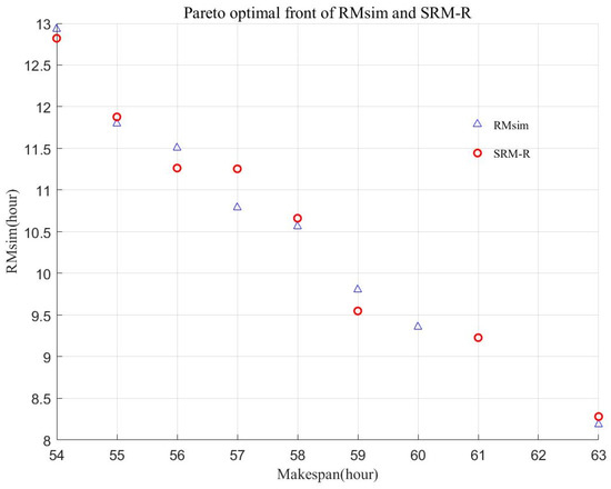
Figure 4.
The Pareto optimal front of the comparison robustness measures.
The variation range of RMsim is 8.18–12.93; (12.93–8.18)/12.93 = 31.9%. The range of Makespan is 54–64; (64–54)/64 = 15.6%, which means that the decision maker can choose any solution sacrificing at most 15.6% performance of the makespan while obtaining 31.9% improvements in the robustness. Comparing the Pareto optimal solutions obtained by SRM-R and RMsim in ten computational experiments, the set coverage value of the Pareto optimal fronts is 40% (RMsim dominates SRM-R, SC1) and 37.5% (SRM-R dominates RMsim, SC2), respectively. As for the Pareto front, the set coverage value is 50% (SC1) and 37.5% (SC2), respectively. The results denote that the SRM-R is effective to obtain robust schedule solutions with a significantly lower computational burden.
6. Conclusions
This paper addressed the RJSSP under stochastic deteriorating processing times, considering the resilience of production schedule, by formulating a surrogate model. To develop an effective SRM for robustness estimation, we provide a statistical approach that transforms the disturbances of stochastic deteriorating processing time to an estimated upper bound with a specified confidence level. Thereby, the formula of the disruption propagation is provided by analyzing the structure of the schedule. Additionally, then, we utilize the disruption propagation formula and the available processing time information to formulate the SRM-R. Moreover, we provide the MO-HEDA for solving the multi-objective RJSSP, in which the improved non-dominated sorting algorithm can increase computational efficiency by reducing the storage complexity and time complexity of the non-dominated sorting process.
Three groups of simulation experiments verified the effectiveness and the performance of the presented SRM-R. First, we investigated the correlation between the SRMs and the RMsim. The results demonstrated that the correlation of the presented SRM-R is higher than that of the existing SRMs, which indicates a better estimation accuracy of robustness. The second experiment compared the performance in obtaining the Pareto optimal solution obtained by using the presented SRM-R and the RMsim. According to the results, we concluded that the SRM-R can be used to estimate the robustness of RJSSP and obtain satisfying Pareto optimal solutions, with a tremendously lower computational burden. In addition, a case study further verified that the proposed surrogate model is effective for the studied RJSSP and production resilience can be effectively improved. Therefore, the presented SRM-R is a good choice for the decision makers, when computational efficiency is emphasized.
The limitation of the proposed SRM-R is the assumption that the processing time obeys the normal random separation. When the distribution type changes, the conditions for the disturbance propagation will change. Therefore, future research will further study the surrogate robustness measure under different probability distribution types, such as uniform distribution, lognormal distribution, and exponential distribution. Moreover, to further improve the production reliability, the surrogate measure of stability by using the disruption propagation formula should also be studied. Thereby, the multi-objective scheduling optimization approach for RJSSP will be provided, considering the makespan, the robustness, and the stability by using the presented surrogate measures. At the same time, this research may provide a theoretical basis for data-driven robust scheduling of job shops with the support of new technologies, such as digital twins and cloud manufacturing.
Author Contributions
Conceptualization, S.X. and Z.W.; methodology, S.X. and H.D.; software, S.X.; validation, S.X., Z.W. and H.D.; formal analysis, S.X.; investigation, S.X.; resources, Z.W.; data curation, Z.W.; writing—original draft preparation, S.X.; writing—review and editing, S.X., Z.W. and H.D.; visualization, S.X.; supervision, S.X. and H.D.; project administration, S.X.; funding acquisition, S.X. All authors have read and agreed to the published version of the manuscript.
Funding
This research was funded by Soft Science Key Project of Shanghai Science and Technology Innovation Action Plan (No. 20692193300]; the National Natural Science Foundation of China (No. U1904211); the Fundamental Research Funds for the Central Universities (No. 9160421005); Shanghai University Young Teacher Training Grant Program: (No. ZZSH20010).
Data Availability Statement
The authors confirm that the data supporting the findings of this study are available within the article.
Acknowledgments
The authors are thankful for the valuable comments and suggestions provided by the anonymous reviewers on the drafts of our paper. We are also grateful to the Shanghai Frontiers Science Center of “Full penetration” Far-Reaching Offshore Ocean Energy and Power.
Conflicts of Interest
The authors declare no conflict of interest.
References
- Abdel-Basset, M.; Mohamed, R.; Abouhawwash, M.; Chang, V.; Askar, S. A Local Search-Based Generalized Normal Distribution Algorithm for Permutation Flow Shop Scheduling. Appl. Sci. 2021, 11, 4837. [Google Scholar] [CrossRef]
- Liu, F.; Wang, S.; Hong, Y.; Yue, X. On the Robust and Stable Flowshop Scheduling Under Stochastic and Dynamic Disruptions. In IEEE Transactions on Engineering Management; IEEE: Manhattan, NY, USA, 2017; pp. 1–15. [Google Scholar]
- Zhang, R.; Wu, C. An Artificial Bee Colony Algorithm for the Job Shop Scheduling Problem with Random Processing Times. Entropy 2011, 13, 1708–1729. [Google Scholar] [CrossRef]
- Horng, S.-C.; Lin, S.-S.; Yang, F.-Y. Evolutionary algorithm for stochastic job shop scheduling with random processing time. Expert Syst. Appl. 2012, 39, 3603–3610. [Google Scholar] [CrossRef]
- Wang, S.; Wang, L.; Xu, Y.; Liu, M. An effective estimation of distribution algorithm for the flexible job-shop scheduling problem with fuzzy processing time. Int. J. Prod. Res. 2013, 51, 3778–3793. [Google Scholar] [CrossRef]
- Al-Hinai, N.; ElMekkawy, T.Y. Robust and stable flexible job shop scheduling with random machine breakdowns using a hybrid genetic algorithm. Int. J. Prod. Econ. 2011, 132, 279–291. [Google Scholar] [CrossRef]
- Xiong, J.; Xing, L.-N.; Chen, Y.-W. Robust scheduling for multi-objective flexible job-shop problems with random machine breakdowns. Int. J. Prod. Econ. 2013, 141, 112–126. [Google Scholar] [CrossRef]
- Xiong, H.; Shi, S.; Ren, D.; Hu, J. A survey of job shop scheduling problem: The types and models. Comput. Oper. Res. 2022, 142, 105731. [Google Scholar] [CrossRef]
- Aytug, H.; Lawley, M.A.; McKay, K.; Mohan, S.; Uzsoy, R. Executing production schedules in the face of uncertainties: A review and some future directions. Eur. J. Oper. Res. 2005, 161, 86–110. [Google Scholar] [CrossRef]
- Ouelhadj, D.; Petrovic, S. A survey of dynamic scheduling in manufacturing systems. J. Sched. 2009, 12, 417–431. [Google Scholar] [CrossRef]
- Sabuncuoglu, I.; Goren, S. Hedging production schedules against uncertainty in manufacturing environment with a review of robustness and stability research. Int. J. Comput. Integr. Manuf. 2009, 22, 138–157. [Google Scholar] [CrossRef]
- Sotskov, Y.N.; Werner, F. Sequencing and Scheduling with Inaccurate Data; Nova Science Publishers, Inc.: New York, NY, USA, 2014. [Google Scholar]
- Xiao, S.; Wu, Z.; Yu, S. A two-stage assignment strategy for the robust scheduling of dual-resource constrained stochastic job shop scheduling problems. IFAC-PapersOnLine 2019, 52, 421–426. [Google Scholar] [CrossRef]
- Palacios, J.J.; González-Rodríguez, I.; Vela, C.R.; Puente, J. Robust multiobjective optimisation for fuzzy job shop problems. Appl. Soft Comput. 2016, 56, 604–616. [Google Scholar] [CrossRef]
- Sotskov, Y.N.; Matsveichuk, N.M.; Hatsura, V.D. Two-Machine Job-Shop Scheduling Problem to Minimize the Makespan with Uncertain Job Durations. Algorithms 2019, 13, 4. [Google Scholar] [CrossRef]
- Zhang, J.; Yang, J.; Zhou, Y. Robust scheduling for multi-objective flexible job-shop problems with flexible workdays. Eng. Optim. 2016, 48, 1973–1989. [Google Scholar] [CrossRef]
- Herroelen, W.; Leus, R. Robust and reactive project scheduling: A review and classification of procedures. Int. J. Prod. Res. 2004, 42, 1599–1620. [Google Scholar] [CrossRef]
- Goren, S.; Sabuncuoglu, I. Optimization of schedule robustness and stability under random machine breakdowns and processing time variability. IIE Trans. 2009, 42, 203–220. [Google Scholar] [CrossRef]
- Gu, J.; Gu, M.; Cao, C.; Gu, X. A novel competitive co-evolutionary quantum genetic algorithm for stochastic job shop scheduling problem. Comput. Oper. Res. 2010, 37, 927–937. [Google Scholar] [CrossRef]
- Wu, S.D.; Byeon, E.-S.; Storer, R.H. A Graph-Theoretic Decomposition of the Job Shop Scheduling Problem to Achieve Scheduling Robustness. Oper. Res. 1999, 47, 113–124. [Google Scholar] [CrossRef]
- Xiao, S.; Sun, S.; Yang, H. Proactive Scheduling Research on Job Shop with Stochastically Controllable Processing Times. J. Northwest. Polytech. Univ. 2014, 6, 019. [Google Scholar]
- Xiao, S.; Sun, S.; Jin, J. Surrogate Measures for the Robust Scheduling of Stochastic Job Shop Scheduling Problems. Energies 2017, 10, 543. [Google Scholar] [CrossRef]
- Wu, Z.; Sun, S.; Xiao, S. Risk measure of job shop scheduling with random machine breakdowns. Comput. Oper. Res. 2018, 99, 1–12. [Google Scholar] [CrossRef]
- Wu, Z.; Yu, S.; Li, T. A Meta-Model-Based Multi-Objective Evolutionary Approach to Robust Job Shop Scheduling. Mathematics 2019, 7, 529. [Google Scholar] [CrossRef]
- Zahid, T.; Agha, M.H.; Schmidt, T. Investigation of surrogate measures of robustness for project scheduling problems. Comput. Ind. Eng. 2019, 129, 220–227. [Google Scholar] [CrossRef]
- Wu, Z.; Sun, S.; Yu, S. Optimizing makespan and stability risks in job shop scheduling. Comput. Oper. Res. 2020, 122, 104963. [Google Scholar] [CrossRef]
- Zheng, P.; Zhang, P.; Wang, J.; Zhang, J.; Yang, C.; Jin, Y. A data-driven robust optimization method for the assembly job-shop scheduling problem under uncertainty. Int. J. Comput. Integr. Manuf. 2020, 33, 1–16. [Google Scholar] [CrossRef]
- Yang, Y.; Huang, M.; Wang, Z.Y.; Zhu, Q.B. Robust scheduling based on extreme learning machine for bi-objective flexible job-shop problems with machine breakdowns. Expert Syst. Appl. 2020, 158, 113545. [Google Scholar] [CrossRef]
- Dui, H.; Xu, Z.; Chen, L.; Xing, L.; Liu, B. Data-Driven Maintenance Priority and Resilience Evaluation of Performance Loss in a Main Coolant System. Mathematics 2022, 10, 563. [Google Scholar] [CrossRef]
- Mao, X.; Lou, X.; Yuan, C.; Zhou, J. Resilience-Based Restoration Model for Supply Chain Networks. Mathematics 2020, 8, 163. [Google Scholar] [CrossRef]
- Qi, Q.; Meng, Y.; Zhao, X.; Liu, J. Resilience Assessment of an Urban Metro Complex Network: A Case Study of the Zhengzhou Metro. Sustainability 2022, 14, 11555. [Google Scholar] [CrossRef]
- Xiao, S.; Wu, Z.; Sun, S.; Jin, M. Research on the Dual-resource Constrained Robust Job Shop Scheduling Problems. J. Mech. Eng. 2021, 57, 227–239. [Google Scholar]
- Wang, K.; Choi, S.H.; Lu, H. A hybrid estimation of distribution algorithm for simulation-based scheduling in a stochastic permutation flowshop. Comput. Ind. Eng. 2015, 90, 186–196. [Google Scholar] [CrossRef]
- Graham, R.L.; Lawler, E.L.; Lenstra, J.K.; Kan, A.R. Optimization and approximation in deterministic sequencing and scheduling: A survey. Ann. Discret. Math. 1979, 5, 287–326. [Google Scholar]
- Leon, V.J.; Wu, S.D.; Storer, R.H. Robustness measures and robust scheduling for job shops. IIE Trans. 1994, 26, 32–43. [Google Scholar] [CrossRef]
- Hazır, Ö.; Haouari, M.; Erel, E. Robust scheduling and robustness measures for the discrete time/cost trade-off problem. Eur. J. Oper. Res. 2010, 207, 633–643. [Google Scholar] [CrossRef]
- Goren, S.; Sabuncuoglu, I.; Koc, U. Optimization of schedule stability and efficiency under processing time variability and random machine breakdowns in a job shop environment. Nav. Res. Logist. 2012, 59, 26–38. [Google Scholar] [CrossRef]
- Larranaga, P.; Lozano, J.A. Estimation of Distribution Algorithms: A New Tool for Evolutionary Computation; Springer: New York, NY, USA, 2002. [Google Scholar]
- Xiao, S.; Sun, S.; Guo, H.; Jin, M.; Yang, H. Hybrid Estimation of Distribution Algorithm for Solving the Stochastic Job Shop Scheduling Problem. J. Mech. Eng. 2015, 51, 27–35. [Google Scholar] [CrossRef]
- Deb, K.; Pratap, A.; Agarwal, S.; Meyarivan, T. A Fast and Elitist Multiobjective Genetic Algorithm: NSGA-II. In IEEE Transactions on Evolutionary Computation; IEEE: Manhattan, NY, USA, 2002; Volume 6, p. 15. [Google Scholar]
- Valledor, P.; Gomez, A.; Puente, J.; Fernandez, I. Solving Rescheduling Problems in Dynamic Permutation Flow Shop Environments with Multiple Objectives Using the Hybrid Dynamic Non-Dominated Sorting Genetic II Algorithm. Mathematics 2022, 10, 2395. [Google Scholar] [CrossRef]
- Muth, J.F.; Thompson, G.L. Industrial Scheduling; Prentice-Hall: Hoboken, NJ, USA, 1963. [Google Scholar]
- Lawrence, S. Resource constrained project scheduling: An experimental investigation of heuristic scheduling techniques (Supplement); Carnegie-Mellon University: Pennsylvania, PA, USA, 1984. [Google Scholar]
- Ahmadi, E.; Zandieh, M.; Farrokh, M.; Emami, S.M. A multi objective optimization approach for flexible job shop scheduling problem under random machine breakdown by evolutionary algorithms. Comput. Oper. Res. 2016, 73, 56–66. [Google Scholar] [CrossRef]


Publisher’s Note: MDPI stays neutral with regard to jurisdictional claims in published maps and institutional affiliations. |
© 2022 by the authors. Licensee MDPI, Basel, Switzerland. This article is an open access article distributed under the terms and conditions of the Creative Commons Attribution (CC BY) license (https://creativecommons.org/licenses/by/4.0/).