Abstract
As an important data analysis method in the field of machine learning and data mining, feature learning has a wide range of applications in various industries. The traditional multidimensional scaling (MDS) maintains the topology of data points in the low-dimensional embeddings obtained during feature learning, but ignores the discriminative nature between classes of low-dimensional embedded data. Thus, the discriminative multidimensional scaling based on pairwise constraints for feature learning (pcDMDS) model is proposed in this paper. The model enhances the discriminativeness from two aspects. The first aspect is to increase the compactness of the new data representation in the same cluster through fuzzy k-means. The second aspect is to obtain more extended pairwise constraint information between samples. In the whole feature learning process, the model considers both the topology of samples in the original space and the cluster structure in the new space. It also incorporates the extended pairwise constraint information in the samples, which further improves the model’s ability to obtain discriminative features. Finally, the experimental results on twelve datasets show that pcDMDS performs and higher than PMDS model in terms of accuracy and purity.
Keywords:
discriminative feature learning; multidimensional scaling; fuzzy k-means; pairwise constraint propagation; iterative majorization algorithm MSC:
62P25
1. Introduction
The high-dimensional nature of large amounts of image data, text data, and video data is inevitable in today’s big data era. Although image data and text data are simple and intuitive for humans, for machine learning models, there is a dimensional disaster. Because the direct use of raw data will not only increase the processing time of subsequent machine learning models, but may also reduce the performance of classification models and clustering models due to the influence of information such as redundancy and noise in the data. Based on this, how to obtain a more discriminative feature from the raw data has also become a research objective for many scholars.
In feature learning, supervised, semi-supervised and unsupervised feature learning methods are classified by whether or not the annotation information of the data is used in the learning process. The classical methods for unsupervised feature learning, semi-supervised feature learning and unsupervised feature learning are principal component analysis (PCA) [1], semi-supervised dimensionality deduction (SSDR) [2] and linear discriminant analysis (LDA) [3], respectively. PCA, SSDR and LDA are all linear feature learning methods, which have the advantage of fast computation and the ability to quickly compute the data representation of a new sample through the projection matrix when a new sample arrives. In contrast, nonlinear feature learning based on stream learning allows the low-dimensional data representation to preserve the local topology of the original data as much as possible, such as locally linear embedding (LLE) [4], multidimensional scaling (MDS) [5] and laplacian eigenmaps (LE) [6], etc. Nonlinear feature learning can discover the potential flow structure inside the data well, but face the problem of new samples [7], so there are also a number of algorithms that maintain the local topology as much as possible in the projection process. For example, locality preserving projection (LPP) [8] and neighborhood preserving embedding [9] are projection matrices added to LE and LLE, respectively.
Feature learning has important research significance because of its many applications, such as data visualization [10], information retrieval [11], and clustering [12]. The MDS, as a commonly used streaming learning method, considers the distance information between samples in the feature learning process, but ignores the discriminative nature between data categories. Based on this, a discriminative multidimensional scaling based on pairwise constraints for feature learning (pcDMDS) is proposed in this paper in order to obtain more discriminative features.
The main contributions of this paper are shown below.
- A feature learning algorithm named pcDMDS is proposed, and its corresponding target formula is designed. The target formula reflects the topological and discriminative nature of learning, and the cluster structure is discovered while learning the low-dimensional data representation. It makes the low-dimensional data representation of the same cluster closer.
- The objective function is approximated using an iterative optimization method, and the corresponding algorithm is designed according to the inference process.
- Comparative experiments are conducted using public datasets and evaluation criteria, and the results show that the low-dimensional embeddings obtained by the algorithm are more discriminative.
The remainder of this paper is organized as follows. In Section 2, existing works that related to this paper is reviewed. In Section 3, some preliminaries about our work are introduced. In Section 4, the details of the proposed model, including objective function and inference are illustrated. Experiments and results are described in Section 5. Finally, conclusions are drawn in Section 6.
2. Related Work
As a feature learning method that maintains the non-similarity of samples (generally distance), the MDS is widely used because of its simplicity and efficiency. Feature learning based on MDS can be divided into two categories [13], one is metric multidimensional scaling (MMDS) and the other one is non-metric multidimensional scaling (NMDS). In MMDS, the learned low-dimensional data representation is to preserve the distance of the original data as much as possible. But in NMDS, the low-dimensional data representation is to maintain the relationship of distance of the original data. Since the model proposed in this paper is a MDS of metrics, the MDS of metrics is described in detail below, and MDS generally refers to MMDS.
Different MDS methods have been proposed successively. The most classical MDS is to give the distance between samples and then find a suitable low-dimensional embedding. This method belongs to a nonlinear feature learning method, so that the sample distance between the low-dimensional embedding points keeps the distance corresponding to the original sample as much as possible, and its disadvantage is that it faces the problem of new samples. Webb [14] introduced a set of basis functions for feature mapping, and then achieved dimensionality reduction through a projection matrix. At the same time, the new data representation keeps the Euclidean distance of the original samples as much as possible, and an iterative update method was proposed to optimize the projection matrix. As an important manifold learning method, isometric feature mapping [15] uses the geodesic distance between samples to represent the dissimilarity between samples, and finally uses classical MDS to get low-dimensional embedding of data. Bronstein et al. [16] proposed a generalized multidimensional scaling (GMDS), which uses a non-euclidean distance to represent the non-similarity of samples, and applied GMDS to 3D face matching. In order to enhance the discriminativeness of the features learned by MDS, Biswas [17] not only considered that the low-dimensional embedding points should keep the distance between the original images, but also considered that the distance between the low-dimensional embedding points corresponding to the same face should be as small as possible.
Clustering, as an unsupervised machine learning method, is widely used in many fields [18,19,20], and its purpose is to divide data into different clusters or subsets by some criteria. In order to efficiently discover potential cluster structures in data, different scholars have proposed different clustering algorithms, such as k-means (KM) algorithm [21], affinity propagation (AP) algorithm [22], and density peak (DP) algorithm [23]. With the proposal and refinement of fuzzy set theory, fuzzy clustering was proposed [24]. Unlike hard clustering such as k-means, soft clustering algorithms such as fuzzy clustering can not only discover the cluster structure among data efficiently, but also give the degree of affiliation between samples and class clusters, which can discover the overlapping class cluster structure well.
Fuzzy k-means was proposed by Bezdek et al. [24], which adopted the idea of fuzzy sets. They believe that there is a degree of attribution between a sample and a cluster ranging from 0 to 1. To improve the clustering performance of fuzzy k-means, Wang et al. [25] proposed a fuzzy k-means model based on the Euclidean distance with weights by considering the feature weights while calculating the distance. The traditional FKM fails when the input sample point information is not known and only the non-similarity information of sample points is available. Therefore, Hathaway et al. [26] proposed a non-euclidean relational fuzzy clustering, which can complete the fuzzy clustering under the condition of only given the dissimilarity between sample points. In order to adopt the clustering algorithm to noisy data, Nie et al. [27] combined fuzzy k-means with principal component analysis so that fuzzy k-means can be performed in the low-dimensional subspace obtained by principal component analysis. To obtain the potential cluster structure of the data on multi-view data, Zhu et al. [28] proposed an adaptive weighted multi-view clustering method. This method can not only automatically discover the importance, dispersion and other information of each view from multi-view data, but also synthesize the common information of each view to accomplish the clustering task.
Paired constraint information is widely used in feature learning to enhance the discriminant of the learned features because of its ability to provide similar relationships between samples. Zhang et al. [2] proposed a semi-supervised dimensionality reduction method based on paired constraint information, whose idea is to obtain new sample points by transforming the matrix so that the points with must-connect constraints are close together after the transformation, while the points with do-not-connect constraints are far away after the transformation. Du et al. [29] applied constraint transferring to dimensionality reduction and proposed a new semi-supervised feature learning method. The method first requires a pairwise constraint matrix with only 1, 0 and −1 values initially, where 1 means constraints must be connected, −1 means constraints do not connected and 0 means the constraint information is unknown. Then the constraint transferring algorithm is used to extend the constraint information to other samples. Then it constructs a new weight matrix using the extended constraint matrix, and finally uses the LPP algorithm for the new data representation.
3. Preliminaries
3.1. Multidimensional Scaling
The classical MDS is a nonlinear feature learning method. Its characteristic is that when only the dissimilarity between any two points is given, the corresponding new data representation can be directly obtained so that the Euclidean distance between samples is as equal to the given dissimilarity as possible, but it faces the problem of new samples. Webb [14] proposed the projective MDS (PMDS), so that the new data representation can be obtained from the original data representation by projection transformation. In this paper, a PMDS-based feature learning method is proposed and its principles are described in detail below.
Given the original data matrix , where n and N denote the dimensionality and the number of the original samples, respectively. The learned low-dimensional data representation , where l denotes the dimensionality of the low-dimensional data representation. The loss function of MDS, a feature learning method that maintains the sample distance, is [30]:
denotes the distance between the original data points and , and denotes the distance between the corresponding low-dimensional data representation and . And is a non-negative symmetric weight matrix, with larger indicating a greater desire for to be close to , and the literature [6] gives two ways of constructing the weights.
- Heat kernel weighting: if is a near neighbor to or is a near neighbor to , otherwise , where t is a real number.
- 0–1 weights: if is a near neighbor to or is a near neighbor to , otherwise .
The MDS in Equation (1) is a nonlinear feature learning method that obtains a direct low-dimensional data representation Y. If new data arrives, its corresponding low-dimensional data representation cannot be obtained directly, that is, the so-called new sample problem. Webb incorporated the projection matrix into the MDS by means of pre-given radial basis functions to achieve nonlinear transformations, and proposed the PMDS, whose objective formulation is [14]:
denotes the two-parametric number of vectors and denotes the projection matrix, and it can be seen that Y is directly projected from X.
3.2. Fuzzy k-Means Clustering
Fuzzy clustering can give the degree of affiliation of samples with clusters, and the objective formula for fuzzy k-means is:
is the affiliation matrix, denotes the affiliation of with cluster , and denotes the fuzzy index weights.
3.3. Pairwise Constraint Transmission
Given a sample , and the pairwise constraint matrix . if there is a must-connect constraint between samples and , if there is a do-not-connect constraint between samples and , and , if the constraint between and is unknown.
The constraint-passing algorithm is to extend the constraint matrix P to obtain more pairwise constraint information. The result matrix is , and F has the following properties:
- takes the value in the range of [−1, 1], and the larger the absolute value, the higher the confidence of the constraint information.
- means that the constraint between and is must-connect.
- means that the constraint between and is do-not-connect.
- means that the constraint information is unknown.
4. Proposed Method
4.1. Discriminative Multidimensional Scaling Based on Pairwise Constraints for Feature Learning
The overall process of model pcDMDS is shown in Figure 1, which shows that after obtaining some of the pairwise constraint information through data X, more constraint information is first extended by the constraint transferring algorithm. For the extended constraint information, its value is [−1, 1]. If the value is greater than 0, it indicates a must-connect constraint, while if it is less than 0, it indicates a do-not-connect constraint. And the larger the absolute value, the higher the confidence level of the constraint. After obtaining the extended pairwise constraint information, for each iteration of the model, we hope to maintain the topology of the samples on the one hand. On the other hand, we hope to find the cluster structure within the samples and make the data representations of the samples in the same cluster close to their cluster centers. Furthermore, we hope to make the data representations of the samples with the must-connect constraints close to each other and the data representations of the samples with the do-not-connect constraints far from each other through pairwise constraints. After several iterations, the model can reach a balance between these three aspects. Thus, it further improves the discriminative properties of the learned features. After the model converges or reaches the maximum number of iterations, the new data representation is obtained by transforming the matrix.
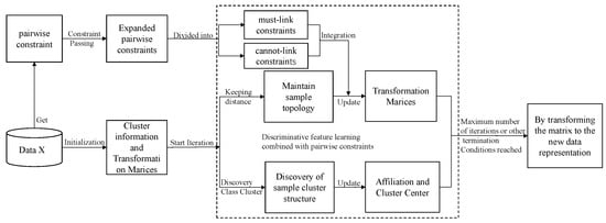
Figure 1.
The overall process of discriminative multidimensional scalar learning based on pairwise constraints.
Following this idea, the loss function can be described as the minimum of . Moreover,
In Equation (4), ML denotes the set of the indexes of the sample pairs with must-connect constraints and denotes the set of the indexes of the sample pairs with do-not-connect constraints. denotes the number of sample pairs with must-connect constraints, and is the size of the set. Similarly, denotes the number of sample pairs with do-not-connect constraints, and is the size of the set. denotes the confidence of the pairwise constraint between samples and , which takes the values [0, 1], and a larger value indicates a higher confidence of the pairwise constraint and a symmetric matrix.
From Equation (4), it can be seen that the objective formulation of the pcDMDS model can be divided into three parts. It can be seen that the pcDMDS model is a balance among these three terms.
- i.
- The first part is used to make the Euclidean distance between any samples and the new data representation corresponding to keeps the Euclidean distance in the original space as much as possible, which reflects the feature learning process in which the new data representation keeps the topology in the original data representation.
- ii.
- The second part is used to automatically discover the cluster structure in the samples and make the data representation in the same cluster close to its cluster center in the new data representation, increasing the compactness of the new data representation in the same cluster, and reflecting the unsupervised way to enhance the discriminative nature of the learned data representation and adjust its weight by the parameter .
- iii.
- The third term is the loss term of the pairwise constraint, which aims to make the data representation of sample points with the must-connect constraint close and the data representation of sample points with the do-not-connect constraint. The third term is the pairwise constraint loss term, which aims to make the data representations of sample points with the must-connect constraint close and those of sample points with the do-not-connect constraint far away, thus further enhancing the model’s ability to learn discriminative features and controlling its weights by the parameter .
To simplify Equation (4) for subsequent optimization, note the matrix , whose elements are defined as:
Since , it follows that . Then Equation (4) can be rewritten as:
4.2. The Inference of Discriminative Multidimensional Scaling Based on Pairwise Constraints for Feature Learning
For the objective Equation (6), the parameters to be solved are the transformation matrix W, the samples and cluster affiliation matrix U, and the cluster center matrix V. Since the closed-form solutions of Equation (6) with respect to W, U, and V cannot be obtained directly, an iterative optimization approach is used for solving the problem.
(1) Fix U and and update W. At this point the target equation in Equation (6) is a function of W only and can be expressed as:
to facilitate the solution, first rewrite :
Since , denotes the trace of the matrix, a simplification of the second term in Equation (7) gives:
, and are all diagonal arrays,
The objective function in Equation (8) can be optimized using the IMA [5,14,17] algorithm, the constructed auxiliary function is , which is defined as:
The definition of in Equation (11) is:
In Equation (13), .
Calculate the gradient of W with respect to Equation (11) and set the gradient to be 0, then we have the update equation of W:
(2) Fix the matrices W and V, and solve for U. At this point, the first and third terms in Equation (6) are constant terms, and the optimization of Equation (6) is equivalent to the optimization of:
Using the Lagrangian multiplier method [31]:
By:
solve the update equation for as:
The iterative update of the U matrix is given by:
, denotes the set of positive integers less than or equal to C, and denotes the number of elements in the set . It means that when there exists a sample point that happens to be the cluster center of multiple clusters, has equal affiliation with these clusters, both being .
(3) Fix W and U, and update V. Similar to step (2):
Calculate the partial derivative with respect to for Equation (20):
4.3. Algorithm
4.3.1. Algorithm Description
It can be seen from Algorithm 1 that the algorithm flow of pcDMDS is mainly divided into two processes. The first process is mainly to expand pairwise constraint information through constraint transferring. The second process is to update it iteratively according to the update formulas of W, U and V, and output the transformation matrix after the iteration is completed. Specifically, for the first process, the pairwise constraint matrix P is first constructed according to the set of sample pairwise constraints. Then the extended pairwise constraint information F is obtained through the constraint transfer algorithm, and F is post-processed and assigned to . Then the distance matrices D, S and A are calculated respectively, and then the W, V and U matrices are initialized. The second process starts the iteration process, updating W, U and V in turn, and stops iteration when W and U are stable or reach the maximum number of iterations. Finally, the transformation matrix W is returned.
| Algorithm 1: pcDMDS feature learning algorithm |
 |
4.3.2. Study on Computational Complexity
The time complexity of the model is discussed. According to the algorithm flow in Algorithm 1, pcDMDS needs to call the constraint passing algorithm of the with a time complexity of . The time complexity of the matrix is . The symmetric matrix of size and its Moore-Penrose inverse can be obtained by singular value decomposition, and since the time complexity of singular value decomposition is [32], the time complexity of updating W once is according to Equation (14). According to Equation (19), the time complexity of updating the matrix U once is . From Equation (22), it is known that the time complexity of updating the cluster center matrix V once is . Considering that the updates of matrices W, U and V are performed sequentially, and the time complexity of the three updates and the time complexity of constraint passing are combined, it is known that the time complexity of the pcDMDS algorithm is , where T is the maximum number of iterations.
Then, the space complexity of the model is discussed. The input data matrix X has size of . The space complexity of P, F, D and S are . The space complexity of A is . W, V and U has the size of , and , respectively. During the iteration, the space complexity of and are and . The space complexity of is . The space complexity of W is . The space complexity of Y is . Therefore, the total space complexity is .
4.3.3. Visualization
Figure 2 shows the visualization results of the wine dataset with 178 samples, 3 categories, and the number of attributes of each sample is 13. It can be seen from the visualization results in Figure 2a that the boundaries of different categories in the 2D data representation are fuzzy and unclear, that is, the discriminability between different categories has not been improved, and since the MDS method maintains the distance between samples, the samples in the same category are not more compact. In order to more intuitively show that pcDMDS can learn more discriminative features, the visualization result graph of pcDMDS is shown in Figure 2b. By comparing Figure 2a,b, it can be found that compared with MDS, pcDMDS has a more compact sample distribution in the same category in the new data representation, and the boundaries between different categories are clearer, which makes the learning features more discriminative.
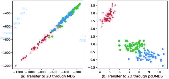
Figure 2.
Visualization of wine dataset after dimensionality reduction using MDS and pcDMDS.
5. Experiments
5.1. Datasets
The datasets used for the experiments on the discriminative multidimensional scalar feature learning algorithm based on pairwise constraints are from 12 publicly available datasets in the MSRA-MM [33] database. Table 1 describes the details of the 12 datasets used.

Table 1.
Datasets.
5.2. Experimental Setting
The pairwise constraint loss terms in pcDMDS are controlled by the parameter to control their weights. The pairwise constraint information in the experiment is obtained directly from the ten percent label information, and then the constraint transferring algorithm obtains the extended constraint information as the final pairwise constraint information. For the pcDMDS algorithm, the parameter is set to , and the parameter in the constraint transferring algorithm is set to . In order to reduce the differences in the experimental results, all feature learning algorithms are run 10 times in the experiments, and then the average of the 10 times is taken as the final result.
The experiments of pcDMDS algorithm are to evaluate the ability of pcDMDS to learn discriminative features. The experiments are designed in such a way that multiple clustering experiments are performed on the low-dimensional data representation obtained from the original data, the low-dimensional data representation obtained from the PMDS algorithm and the data representation obtained from pcDMDS, respectively. If the data representation is more discriminative, the clustering algorithm performs better. The selected clustering algorithms include KM, AP and DP.
5.3. Evaluation Metric
Since features with discriminative properties tend to improve the performance of subsequent machine learning tasks, the discriminative properties of the learned features can be evaluated by evaluating the performance of subsequent machine learning tasks. The subsequent machine learning tasks include clustering tasks and classification tasks, so the performance of the learned features is evaluated by using the evaluation metrics of clustering and classification.
5.3.1. Accuracy
Accuracy, a common metric for clustering, measures the degree of difference between the sample cluster results given by a clustering model and the true labels of the samples. The calculation of clustering accuracy and classification accuracy is slightly different. For clustering, the accuracy is computed as [34].
N denotes the number of sample points, and is a function that maps the cluster index to the category label. and denote the category label and the cluster index of sample point , respectively. is a function whose value is 1 when . Otherwise, it is 0. For the classification task, denotes the classifier’s predicted category label, at this time can be considered as a constant mapping. The output value is equal to the input value.
5.3.2. Purity
Purity is a common metric used to measure the performance of clustering algorithms and is defined as [35]:
N denotes the number of sample points, C denotes the number of clusters, k denotes the cluster index, and q is the number of classes. In general, q is equal to C. denotes the number of samples with class label r in the k cluster.
5.3.3. Friedman Test
Friedman statistic is a statistical method for non-parametric testing to evaluate the overall difference in performance of a set of algorithms on different datasets. Friedman statistic requires first getting the ranking of each algorithm’s performance on the same dataset, with the best performing algorithm ranked as 1, the next best algorithm ranked as 2, and so on to get the rankings of all algorithms, and if there is the same performance, the average ranking value is taken. The ranking value of an algorithm is also called rank value. Specifically, the Friedman statistic is defined as [36]:
The a denotes the number of datasets, b denotes the number of algorithms, , denotes the rank value of the j-th algorithm on the i-th dataset, and it can be seen that denotes the average rank value of the j-th algorithm on all datasets, obeys the chi-square distribution with degrees of freedom .
Iman and Davenport improved the deficiencies of the Friedman statistic by proposing a better statistic defined as [37]:
is the F distribution with degrees of freedom and . The p-value is obtained by looking up the table, and the significance of the differences between all algorithms is evaluated based on the p-value.
5.4. Results
Table 2 and Table 3 give the accuracy and purity results obtained by clustering the 12 data sets by KM, AP and DP under three different data representations, respectively. Specifically, in Table 2, columns KM, AP and DP are the clustering accuracies of the three algorithms on the original data representation. PMDS-KM, PMDS-AP and PMDS-DP are the clustering accuracies of the three clustering algorithms on the low-dimensional data representation obtained by the PMDS algorithm. pcDMDS-KM, pcDMDS-AP and pcDMDS-DP are the clustering accuracies of the three clustering algorithms on the low-dimensional data representation obtained by the pcDMDS algorithm. The Avg column is the mean of columns KM, AP and DP. Column PMDS-Avg is the mean value of columns PMDS-KM, PMDS-AP and PMDS-DP. Similarly, column pcDMDS-Avg is the mean value of columns pcDMDS-KM, pcDMDS-AP and pcDMDS-DP. The meaning of the table headers in Table 3 is similar to that in Table 2, except that the data in the table are purity rather than accuracy, which is not repeated here.
Table 2.
Accuracy of clustering with different data representations.
Table 3.
Purity of clustering with different data representations.
From Table 2, it can be seen that 10 of the models with the highest accuracy in these 12 datasets are on the data representation learned by pcDMDS features (bolded data in the table), and 2 are on the original data representation, which indicates that pcDMDS can improve the discriminatory performance of the data representation. Moreover, for the same clustering algorithm, the performance exhibited on the data representation obtained by the pcDMDS algorithm is overwhelmingly better than the original data representation and the PMDS data representation. In addition, in terms of the average accuracy, the 12 highest average accuracies are in the feature representation of the pcDMDS algorithm, and the average accuracy of the data representation obtained by the pcDMDS algorithm is and higher than that of the PMDS and the original space, respectively. This also reflects that the data representation obtained after the DMDS feature learning algorithm can improve the performance of the subsequent machine learning compared with the PMDS and the original data representation.
The overall performance of the model is then evaluated based on the Friedman statistic. Based on the last three columns of Table 2, the ranking values for the performance of different data representations in each dataset can be first derived. The average ranking values of 2.4583, 2.5416 and 1 for Avg, PMDS-Avg and pcDMDS-Avg on the 12 datasets can be calculated, respectively. Since there are 12 datasets with three types of averages, obeys a degree of freedom of and for the F distribution. From the distribution, the p-value can be calculated as , so the original hypothesis is rejected at a high significance level, and the comprehensive evaluation of the pcDMDS algorithm outperforms the PMDS algorithm. The data representation obtained by the pcDMDS algorithm is more discriminative than the data representation obtained by PMDS and the original data representation.
Table 3 lists the purity of the clustering results on the different data representations. It can be seen that the 12 highest purity are on the data representation of pcDMDS. Overall, the clustering performance on pcDMDS is better than PMDS and raw space. Also, the average purity of the data representation obtained by the pcDMDS algorithm is and higher than that of the PMDS and the original space, respectively.
Similarly, the Friedman statistic is used to evaluate the overall performance of the model. According to the last three columns of Table 3, the average ranking values of Avg, PMDS-Avg and pcDMDS-Avg can be obtained as 2.5, 2.5 and 1, respectively. The Friedman statistic can be calculated as , and then the Iman-Davenport as . The p-value can be calculated from the distribution as , so the original hypothesis is rejected at a higher significance level, and the combined evaluation of pcDMDS algorithm is better than PMDS and the original space.
In terms of accuracy and purity, it can be seen that the data representation obtained by pcDMDS has a better performance for subsequent clustering algorithms than the original data representation and the data representation obtained by PMDS, which can learn more discriminative features. For big datasets, pcDMDS can enhance the discriminativeness by considering both the topology of samples in the original space and the cluster structure in the new space, and also incorporating the extended pairwise constraint information in the samples.
6. Conclusions
In this paper, a feature learning algorithm named pcDMDS is proposed and the discriminability is enhanced in two aspects. Firstly, the ability to automatically discover clusters in samples by fuzzy k-means, so that new data representations corresponding to samples in the same cluster are close to the cluster center during feature learning. Then the pairwise constraint information between more samples, noted as extended pairwise constraint information, is obtained by a constraint transferring algorithm based on the pairwise constraint information between a given part of samples. In the whole process of feature learning, the ability of the original model to obtain discriminative features is further improved. Because pcDMDS not only considers the topological structure of the sample in the original space and the cluster structure in the new space, but also incorporates the extended pairwise constraint information in the sample. However, the effect of different values of parameter on the clustering performance of pcDMDS was analyzed in pcDMDS, but the values are fixed, so the effect of and can be considered jointly in the future. Plus, the model does not use incremental learning, and it can be put into research in the future work.
Author Contributions
Conceptualization, L.Z., B.P., H.T. and H.W.; methodology, L.Z., B.P. and H.T.; software, L.Z., B.P., H.T. and H.W.; validation, C.L., Z.L. and H.T.; formal analysis, L.Z.; investigation, Z.L.; resources, B.P., H.T., H.W. and C.L.; data curation, L.Z.; writing—original draft, L.Z., B.P., H.T., H.W. and C.L.; writing—review and editing, L.Z., B.P., H.T., H.W., C.L. and Z.L.; visualization, L.Z., B.P. and H.W.; supervision, H.W. and C.L.; project administration, Z.L. All authors have read and agreed to the published version of the manuscript.
Funding
This research work was supported by the Science and Technology Project of State Grid Sichuan Electric Power Company (52199722000Y).
Data Availability Statement
Data are freely available from MSRA.
Conflicts of Interest
The authors declare no conflict of interest.
Correction Statement
This article has been republished with a minor correction to the Funding statement. This change does not affect the scientific content of the article.
References
- Wold, S.; Esbensen, K.; Geladi, P. Principal component analysis. Chemom. Intell. Lab. Syst. 1987, 2, 37–52. [Google Scholar] [CrossRef]
- Zhang, D.; Zhou, Z.H.; Chen, S. Semi-supervised dimensionality reduction. In Proceedings of the 2007 SIAM International Conference on Data Mining, Minneapolis, MI, USA, 26–28 April 2007; SIAM: Philadelphia, PA, USA, 2007; pp. 629–634. [Google Scholar]
- Martinez, A.M.; Kak, A.C. Pca versus lda. IEEE Trans. Pattern Anal. Mach. Intell. 2001, 23, 228–233. [Google Scholar] [CrossRef]
- Roweis, S.T.; Saul, L.K. Nonlinear dimensionality reduction by locally linear embedding. Science 2000, 290, 2323–2326. [Google Scholar] [CrossRef] [PubMed]
- Borg, I.; Groenen, P.J. Modern Multidimensional Scaling: Theory and Applications; Springer Science & Business Media: Berlin/Heidelberg, Germany, 2005. [Google Scholar]
- Belkin, M.; Niyogi, P. Laplacian eigenmaps for dimensionality reduction and data representation. Neural Comput. 2003, 15, 1373–1396. [Google Scholar] [CrossRef]
- Bengio, Y.; Paiement, J.F.; Vincent, P.; Delalleau, O.; Roux, N.; Ouimet, M. Out-of-sample extensions for lle, isomap, mds, eigenmaps, and spectral clustering. Adv. Neural Inf. Process. Syst. 2003, 16, 177–184. [Google Scholar]
- He, X.; Niyogi, P. Locality preserving projections. Adv. Neural Inf. Process. Syst. 2003, 16, 153–160. [Google Scholar]
- He, X.; Cai, D.; Yan, S.; Zhang, H.J. Neighborhood preserving embedding. In Proceedings of the Tenth IEEE International Conference on Computer Vision (ICCV’05), Volume 1, Beijing, China, 17–21 October 2005; IEEE: Piscataway, NJ, USA, 2005; Volume 2, pp. 1208–1213. [Google Scholar]
- Tsai, F.S. Dimensionality reduction techniques for blog visualization. Expert Syst. Appl. 2011, 38, 2766–2773. [Google Scholar] [CrossRef]
- Ingram, S.; Munzner, T. Dimensionality reduction for documents with nearest neighbor queries. Neurocomputing 2015, 150, 557–569. [Google Scholar] [CrossRef]
- Xu, J.; Han, J.; Nie, F. Discriminatively embedded k-means for multi-view clustering. In Proceedings of the IEEE Conference on Computer Vision and Pattern Recognition, Las Vegas, NV, USA, 27–30 June 2016; pp. 5356–5364. [Google Scholar]
- Saeed, N.; Nam, H.; Haq, M.I.U.; Muhammad Saqib, D.B. A survey on multidimensional scaling. ACM Comput. Surv. (CSUR) 2018, 51, 1–25. [Google Scholar] [CrossRef]
- Webb, A.R. Multidimensional scaling by iterative majorization using radial basis functions. Pattern Recognit. 1995, 28, 753–759. [Google Scholar] [CrossRef]
- Tenenbaum, J.B.; Silva, V.d.; Langford, J.C. A global geometric framework for nonlinear dimensionality reduction. Science 2000, 290, 2319–2323. [Google Scholar] [CrossRef] [PubMed]
- Bronstein, A.M.; Bronstein, M.M.; Kimmel, R. Generalized multidimensional scaling: A framework for isometry-invariant partial surface matching. Proc. Natl. Acad. Sci. USA 2006, 103, 1168–1172. [Google Scholar] [CrossRef] [PubMed]
- Biswas, S.; Bowyer, K.W.; Flynn, P.J. Multidimensional scaling for matching low-resolution face images. IEEE Trans. Pattern Anal. Mach. Intell. 2011, 34, 2019–2030. [Google Scholar] [CrossRef] [PubMed]
- Janani, R.; Vijayarani, S. Text document clustering using spectral clustering algorithm with particle swarm optimization. Expert Syst. Appl. 2019, 134, 192–200. [Google Scholar] [CrossRef]
- McDowell, I.C.; Manandhar, D.; Vockley, C.M.; Schmid, A.K.; Reddy, T.E.; Engelhardt, B.E. Clustering gene expression time series data using an infinite Gaussian process mixture model. PLoS Comput. Biol. 2018, 14, e1005896. [Google Scholar] [CrossRef]
- Alashwal, H.; El Halaby, M.; Crouse, J.J.; Abdalla, A.; Moustafa, A.A. The application of unsupervised clustering methods to Alzheimer’s disease. Front. Comput. Neurosci. 2019, 13, 31. [Google Scholar] [CrossRef]
- Likas, A.; Vlassis, N.; Verbeek, J.J. The global k-means clustering algorithm. Pattern Recognit. 2003, 36, 451–461. [Google Scholar] [CrossRef]
- Frey, B.J.; Dueck, D. Clustering by passing messages between data points. Science 2007, 315, 972–976. [Google Scholar] [CrossRef]
- Rodriguez, A.; Laio, A. Clustering by fast search and find of density peaks. Science 2014, 344, 1492–1496. [Google Scholar] [CrossRef]
- Bezdek, J.C.; Ehrlich, R.; Full, W. FCM: The fuzzy c-means clustering algorithm. Comput. Geosci. 1984, 10, 191–203. [Google Scholar] [CrossRef]
- Wang, X.; Wang, Y.; Wang, L. Improving fuzzy c-means clustering based on feature-weight learning. Pattern Recognit. Lett. 2004, 25, 1123–1132. [Google Scholar] [CrossRef]
- Hathaway, R.J.; Bezdek, J.C. NERF c-means: Non-Euclidean relational fuzzy clustering. Pattern Recognit. 1994, 27, 429–437. [Google Scholar] [CrossRef]
- Nie, F.; Zhao, X.; Wang, R.; Li, X.; Li, Z. Fuzzy K-means clustering with discriminative embedding. IEEE Trans. Knowl. Data Eng. 2020, 34, 1221–1230. [Google Scholar] [CrossRef]
- Zhu, X.; Zhang, S.; Zhu, Y.; Zheng, W.; Yang, Y. Self-weighted multi-view fuzzy clustering. ACM Trans. Knowl. Discov. Data (TKDD) 2020, 14, 1–17. [Google Scholar] [CrossRef]
- Du, W.; Lv, M.; Hou, Q.; Jing, L. Semisupervised dimension reduction based on pairwise constraint propagation for hyperspectral images. IEEE Geosci. Remote. Sens. Lett. 2016, 13, 1880–1884. [Google Scholar] [CrossRef]
- De Leeuw, J. Convergence of the majorization method for multidimensional scaling. J. Classif. 1988, 5, 163–180. [Google Scholar] [CrossRef]
- Huang, H.C.; Chuang, Y.Y.; Chen, C.S. Multiple kernel fuzzy clustering. IEEE Trans. Fuzzy Syst. 2011, 20, 120–134. [Google Scholar] [CrossRef]
- Golub, G.H.; Van Loan, C.F. Matrix Computations; JHU Press: Baltimore, MD, USA, 2013. [Google Scholar]
- Li, H.; Wang, M.; Hua, X.S. Msra-mm 2.0: A large-scale web multimedia dataset. In Proceedings of the 2009 IEEE International Conference on Data Mining Workshops, Miami, FL, USA, 6 December 2009; pp. 164–169. [Google Scholar]
- Hou, C.; Nie, F.; Yi, D.; Tao, D. Discriminative embedded clustering: A framework for grouping high-dimensional data. IEEE Trans. Neural Netw. Learn. Syst. 2014, 26, 1287–1299. [Google Scholar]
- Yang, Z.; Oja, E. Linear and nonlinear projective nonnegative matrix factorization. IEEE Trans. Neural Netw. 2010, 21, 734–749. [Google Scholar] [CrossRef]
- García, S.; Fernández, A.; Luengo, J.; Herrera, F. Advanced nonparametric tests for multiple comparisons in the design of experiments in computational intelligence and data mining: Experimental analysis of power. Inf. Sci. 2010, 180, 2044–2064. [Google Scholar] [CrossRef]
- Iman, R.L.; Davenport, J.M. Approximations of the critical region of the fbietkan statistic. Commun. Stat.-Theory Methods 1980, 9, 571–595. [Google Scholar] [CrossRef]


Publisher’s Note: MDPI stays neutral with regard to jurisdictional claims in published maps and institutional affiliations. |
© 2022 by the authors. Licensee MDPI, Basel, Switzerland. This article is an open access article distributed under the terms and conditions of the Creative Commons Attribution (CC BY) license (https://creativecommons.org/licenses/by/4.0/).