Mixed Variational-like Inclusion Involving Yosida Approximation Operator in Banach Spaces

Abstract

This paper deals with the study of mixed variational-like inclusions involving Yosida approximation operator (MVLIYAO) and η-proximal mapping in Banach spaces. It is investigated that (MVLIYAO) is equivalent to fixed point problems in Banach spaces. Using this equivalence, a new iterative algorithm is proposed to find the solution of (MVLIYAO). A numerical example is provided to support our main result by using the MATLAB program.

1. Introduction

The theory of variational inequality (VI) has come out as a highly useful and potent means for investigating plenty of problems in both pure and applied sciences, for instance, differential equations, control problems, contact problems in elasticity, mechanics, general equilibrium problems in transportation and economics, and unilateral, moving, obstacle and free boundary problems, see [1,2,3,4,5]. Later, Hassouni and Moudafi [6] established and investigated a class of VI known as the variational inclusions problem, and formed a perturbed algorithm that approximates the solution to this problem. Subsequently, Adly [7], Huang [8], Kazmi [9] and Ding [10] have generalized and extended the results in [6] in many directions. Lescarret [11] and Browder [12] first investigated the mixed variational inequality problem (MVIP) due to its numerous uses. Konnov and Volotskaya [13] studied oligopolistic equilibrium and general equilibrium problems, both of which can be expressed as (MVIP). All projection techniques are unable to solve mixed variational inequalities because they include a nonlinear term. The resolvent technique of a maximal monotone operator is appropriate to solve these problems.

The idea of monotone operators (MO) was presented and investigated by Zarantonello [14] and Minty [15] independently. Numerous researchers have shown a significant amount of interest as these operators have close links with the following evolution equation:

$$\left\{\begin{array}{c}\frac{d\mu }{dt}+A\left(\mu \right)=0;\\ \mu \left(0\right)={\mu }_0.\end{array}\right.$$

It serves as a model for a variety of physical problems with practical applications. If the involved function A is not continuous, solving these models is hard. Considering a sequence of Lipschitz functions that roughly approximate A is a natural solution to this problem. This notion was proposed by Yosida. However, the resolvent operator (RO) and the Yosida approximation operator (YAO) associated with a MO are two very effective single-valued Lipschitz continuous operators. Ram and Iqbal [16] investigated the generalized monotone mapping and defined the corresponding resolvent operator. They proved the equivalence of generalized set-valued variational inclusion problems and resolvent equations to develop an algorithm for determining the existence of a solution.

The Yosida approximation method can be used to transform the monotone operators into single-valued monotone operators of the Lipschitzian type on Hilbert spaces. This can be done by regularizing the monotone operators [17,18,19,20]. Likewise, this concept was extended to investigate problems in Banach spaces, see [21,22]. While employing resolvent operators to find the solutions to variational inclusion problems, the Yosida approximation operators are highly useful. Rajpoot et al. [23] investigated (MVIP) involving a generalized YAO. They provided a fixed point formulation to define an iterative algorithm to show the existence and convergence of the solutions of the problem in q-uniformly smooth Banach space. Many authors have recently used YAO to investigate certain variational inclusion problems employing various methods; see, for instance [24,25,26,27], as well as the references therein.

Motivated by the excellent work discussed above, in this paper, we propose and investigate an (MVLIYAO) in Banach spaces. An equivalence between (MVLIYAO) and the fixed point formulation is established. We establish an iterative algorithm that is acquired from the fixed-point formulation for obtaining the solutions of (MVLIYAO). Both the existence and convergence of the problem have been shown. In the end, a numerical example is produced.

2. Formulation and Preliminaries

Let ℜ be a real Banach space with the norm $∥.∥$; ${\Re }^{*}$ denotes the topological dual of ℜ, d denotes the metric which is generated by the norm $∥.∥$; $2^{\Re }$ (respectively, $CB(\Re )$) denotes the collection of all nonempty subsets (respectively, all nonempty closed and bounded subsets) of ℜ; $\mathcal{H}(.,.)$ denotes the Hausdorff metric on $CB(\Re )$ expressed as

$$\mathcal{H}(P,Q)=\max \left\{{\displaystyle \underset{\mu \in P}{\sup }d(\mu ,Q), \underset{\nu \in Q}{\sup }d(P,\nu )}\right\},$$

where $d(\mu ,Q)={\inf }_{\nu \in Q}d(\mu ,\nu )$ and $d(P,\nu )={\inf }_{\mu \in P}d(\mu ,\nu ).$ Let $〈.,.〉$ be the duality pairing of ${\Re }^{*}$ and ℜ and $\mathcal{F}:\Re \to 2^{{\Re }^{*}}$ given by

$$\mathcal{F}\left(\mu \right)=\left\{f\in {\Re }^{*}:〈\mu ,f〉=∥\mu ∥∥f∥and∥f∥=∥\mu ∥\right\},\forall \mu \in \Re ,$$

is the normalized duality mapping.

Definition 1.

Let $P:\Re \to CB\left({\Re }^{*}\right)$ be a multivalued function, and let $\eta :\Re \times \Re \to \Re ,$ and $g:\Re \to \Re$ be the functions. Then

(i)

P is called ${\lambda }_P$-Lipschitz continuous with Lipschitz constant ${\lambda }_P\ge 0,$ if

$$\mathcal{H}(P\mu ,P\nu )\le {\lambda }_P∥\mu -\nu ∥,\forall \mu ,\nu \in \Re ;$$

(ii)

g is called ${\lambda }_g$-Lipschitz continuous, if ∃ a constant ${\lambda }_g>0$ satisfying

$$∥g\left(\mu \right)-g\left(\nu \right)∥\le {\lambda }_g∥\mu -\nu ∥,\forall \mu ,\nu \in \Re ;$$

(iii)

g is called k-strongly accretive $(0<k<1),$ if for some $\mu ,\nu \in \Re ,\exists j(\mu -\nu )\in \mathcal{F}(\mu -\nu )$ such that

$$〈j(\mu -\nu ),g\mu -g\nu 〉\ge k{∥\mu -\nu ∥}^2;$$

(iv)

η is called Lipschitz continuous with constant $\tau >0,$ if

$$∥\eta (\mu ,\nu )∥\le \tau ∥\mu -\nu ∥,\forall \mu ,\nu \in \Re ;$$

(v)

η is called δ-strongly monotone, if ∃ a constant $\delta >0$ satisfying

$$〈\eta (\mu ,\nu ),\mu -\nu 〉\ge \delta {∥\mu -\nu ∥}^2,\forall \mu ,\nu \in \Re .$$

Definition 2.

Let $\psi :\Re \to \mathbb{R}\cup \left\{+\infty \right\}$ and $\eta :\Re \times \Re \to \Re$. An element $w\in \Re$ is called η-subgradient of ψ at $\mu \in dom\psi$ if

$$〈w,\eta (\nu ,\mu )〉\le \psi \left(\nu \right)-\psi \left(\mu \right),\forall \nu \in \Re .$$

Every ψ can be linked to the η-subdifferential mapping ${\partial }_{\eta }\psi$ defined by

$${\partial }_{\eta }\psi \left(\mu \right)=\left\{\begin{array}{cc}\left\{w\in \Re :〈w,\eta (\nu ,\mu )〉\le \psi \left(\nu \right)-\psi \left(\mu \right),\forall \nu \in \Re \right\},\hfill & \mu \in dom\psi ,\hfill \\ \varphi ,\hfill & \mu \notin dom\psi .\hfill \end{array}\right.$$

Definition 3.

Suppose $\psi :\Re \to \mathbb{R}\cup \left\{+\infty \right\}$ be an η-subdifferential, proper functional and $\eta :\Re \times \Re \to \Re$ be a function. If for a given $\rho >0$, there is a unique point $\mu \in \Re$ satisfying

$$〈\mu -\varkappa ,\eta (\nu ,\mu )〉+\rho \psi \left(\nu \right)-\rho \psi \left(\mu \right)\ge 0,\forall \nu \in \Re ,$$

then the mapping $\varkappa \to \mu ,$ denoted by $J_{\rho }^{{\partial }_{\eta }\psi }\left(\varkappa \right)$ is called η-proximal mapping of ψ. We have $\varkappa -\mu \in \rho {\partial }_{\eta }\psi \left(\mu \right)$, as a result

$$J_{\rho }^{{\partial }_{\eta }\psi }\left(\varkappa \right)={\left(I+\rho {\partial }_{\eta }\psi \right)}^{-1}\left(\varkappa \right),$$

where I denotes the identity mapping on ℜ.

Definition 4.

The Yosida approximation operator (YAO) associated with $J_{\rho }^{{\partial }_{\eta }\psi }$ is defined as

$$Y_{\rho }^{{\partial }_{\eta }\psi }\left(\mu \right)=\frac{1}{\rho }\left(I-J_{\rho }^{{\partial }_{\eta }\psi }\right)\left(\mu \right),\forall \mu \in \Re ,$$

where $\rho >0$ denotes a constant.

Definition 5.

A functional $f:\Re \times \Re \to \mathbb{R}\cup \left\{+\infty \right\}$ is called 0-diagonally quasi-concave (0-DQCV) in ν, if for a finite set $\left\{{\mu }_1,{\mu }_2,...,{\mu }_n\right\}\subset \Re$ and for some ${\displaystyle \nu =\sum _{i=1}^n{\lambda }_i{\mu }_i}$ with ${\lambda }_i\ge 0$ and ${\displaystyle \sum _{i=1}^n{\lambda }_i=1,}$ ${\displaystyle \underset{1\le i\le n}{\min }f({\mu }_i,\nu )\le 0.}$

Definition 6.

A mapping $F:\Re \to CB(\Re )$ is called $\mathcal{H}$-Lipschitz continuous if, $\forall \mu ,\nu \in \Re ,\exists$ a constant ${\lambda }_{{\mathcal{H}}_F}>0$, satisfying

$$\mathcal{H}(F\left(\mu \right),F\left(\nu \right))\le {\lambda }_{{\mathcal{H}}_F}∥\mu -\nu ∥.$$

Let $P,Q,R:\Re \to {\Re }^{*},g:\Re \to \Re ,\eta :\Re \times \Re \to \Re$ be the functions and $A,B,C:\Re \to CB(\Re )$ be the multivalued functions. Let $\psi :\Re \to \mathbb{R}\cup \left\{+\infty \right\}$ be a lower-semicontinuous (l.s.c.) functional on ℜ such that $g(\Re )\cap \mathrm{dom}\left({\partial }_{\eta }\psi \right)\ne \varphi ,$ where ${\partial }_{\eta }\psi$ is $\eta$-subdifferential of $\psi$. Let $Y_{\rho }^{{\partial }_{\eta }\psi }$ be the YAO. We investigate the following problem.

Find $\mu \in \Re ,\xi \in A\left(\mu \right),\vartheta \in B\left(\mu \right)$ and $\zeta \in C\left(\mu \right)$ such that $g\left(\mu \right)\in \mathrm{dom}\left({\partial }_{\eta }\psi \right)$ and

$$\begin{array}{ccc}\hfill 〈P\left(\xi \right)-\left(Q\left(\vartheta \right)-R\left(\zeta \right)\right),\eta \left(g\left(Y_{\rho }^{{\partial }_{\eta }\psi }\left(\nu \right)\right),g\left(Y_{\rho }^{{\partial }_{\eta }\psi }\left(\mu \right)\right)\right)〉& \ge & \psi \left(g\left(Y_{\rho }^{{\partial }_{\eta }\psi }\left(\mu \right)\right)\right)\hfill \\ & -& \psi \left(g\left(Y_{\rho }^{{\partial }_{\eta }\psi }\left(\nu \right)\right)\right).\hfill \end{array}$$

(1)

Problem (1) is called mixed variational-like inclusion involving YAO (MVLIYAO).

It is noted that, depending on how the operators are chosen, there are many different types of problems that can be obtained from the problem (1) that can be seen in the literature. for example, problems studied by Ding [28], Rajpoot et al. [23], Verma [29], Lee et al. [30], Ahmad et al. [31], Ahmed and Siddiqi [32], etc. can be acquired from problem (1).

Theorem 1

([31]). Suppose that ℜ is a reflexive Banach space and $\psi :\Re \to \mathbb{R}\cup \left\{+\infty \right\}$ is a l.s.c., η-subdifferential, proper functional. Let $\eta :\Re \times \Re \to \Re$ is continuous and δ-strongly monotone with $\eta (\mu ,\nu )=-\eta (\nu ,\mu )$, $\forall \mu ,\nu \in \Re$ and for any $\mu \in \Re$, the function $h(\nu ,\mu )=〈\varkappa -\mu ,\eta (\nu ,\mu )〉$ is 0-DQCV in ν. Then for any $\rho >0$, and for any $\varkappa \in \Re$, ∃ a unique $\mu \in \Re$ satisfying

$$〈\mu -\varkappa ,\eta (\nu ,\mu )〉+\rho \psi \left(\nu \right)-\rho \psi \left(\mu \right)\ge 0,\forall \nu \in \Re .$$

That is, $\mu =J_{\rho }^{{\partial }_{\eta }\psi }\left(\varkappa \right)$ and thus the η-proximal mapping of ψ is well-defined.

We now present certain results that are necessary for the subsequent stage.

Proposition 1.

Suppose $\psi :\Re \to \mathbb{R}\cup \left\{+\infty \right\}$ is a proper, l.s.c., η-subdifferential, functional. Let $\eta :\Re \times \Re \to \Re$ be a δ-strongly monotone and τ-Lipschitz continuous with $\eta (\mu ,\nu )=-\eta (\nu ,\mu )$, $\forall \mu ,\nu \in \Re$ and for any $\mu \in \Re$, the function $h(\nu ,\mu )=〈\varkappa -\mu ,\eta (\nu ,\mu )〉$ is 0-DQCV in ν and $\rho >0$ be a constant. Then $J_{\rho }^{{\partial }_{\eta }\psi }$ is $\frac{\tau }{\delta }$-Lipschitz continuous.

Proof.

By Theorem 1, $J_{\rho }^{{\partial }_{\eta }\psi }$ is well-defined. For some ${\varkappa }_1,{\varkappa }_2\in \Re$, we get ${\mu }_1=J_{\rho }^{{\partial }_{\eta }\psi }\left({\varkappa }_1\right)$ and ${\mu }_2=J_{\rho }^{{\partial }_{\eta }\psi }\left({\varkappa }_2\right)$ are such that

$$〈{\mu }_1-{\varkappa }_1,\eta (\nu ,{\mu }_1)〉+\rho \psi \left(\nu \right)-\rho \psi \left({\mu }_1\right)\ge 0,\forall \nu \in \Re ,$$

(2)

$$〈{\mu }_2-{\varkappa }_2,\eta (\nu ,{\mu }_2)〉+\rho \psi \left(\nu \right)-\rho \psi \left({\mu }_2\right)\ge 0,\forall \nu \in \Re .$$

(3)

By taking $\nu ={\mu }_2$ in (2) and $\nu ={\mu }_1$ in (3), and adding the resultant inequalities, we have

$$〈{\mu }_1-{\varkappa }_1,\eta ({\mu }_2,{\mu }_1)〉+〈{\mu }_2-{\varkappa }_2,\eta ({\mu }_1,{\mu }_2)〉\ge 0.$$

Using the τ-Lipschitz continuity and δ-strongly monotonicity of η and $\eta ({\mu }_1,{\mu }_2)=-\eta ({\mu }_2,{\mu }_1)$, we have

$$\begin{array}{ccc}\hfill \delta {∥{\mu }_1-{\mu }_2∥}^2& \le & 〈\eta ({\mu }_1,{\mu }_2),{\mu }_1-{\mu }_2〉\hfill \\ & \le & 〈\eta ({\mu }_1,{\mu }_2),{\varkappa }_1-{\varkappa }_2〉\hfill \\ & \le & ∥\eta ({\mu }_1,{\mu }_2)∥∥{\varkappa }_1-{\varkappa }_2∥\hfill \\ & \le & \tau ∥{\mu }_1-{\mu }_2∥∥{\varkappa }_1-{\varkappa }_2∥.\hfill \end{array}$$

It follows that

$$∥J_{\rho }^{{\partial }_{\eta }\psi }\left({\varkappa }_1\right)-J_{\rho }^{{\partial }_{\eta }\psi }\left({\varkappa }_2\right)∥=∥{\mu }_1-{\mu }_2∥\le \frac{\tau }{\delta }∥{\varkappa }_1-{\varkappa }_2∥,$$

that is, $J_{\rho }^{{\partial }_{\eta }\psi }$ is $\frac{\tau }{\delta }$-Lipschitz continuous.    □

Proposition 2.

Assume that all of the mappings and conditions are the same as in Proposition 1. Then the YAO $Y_{\rho }^{{\partial }_{\eta }\psi }$ is ${\lambda }_Y$-Lipschitz continuous, where ${\lambda }_Y=(\delta +\tau )/\rho \delta .$

Proof.

By Definition 4 and Proposition 1, we have

$$\begin{array}{ccc}\hfill ∥Y_{\rho }^{{\partial }_{\eta }\psi }\left(\mu \right)-Y_{\rho }^{{\partial }_{\eta }\psi }\left(\nu \right)∥& =& \frac{1}{\rho }∥\left[I\left(\mu \right)-J_{\rho }^{{\partial }_{\eta }\psi }\left(\mu \right)\right]-\left[I\left(\nu \right)-J_{\rho }^{{\partial }_{\eta }\psi }\left(\nu \right)\right]∥\hfill \\ & =& \frac{1}{\rho }∥\left[J_{\rho }^{{\partial }_{\eta }\psi }\left(\mu \right)-J_{\rho }^{{\partial }_{\eta }\psi }\left(\nu \right)\right]-\left[I\left(\mu \right)-I\left(\nu \right)\right]∥\hfill \\ & \le & \frac{1}{\rho }∥J_{\rho }^{{\partial }_{\eta }\psi }\left(\mu \right)-J_{\rho }^{{\partial }_{\eta }\psi }\left(\nu \right)∥+\frac{1}{\rho }∥I\left(\mu \right)-I\left(\nu \right)∥\hfill \\ & \le & \frac{\tau }{\rho \delta }∥\mu -\nu ∥+\frac{1}{\rho }∥\mu -\nu ∥\hfill \\ & =& {\lambda }_Y∥\mu -\nu ∥,\forall \mu ,\nu \in \Re ,\hfill \end{array}$$

(4)

where ${\lambda }_Y=(\delta +\tau )/\rho \delta .$    □

Proposition 3.

Assume that all of the mappings and conditions are the same as in Proposition 1. Then the YAO $Y_{\rho }^{{\partial }_{\eta }\psi }$ is strongly accretive with constant ${\delta }_Y$, where ${\delta }_Y=(\delta -\tau )/\rho \delta .$

Proof.

By Definition 4 and Proposition 1, we have

$$\begin{array}{ccc}\hfill 〈Y_{\rho }^{{\partial }_{\eta }\psi }\left(\mu \right)-Y_{\rho }^{{\partial }_{\eta }\psi }\left(\nu \right)〉& =& \frac{1}{\rho }〈I\left(\mu \right)-I\left(\nu \right)-\left(J_{\rho }^{{\partial }_{\eta }\psi }\left(\mu \right)-J_{\rho }^{{\partial }_{\eta }\psi }\left(\nu \right)\right),j(\mu -\nu )〉\hfill \\ & =& \frac{1}{\rho }\left[〈I\left(\mu \right)-I\left(\nu \right),j(\mu -\nu )〉-〈J_{\rho }^{{\partial }_{\eta }\psi }\left(\mu \right)-J_{\rho }^{{\partial }_{\eta }\psi }\left(\nu \right),j(\mu -\nu )〉\right]\hfill \\ & \ge & \frac{1}{\rho }\left[{∥\mu -\nu ∥}^2-∥J_{\rho }^{{\partial }_{\eta }\psi }\left(\mu \right)-J_{\rho }^{{\partial }_{\eta }\psi }\left(\nu \right)∥∥\mu -\nu ∥\right]\hfill \\ & \ge & \frac{1}{\rho }{∥\mu -\nu ∥}^2-\frac{\tau }{\rho \delta }{∥\mu -\nu ∥}^2\hfill \\ & =& \frac{\delta -\tau }{\rho \delta }{∥\mu -\nu ∥}^2\hfill \\ & =& {\delta }_Y{∥\mu -\nu ∥}^2,\forall \mu ,\nu \in \Re ,\hfill \end{array}$$

(5)

where ${\delta }_Y=(\delta -\tau )/\rho \delta$ and $\delta >\tau .$    □

Proposition 4.

Suppose that ℜ is a real Banach space and $\mathcal{F}:\Re \to 2^{{\Re }^{*}}$ is the normalized duality mapping. Then, for any $\mu ,\nu \in \Re$,

$${∥\mu +\nu ∥}^2\le {∥\mu ∥}^2+2〈\nu ,j(\mu +\nu )〉,\forall j(\mu +\nu )\in \mathcal{F}(\mu +\nu ).$$

3. An Iterative Algorithm and Convergence Result

Now, we state an equivalence of a fixed point problem and (MVLIYAO) that is simple to prove using Definition 3.

Lemma 1.

$(\mu ,\xi ,\vartheta ,\zeta )$, where $\mu \in \Re ,\xi \in A\left(\mu \right),\vartheta \in B\left(\mu \right)$ and $\zeta \in C\left(\mu \right)$, is a solution of (MVLIYAO) if and only if it agrees to the following equation:

$$g\left(Y_{\rho }^{{\partial }_{\eta }\psi }\left(\mu \right)\right)=J_{\rho }^{{\partial }_{\eta }\psi }\left\{g\left(Y_{\rho }^{{\partial }_{\eta }\psi }\left(\mu \right)\right)-\rho \left[P\left(\xi \right)-\left(Q\left(\vartheta \right)-R\left(\zeta \right)\right)\right]\right\}.$$

(6)

Proof.

Let $(\mu ,\xi ,\vartheta ,\zeta )$ satisfies (6), i.e.,

$$g\left(Y_{\rho }^{{\partial }_{\eta }\psi }\left(\mu \right)\right)=J_{\rho }^{{\partial }_{\eta }\psi }\left\{g\left(Y_{\rho }^{{\partial }_{\eta }\psi }\left(\mu \right)\right)-\rho \left[P\left(\xi \right)-\left(Q\left(\vartheta \right)-R\left(\zeta \right)\right)\right]\right\}.$$

Since $J_{\rho }^{{\partial }_{\eta }\psi }={\left(I+\rho {\partial }_{\eta }\psi \right)}^{-1},$ the above equality holds if and only if

$$-\left[P\left(\xi \right)-\left(Q\left(\vartheta \right)-R\left(\zeta \right)\right)\right]\in {\partial }_{\eta }\psi \left(g\left(Y_{\rho }^{{\partial }_{\eta }\psi }\left(\mu \right)\right)\right).$$

By Definition 3, the above condition holds if and only if

$$\psi \left(g\left(Y_{\rho }^{{\partial }_{\eta }\psi }\left(\nu \right)\right)\right)-\psi \left(g\left(Y_{\rho }^{{\partial }_{\eta }\psi }\left(\mu \right)\right)\right)\ge -〈\left[P\left(\xi \right)-\left(Q\left(\vartheta \right)-R\left(\zeta \right)\right)\right],\eta \left(g\left(Y_{\rho }^{{\partial }_{\eta }\psi }\left(\nu \right)\right),g\left(Y_{\rho }^{{\partial }_{\eta }\psi }\left(\mu \right)\right)\right)〉,$$

implies that

$$〈\left[P\left(\xi \right)-\left(Q\left(\vartheta \right)-R\left(\zeta \right)\right)\right],\eta \left(g\left(Y_{\rho }^{{\partial }_{\eta }\psi }\left(\nu \right)\right),g\left(Y_{\rho }^{{\partial }_{\eta }\psi }\left(\mu \right)\right)\right)〉\ge \psi \left(g\left(Y_{\rho }^{{\partial }_{\eta }\psi }\left(\mu \right)\right)\right)-\psi \left(g\left(Y_{\rho }^{{\partial }_{\eta }\psi }\left(\nu \right)\right)\right).$$

Hence, $(\mu ,\xi ,\vartheta ,\zeta )$ is a solution of (MVLIYAO).    □

Remark 1.

Equation (6) can be expressed as

$$\mu =(1-\lambda )\mu +\lambda \left[\mu -g\left(Y_{\rho }^{{\partial }_{\eta }\psi }\left(\mu \right)\right)+J_{\rho }^{{\partial }_{\eta }\psi }\left\{g\left(Y_{\rho }^{{\partial }_{\eta }\psi }\left(\mu \right)\right)-\rho \left[P\left(\xi \right)-\left(Q\left(\vartheta \right)-R\left(\zeta \right)\right)\right]\right\}\right].$$

(7)

Now, the following iterative algorithm is proposed by using the above fixed point formulation.

Theorem 2.

Let ℜ be a reflexive Banach space. Let $A,B,C:\Re \to CB(\Re )$ be $\mathcal{H}$-Lipschitz continuous functions with Lipschitz constants ${\lambda }_A,{\lambda }_B$ and ${\lambda }_C$, respectively. Let $P,Q,R:\Re \to {\Re }^{*}$ be Lipschitz continuous with Lipschitz constant ${\lambda }_P,{\lambda }_Q$ and ${\lambda }_R$ respectively. Let $g:\Re \to \Re$ be Lipschitz continuous with Lipschitz constant ${\lambda }_g$. Suppose that $\eta :\Re \times \Re \to \Re$ is δ-strongly monotone and τ-Lipschitz continuous such that $\eta (\mu ,\nu )=-\eta (\nu ,\mu ),\forall \mu ,\nu \in \Re$ and for all given $\varkappa \in \Re$, the function $h(\mu ,\nu )=〈\varkappa -\mu ,\eta (\nu ,\mu )〉$ is 0-DQCV in ν. Suppose $\psi :\Re \to \mathbb{R}\cup \left\{+\infty \right\}$ is proper, l.s.c., η-subdifferential functional satisfying $g\left(\mu \right)\in dom\left({\partial }_{\eta }\psi \right)$. Let YAO $Y_{\rho }^{{\partial }_{\eta }\psi }$ is Lipschitz continuous with constant ${\lambda }_Y$ and $g\circ Y_{\rho }^{{\partial }_{\eta }\psi }$ is strongly accretive with constant ${\delta }_{gY}$. Suppose that a constant $\rho >0$ is such that the following condition is satisfied

$$0<\sqrt{1-2{\delta }_{gY}+{\lambda }_g^2{\lambda }_Y^2}+\frac{\tau }{\delta }\left[{\lambda }_g{\lambda }_Y+\rho {\lambda }_P{\lambda }_A+\rho {\lambda }_Q{\lambda }_B+\rho {\lambda }_R{\lambda }_C\right]<1.$$

(8)

Then, the iterative sequences $\left\{{\mu }_n\right\},\left\{{\xi }_n\right\},\left\{{\vartheta }_n\right\}$ and $\left\{{\zeta }_n\right\}$ generated by Algorithm 1 converges strongly to $\mu ,\xi ,\vartheta$ and ζ, respectively.

Proof.

Using Algorithm 1, we have

$$\begin{array}{ccc}\hfill ∥{\mu }_{n+1}-{\mu }_n∥& =& ∥(1-\lambda ){\mu }_n+\lambda \left[{\mu }_n-g\left(Y_{\rho }^{{\partial }_{\eta }\psi }\left({\mu }_n\right)\right)+J_{\rho }^{{\partial }_{\eta }\psi }\left\{g\left(Y_{\rho }^{{\partial }_{\eta }\psi }\left({\mu }_n\right)\right)\right.\right.\hfill \\ & & \left.\left.-\rho \left[P\left({\xi }_n\right)-\left(Q\left({\vartheta }_n\right)-R\left({\zeta }_n\right)\right)\right]\right\}\right]-(1-\lambda ){\mu }_{n-1}-\lambda \left[{\mu }_{n-1}\right.\hfill \\ & & -g\left(Y_{\rho }^{{\partial }_{\eta }\psi }\left({\mu }_{n-1}\right)\right)+J_{\rho }^{{\partial }_{\eta }\psi }\left\{g\left(Y_{\rho }^{{\partial }_{\eta }\psi }\left({\mu }_{n-1}\right)\right)-\rho \left[P\left({\xi }_{n-1}\right)-\left(Q\left({\vartheta }_{n-1}\right)\right.\right.\right.\hfill \\ & & \left.\left.\left.\left.-R\left({\zeta }_{n-1}\right)\right)\right]\right\}\right]∥\hfill \\ & \le & (1-\lambda )∥{\mu }_n-{\mu }_{n-1}∥+\lambda ∥{\mu }_n-{\mu }_{n-1}-\left(g\left(Y_{\rho }^{{\partial }_{\eta }\psi }\left({\mu }_n\right)\right)-g\left(Y_{\rho }^{{\partial }_{\eta }\psi }\left({\mu }_{n-1}\right)\right)\right)∥\hfill \\ & & +\lambda ∥J_{\rho }^{{\partial }_{\eta }\psi }\left\{g\left(Y_{\rho }^{{\partial }_{\eta }\psi }\left({\mu }_n\right)\right)-\rho \left[P\left({\xi }_n\right)-\left(Q\left({\vartheta }_n\right)-R\left({\zeta }_n\right)\right)\right]\right\}\hfill \\ & & -J_{\rho }^{{\partial }_{\eta }\psi }\left\{g\left(Y_{\rho }^{{\partial }_{\eta }\psi }\left({\mu }_{n-1}\right)\right)-\rho \left[P\left({\xi }_{n-1}\right)-\left(Q\left({\vartheta }_{n-1}\right)-R\left({\zeta }_{n-1}\right)\right)\right]\right\}∥.\hfill \end{array}$$

(9)

By Proposition 1, Proposition 1 and using the Lipschitz continuity of $g,P,Q,R$, and $\mathcal{H}$-Lipschitz continuity of $A,B$ and $C,$ we have

$$\begin{array}{ccc}\hfill & & ∥J_{\rho }^{{\partial }_{\eta }\psi }\left\{g\left(Y_{\rho }^{{\partial }_{\eta }\psi }\left({\mu }_n\right)\right)-\rho \left[P\left({\xi }_n\right)-\left(Q\left({\vartheta }_n\right)-R\left({\zeta }_n\right)\right)\right]\right\}-J_{\rho }^{{\partial }_{\eta }\psi }\left\{g\left(Y_{\rho }^{{\partial }_{\eta }\psi }\left({\mu }_{n-1}\right)\right)\right.\hfill \\ & & \left.-\rho \left[P\left({\xi }_{n-1}\right)-\left(Q\left({\vartheta }_{n-1}\right)-R\left({\zeta }_{n-1}\right)\right)\right]\right\}∥\hfill \\ & \le & \frac{\tau }{\delta }∥g\left(Y_{\rho }^{{\partial }_{\eta }\psi }\left({\mu }_n\right)\right)-\rho \left[P\left({\xi }_n\right)-\left(Q\left({\vartheta }_n\right)-R\left({\zeta }_n\right)\right)\right]-g\left(Y_{\rho }^{{\partial }_{\eta }\psi }\left({\mu }_{n-1}\right)\right)\hfill \\ & & +\rho \left[P\left({\xi }_{n-1}\right)-\left(Q\left({\vartheta }_{n-1}\right)-R\left({\zeta }_{n-1}\right)\right)\right]∥\hfill \\ & \le & \frac{\tau }{\delta }∥g\left(Y_{\rho }^{{\partial }_{\eta }\psi }\left({\mu }_n\right)\right)-g\left(Y_{\rho }^{{\partial }_{\eta }\psi }\left({\mu }_{n-1}\right)\right)∥+\frac{\tau \rho }{\delta }∥P\left({\xi }_n\right)-P\left({\xi }_{n-1}\right)∥\hfill \\ & & +\frac{\tau \rho }{\delta }∥Q\left({\vartheta }_n\right)-Q\left({\vartheta }_{n-1}\right)∥+\frac{\tau \rho }{\delta }∥R\left({\zeta }_n\right)-R\left({\zeta }_{n-1}\right)∥\hfill \\ & \le & \frac{\tau }{\delta }{\lambda }_g{\lambda }_Y∥{\mu }_n-{\mu }_{n-1}∥+\frac{\tau \rho }{\delta }{\lambda }_P∥{\xi }_n-{\xi }_{n-1}∥+\frac{\tau \rho }{\delta }{\lambda }_Q∥{\vartheta }_n-{\vartheta }_{n-1}∥+\frac{\tau \rho }{\delta }{\lambda }_R∥{\zeta }_n-{\zeta }_n∥.\hfill \\ & \le & \frac{\tau }{\delta }{\lambda }_g{\lambda }_Y∥{\mu }_n-{\mu }_{n-1}∥+\frac{\tau \rho }{\delta }{\lambda }_P\left(1+\frac{1}{n}\right)\mathcal{H}\left(A\left({\mu }_n\right),A\left({\mu }_{n-1}\right)\right)\hfill \\ & & +\frac{\tau \rho }{\delta }{\lambda }_Q\left(1+\frac{1}{n}\right)\mathcal{H}\left(B\left({\mu }_n\right),B\left({\mu }_{n-1}\right)\right)+\frac{\tau \rho }{\delta }{\lambda }_R\left(1+\frac{1}{n}\right)\mathcal{H}\left(C\left({\mu }_n\right),C\left({\mu }_{n-1}\right)\right).\hfill \\ & \le & \left[\frac{\tau }{\delta }{\lambda }_g{\lambda }_Y+\frac{\tau \rho }{\delta }{\lambda }_P{\lambda }_A\left(1+\frac{1}{n}\right)+\frac{\tau \rho }{\delta }{\lambda }_Q{\lambda }_B\left(1+\frac{1}{n}\right)+\frac{\tau \rho }{\delta }{\lambda }_R{\lambda }_C\left(1+\frac{1}{n}\right)\right]∥{\mu }_n-{\mu }_{n-1}∥.\hfill \end{array}$$

(10)

Using the ${\delta }_{gY}$-strongly accretiveness of $g\circ Y_{\rho }^{{\partial }_{\eta }\psi }$, ${\lambda }_g$-Lipschitz continuity g and ${\lambda }_Y$-Lipschitz continuity of $Y_{\rho }^{{\partial }_{\eta }\psi }$, we obtain

$$\begin{array}{c}\hfill ∥{\mu }_n-{\mu }_{n-1}-\left(g\left(Y_{\rho }^{{\partial }_{\eta }\psi }\left({\mu }_n\right)\right)-g\left(Y_{\rho }^{{\partial }_{\eta }\psi }\left({\mu }_{n-1}\right)\right)\right)∥\le \sqrt{1-2{\delta }_{gY}+{\lambda }_g^2{\lambda }_Y^2}∥{\mu }_n-{\mu }_{n-1}∥.\end{array}$$

(11)

From (9)–(11), it follows that

$$\begin{array}{c}\hfill ∥{\mu }_{n+1}-{\mu }_n∥\le \left\{(1-\lambda )+\lambda \sqrt{1-2{\delta }_{gY}+{\lambda }_g^2{\lambda }_Y^2}+\lambda \left[\frac{\tau }{\delta }{\lambda }_g{\lambda }_Y+\frac{\tau \rho }{\delta }{\lambda }_P{\lambda }_A\left(1+\frac{1}{n}\right)\right.\right.\\ \hfill \left.\left.+\frac{\tau \rho }{\delta }{\lambda }_Q{\lambda }_B\left(1+\frac{1}{n}\right)+\frac{\tau \rho }{\delta }{\lambda }_R{\lambda }_C\left(1+\frac{1}{n}\right)\right]\right\}∥{\mu }_n-{\mu }_{n-1}∥\end{array}$$

(12)

i.e.,

$$∥{\mu }_{n+1}-{\mu }_n∥\le {\theta }_n∥{\mu }_n-{\mu }_{n-1}∥,$$

(13)

where

$$\begin{array}{c}\hfill {\theta }_n=\left\{(1-\lambda )+\lambda \sqrt{1-2{\delta }_{gY}+{\lambda }_g^2{\lambda }_Y^2}+\lambda \left[\frac{\tau }{\delta }{\lambda }_g{\lambda }_Y+\frac{\tau \rho }{\delta }{\lambda }_P{\lambda }_A\left(1+\frac{1}{n}\right)\right.\right.\\ \hfill \left.\left.+\frac{\tau \rho }{\delta }{\lambda }_Q{\lambda }_B\left(1+\frac{1}{n}\right)+\frac{\tau \rho }{\delta }{\lambda }_R{\lambda }_C\left(1+\frac{1}{n}\right)\right]\right\}.\end{array}$$

Letting $\theta =\left\{(1-\lambda )+\lambda \sqrt{1-2{\delta }_{gY}+{\lambda }_g^2{\lambda }_Y^2}+\lambda \left[\frac{\tau }{\delta }{\lambda }_g{\lambda }_Y+\frac{\tau \rho }{\delta }{\lambda }_P{\lambda }_A+\frac{\tau \rho }{\delta }{\lambda }_Q{\lambda }_B+\frac{\tau \rho }{\delta }{\lambda }_R{\lambda }_C\right]\right\}$, as a result ${\theta }_n\to \theta$ as $n\to \infty$. From (8), it follows that $\theta <1,$ and hence $\left\{{\mu }_n\right\}$ is a Cauchy sequence in ℜ. We know that ℜ is a Banach space so ∃$\mu \in \Re$ such that ${\mu }_n\to \mu$ as $n\to \infty$. We also know that the functions $A,B$ and C are $\mathcal{H}$-Lipschitz continuous, from (15)–(17) it is evident that $\left\{{\xi }_n\right\}$, $\left\{{\vartheta }_n\right\}$ and $\left\{{\zeta }_n\right\}$ are also Cauchy sequences, we suppose that ${\xi }_n\to \xi$, ${\vartheta }_n\to \vartheta$ and ${\zeta }_n\to \zeta$.

Algorithm 1: Iterative Algorithm.

For any ${\mu }_0\in \Re ,{\xi }_0\in A\left({\mu }_0\right),{\vartheta }_0\in B\left({\mu }_0\right)$ and ${\zeta }_0\in C\left({\mu }_0\right),$ from (7), let $${\mu }_1=(1-\lambda ){\mu }_0+\lambda \left[{\mu }_0-g\left(Y_{\rho }^{{\partial }_{\eta }\psi }\left({\mu }_0\right)\right)+J_{\rho }^{{\partial }_{\eta }\psi }\left\{g\left(Y_{\rho }^{{\partial }_{\eta }\psi }\left({\mu }_0\right)\right)-\rho \left[P\left({\xi }_0\right)-\left(Q\left({\vartheta }_0\right)-R\left({\zeta }_0\right)\right)\right]\right\}\right].$$

Since ${\xi }_0\in A\left({\mu }_0\right),{\vartheta }_0\in B\left({\mu }_0\right)$ and ${\zeta }_0\in C\left({\mu }_0\right)$, by Nadler’s theorem [33], $\exists {\xi }_1\in A\left({\mu }_1\right),{\vartheta }_1\in B\left({\mu }_1\right)$ and ${\zeta }_1\in C\left({\mu }_1\right)$ such that $$\begin{array}{ccc}\hfill ∥{\xi }_0-{\xi }_1∥& \le & (1+1)\mathcal{H}\left(A\left({\mu }_0\right),A\left({\mu }_1\right)\right),\hfill \\ \hfill ∥{\vartheta }_0-{\vartheta }_1∥& \le & (1+1)\mathcal{H}\left(B\left({\mu }_0\right),B\left({\mu }_1\right)\right),\hfill \\ \hfill ∥{\zeta }_0-{\zeta }_1∥& \le & (1+1)\mathcal{H}\left(C\left({\mu }_0\right),C\left({\mu }_1\right)\right),\hfill \end{array}$$ where $\mathcal{H}$ denotes the Hausdorff metric. Let $${\mu }_2=(1-\lambda ){\mu }_1+\lambda \left[{\mu }_1-g\left(Y_{\rho }^{{\partial }_{\eta }\psi }\left({\mu }_1\right)\right)+J_{\rho }^{{\partial }_{\eta }\psi }\left\{g\left(Y_{\rho }^{{\partial }_{\eta }\psi }\left({\mu }_1\right)\right)-\rho \left[P\left({\xi }_1\right)-\left(Q\left({\vartheta }_1\right)-R\left({\zeta }_1\right)\right)\right]\right\}\right].$$

Following the above approach inductively, we get, for any ${\varkappa }_0\in \Re ,{\xi }_0\in A\left({\mu }_0\right),{\vartheta }_0\in B\left({\mu }_0\right)$ and ${\zeta }_0\in C\left({\mu }_0\right)$, compute $\left\{{\omega }_n\right\},\left\{{\mu }_n\right\},\left\{{\xi }_n\right\},\left\{{\vartheta }_n\right\}$ and $\left\{{\zeta }_n\right\}$ by iterative process such that $$\begin{array}{c}\hfill {\mu }_{n+1}=(1-\lambda ){\mu }_n+\lambda \left[{\mu }_n-g\left(Y_{\rho }^{{\partial }_{\eta }\psi }\left({\mu }_n\right)\right)+J_{\rho }^{{\partial }_{\eta }\psi }\left\{g\left(Y_{\rho }^{{\partial }_{\eta }\psi }\left({\mu }_n\right)\right)\right.\right.\\ \hfill \left.\left.-\rho \left[P\left({\xi }_n\right)-\left(Q\left({\vartheta }_n\right)-R\left({\zeta }_n\right)\right)\right]\right\}\right];\end{array}$$ (14) $${\xi }_n\in A\left({\mu }_n\right),∥{\xi }_n-{\xi }_{n+1}∥\le \left(1+\frac{1}{n+1}\right)\mathcal{H}\left(A\left({\mu }_n\right),A\left({\mu }_{n+1}\right)\right);$$ (15) $${\vartheta }_n\in B\left({\mu }_n\right),∥{\vartheta }_n-{\vartheta }_{n+1}∥\le \left(1+\frac{1}{n+1}\right)\mathcal{H}\left(B\left({\mu }_n\right),B\left({\mu }_{n+1}\right)\right);$$ (16) $${\zeta }_n\in C\left({\mu }_n\right),∥{\zeta }_n-{\zeta }_{n+1}∥\le \left(1+\frac{1}{n+1}\right)\mathcal{H}\left(C\left({\mu }_n\right),C\left({\mu }_{n+1}\right)\right);n=0,1,2,\dots ,$$ (17) and $\rho >0$ and $\lambda \in (0,1]$ are constants.

At last, we show that $\xi \in A\left(\mu \right)$, $\vartheta \in B\left(\mu \right)$ and $\zeta \in C\left(\mu \right)$. Moreover, since ${\xi }_n\in A\left({\mu }_n\right)$ and

$$\begin{array}{ccc}\hfill d\left({\xi }_n,A\left(\mu \right)\right)& \le & \max \left\{{\displaystyle d\left({\xi }_n,A\left(\mu \right)\right),\underset{q_1\in A\left(\mu \right)}{\sup }d\left(A\left({\mu }_n\right),q_1\right)}\right\}\hfill \\ & \le & \max \left\{{\displaystyle \underset{q_2\in A\left({\mu }_n\right)}{\sup }d\left(q_2,A\left(\mu \right)\right),\underset{q_1\in A\left(\mu \right)}{\sup }d\left(A\left({\mu }_n\right),q_1\right)}\right\}\hfill \\ & =& \mathcal{H}\left(A\left({\mu }_n\right),A\left(\mu \right)\right).\hfill \end{array}$$

We have

$$\begin{array}{ccc}\hfill d\left(\xi ,A\left(\mu \right)\right)& \le & ∥\xi -{\xi }_n∥+d\left({\xi }_n,A\left(\mu \right)\right)\hfill \\ & \le & ∥\xi -{\xi }_n∥+\mathcal{H}\left(A\left({\mu }_n\right),A\left(\mu \right)\right)\hfill \\ & \le & ∥\xi -{\xi }_n∥+{\lambda }_A∥{\mu }_n-\mu ∥\to 0asn\to \infty ,\hfill \end{array}$$

which suggests that $d\left(\xi ,A\left(\mu \right)\right)=0.$ Since $A\left(\mu \right)\in CB(\Re ),$ as a result $\xi \in A\left(\mu \right).$ Likewise, we can show that $\vartheta \in B\left(\mu \right)$ and $\zeta \in C\left(\mu \right)$. By Lemma 1, we get the required results. □

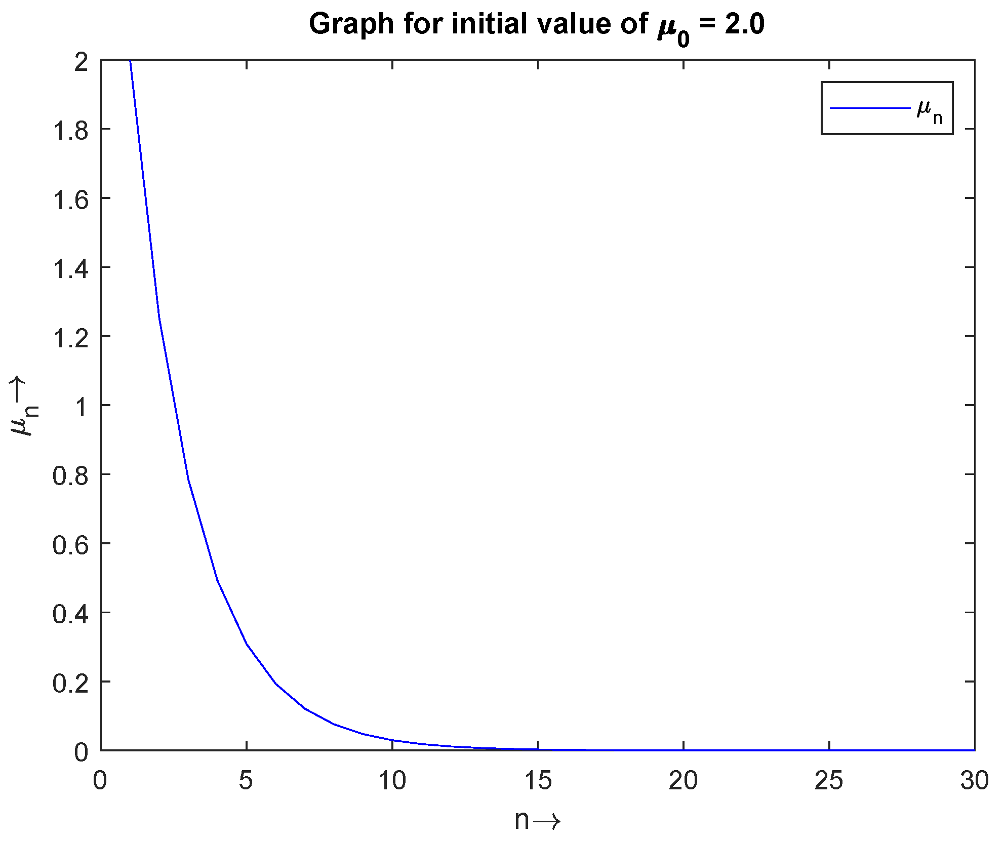
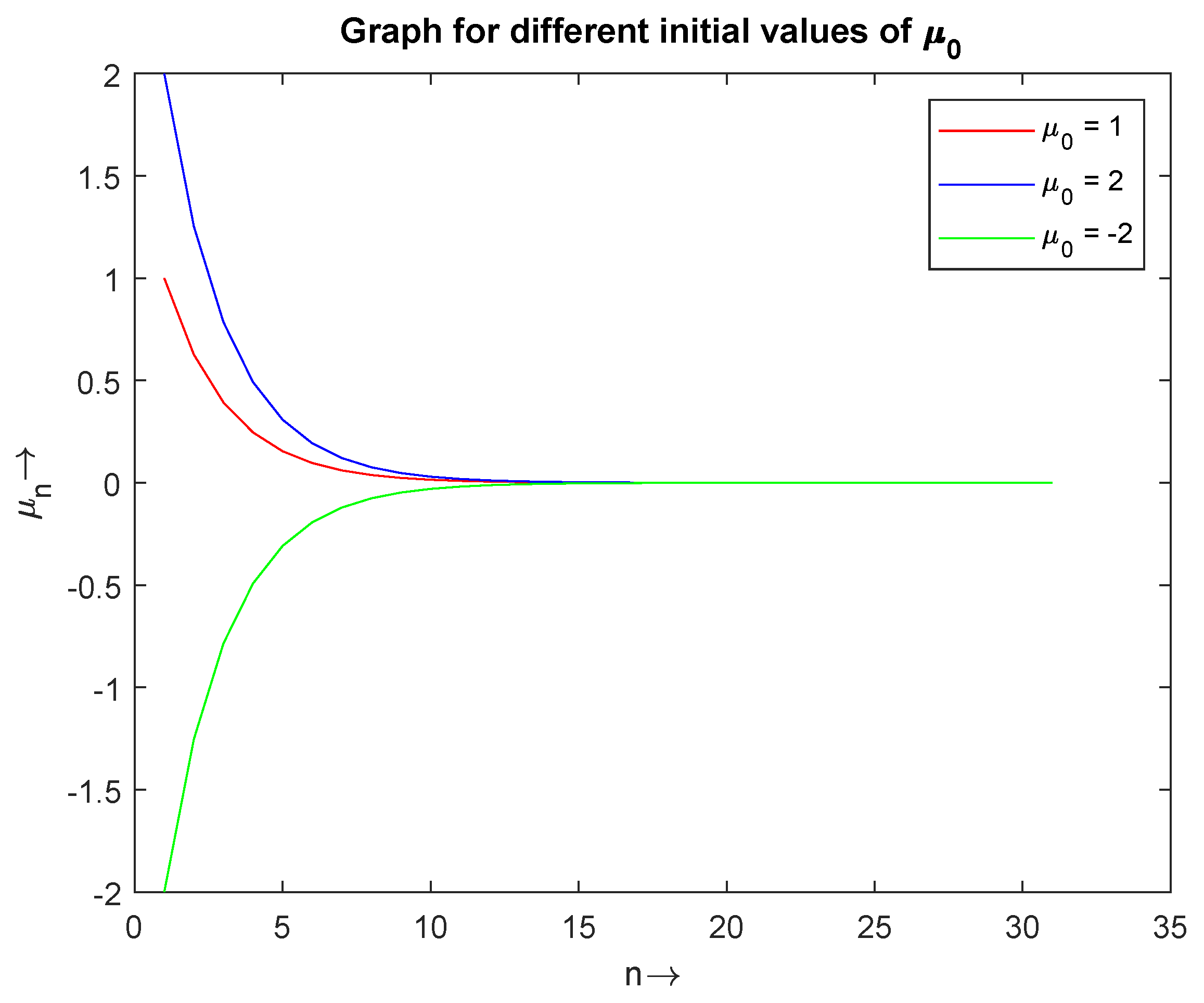
4. Numerical Example

We present the following numerical example using MATLAB, R2021a, to support our result.

Example 1.

Suppose $\Re =\mathbb{R}={\Re }^{*}$, $g:\mathbb{R}\to \mathbb{R}$ and $\eta :\mathbb{R}\times \mathbb{R}\to \mathbb{R}$ are the functions such that, $\forall \mu ,\nu \in \mathbb{R}$,

$$g\left(\mu \right)=\frac{3}{5}\mu ,$$

(18)

$$and\eta (\mu ,\nu )=\mu -\nu .$$

(19)

Clearly $\eta (\mu ,\nu )=-\eta (\nu ,\mu )$,

(i)

the function g is Lipschitz continuous with constant ${\lambda }_g=\frac{6}{5}$. i.e.,

$$\begin{array}{ccc}\hfill ∥g\left(\mu \right)-g\left(\nu \right)∥& =& ∥\frac{3}{5}\mu -\frac{3}{5}\nu ∥\hfill \\ & =& \frac{3}{5}∥\mu -\nu ∥\hfill \\ & \le & \frac{6}{5}∥\mu -\nu ∥.\hfill \end{array}$$

(20)

(ii)

Let $\psi :\mathbb{R}\to \mathbb{R}\cup \left\{+\infty \right\}$ be defined as

$$\psi \left(\mu \right)=2{\mu }^2\forall \mu \in \mathbb{R}.$$

(21)

Then, the η-subdifferential of ψ, which is, ${\partial }_{\eta }\psi \left(\mu \right)=4\mu$.

Now, for $\rho =1$, we compute the η-proximal operator and YAO:

$$\begin{array}{ccc}\hfill J_{\rho }^{{\partial }_{\eta }\psi }\left(\mu \right)& =& {\left[I+\rho {\partial }_{\eta }\psi \right]}^{-1}\left(\mu \right)\hfill \\ & =& {\left[I+4I\right]}^{-1}\left(\mu \right)\hfill \\ & =& {\left[5I\right]}^{-1}\left(\mu \right)\hfill \\ & =& \frac{1}{5}\mu ,\hfill \end{array}$$

(22)

and

$$\begin{array}{ccc}\hfill Y_{\rho }^{{\partial }_{\eta }\psi }\left(\mu \right)& =& \frac{1}{\rho }\left[I-J_{\rho }^{{\partial }_{\eta }\psi }\right]\left(\mu \right)\hfill \\ & =& \frac{1}{1}\left[\mu -\frac{1}{5}\mu \right]\hfill \\ & =& \frac{4}{5}\mu .\hfill \end{array}$$

(23)

Clearly, $J_{\rho }^{{\partial }_{\eta }\psi }$ is $\left(\frac{\tau }{\delta }\right)$-Lipschitz continuous, where $\delta =\tau =1$ and $Y_{\rho }^{{\partial }_{\eta }\psi }$ is ${\lambda }_Y$-Lipschitz continuous, where ${\lambda }_Y=\frac{\delta +\tau }{\rho \delta }=2$.

(iii)

$g\circ Y_{\rho }^{{\partial }_{\eta }\psi }$ is strongly accretive with constant ${\delta }_{gY}=\frac{1}{3}$. As

$$\begin{array}{ccc}\hfill g\circ Y_{\rho }^{{\partial }_{\eta }\psi }\left(\mu \right)& =& g\left(Y_{\rho }^{{\partial }_{\eta }\psi }\left(\mu \right)\right)\hfill \\ & =& g\left(\frac{4}{5}\mu \right)\hfill \\ & =& \frac{3}{5}\left(\frac{4}{5}\mu \right)\hfill \\ & =& \frac{12}{25}\mu ,\hfill \end{array}$$

(24)

therefore,

$$\begin{array}{ccc}\hfill 〈g\circ Y_{\rho }^{{\partial }_{\eta }\psi }\left(\mu \right)-g\circ Y_{\rho }^{{\partial }_{\eta }\psi }\left(\nu \right),\mu -\nu 〉& =& 〈\frac{12}{25}\mu -\frac{12}{25}\nu ,\mu -\nu 〉\hfill \\ & =& \frac{12}{25}〈\mu -\nu ,\mu -\nu 〉\hfill \\ & =& \frac{12}{25}{∥\mu -\nu ∥}^2\hfill \\ & \ge & \frac{1}{3}{∥\mu -\nu ∥}^2.\hfill \end{array}$$

(25)

(iv)

Let $P,Q,R:\mathbb{R}\to \mathbb{R}$ be the functions and $A,B,C:\mathbb{R}\to CB\left(\mathbb{R}\right)$ be the multivalued functions given by

$$P\left(\mu \right)=\frac{1}{4}\mu ,Q\left(\mu \right)=\frac{1}{5}\mu ,R\left(\mu \right)=\frac{4}{7}\mu$$

$$A\left(\mu \right)=\left\{\frac{1}{3}\mu \right\},B\left(\mu \right)=\left\{\frac{5}{4}\mu \right\},C\left(\mu \right)=\left\{\frac{1}{5}\mu \right\}.$$

Accordingly,

$$\begin{array}{c}\hfill {\xi }_n=\frac{1}{3}{\mu }_n\in A\left({\mu }_n\right)\\ \hfill {\vartheta }_n=\frac{5}{4}{\mu }_n\in B\left({\mu }_n\right)\\ \hfill and{\zeta }_n=\frac{1}{5}{\mu }_n\in C\left({\mu }_n\right),for alln=0,1,2,\dots .\end{array}$$

(26)

Using (14) of Algorithm 1 and by taking $\lambda =1$, we have

$$\begin{array}{ccc}\hfill {\mu }_{n+1}& =& {\mu }_n-g\left(Y_{\rho }^{{\partial }_{\eta }\psi }\left({\mu }_n\right)\right)+J_{\rho }^{{\partial }_{\eta }\psi }\left\{g\left(Y_{\rho }^{{\partial }_{\eta }\psi }\left({\mu }_n\right)\right)-\rho \left[P\left({\xi }_n\right)-\left(Q\left({\vartheta }_n\right)-R\left({\zeta }_n\right)\right)\right]\right\}\hfill \\ & =& {\mu }_n-\frac{12}{25}{\mu }_n+J_{\rho }^{{\partial }_{\eta }\psi }\left(\frac{12}{25}{\mu }_n-1\left[\frac{1}{12}{\mu }_n-\frac{1}{4}{\mu }_n+\frac{4}{35}{\mu }_n\right]\right)\hfill \\ & =& {\mu }_n-\frac{12}{25}{\mu }_n+J_{\rho }^{{\partial }_{\eta }\psi }\left(\frac{12}{25}{\mu }_n+\frac{11}{210}{\mu }_n\right)\hfill \\ & =& {\mu }_n-\frac{12}{25}{\mu }_n+J_{\rho }^{{\partial }_{\eta }\psi }\left(\frac{559}{1050}{\mu }_n\right)\hfill \\ & =& {\mu }_n-\frac{12}{25}{\mu }_n+\frac{1}{5}\left(\frac{559}{1050}{\mu }_n\right)\hfill \\ & =& {\mu }_n-\frac{12}{25}{\mu }_n+\frac{559}{5250}{\mu }_n\hfill \\ & =& \frac{3289}{5250}{\mu }_n.\hfill \end{array}$$

(27)

Figure 1, Figure 2 and Figure 3 (

Table 1. Computational results for different initial values of ${\mu }_0$.

No. of	${\mathit{\mu }}_0=1.0$	No. of	${\mathit{\mu }}_0=2.0$	No. of	${\mathit{\mu }}_0=-2.0$
Iterations	${\mathit{\mu }}_{\mathit{n}}$	Iterations	${\mathit{\mu }}_{\mathit{n}}$	Iterations	${\mathit{\mu }}_{\mathit{n}}$
1	1.0000	1	2.0000	1	−2.0000
2	0.6265	2	1.2530	2	−1.2530
3	0.3925	3	0.7850	3	−0.7850
4	0.2459	4	0.4918	4	−0.4918
5	0.1540	5	0.3081	5	−0.3081
6	0.0965	6	0.1930	6	−0.1930
7	0.0605	7	0.1209	7	−0.1209
8	0.0379	8	0.0757	8	−0.0757
9	0.0237	9	0.0474	9	−0.0474
10	0.0149	10	0.0296	10	−0.0296
14	0.0023	14	0.0045	14	−0.0045
18	0.0004	18	0.0007	18	−0.0007
22	0.0001	22	0.0001	22	−0.0001
26	0.0000	26	0.0000	26	0.0000
30	0.0000	30	0.0000	30	0.0000

) show the convergence of $\left\{{\mu }_n\right\}$ for the initial values ${\mu }_0=1,2$ and $-2$, respectively. In Figure 4, we have drawn a combine graph of $\left\{{\mu }_n\right\}$ for the initial values ${\mu }_0=1,2,-2$, and it is shown that the sequence $\left\{{\mu }_n\right\}$ converges to 0.

5. Conclusions

In order to establish the existence of the solution of (MVLIYAO), we find the equivalence between fixed point formulation and (MVLIYAO). Further, we proposed an iterative algorithm that is acquired from fixed point formulation to approximate the solution of (MVLIYAO). An existence and convergence result is obtained for (MVLIYAO) in Banach spaces. A numerical example is constructed to show the validity of our main result and the convergence graphs are presented using MATLAB programming. Furthermore, we mention that our results generalize the many existing results in the literature which can be extended to other spaces.

References

1. Baiocchi, C.; Capelo, A. Variational and Quasivariational Inequalities, Applications to Free Boundary Problems; Wiley: New York, NY, USA, 1984. [Google Scholar]
2. Giannessi, F.; Maugeri, A. Variational Inequalities and Network Equilibrium Problems; Plenum Press: New York, NY, USA, 1995. [Google Scholar]
3. Glowinski, R.; Lions, J.; Tremolieres, R. Numercial Analysis of Variational Inequalities; North-Holland: Amsterdam, The Netherlands, 1981. [Google Scholar]
4. Harker, P.T.; Pang, J.S. Finite-dimensional variational inequality and nonlinear complementarity problems. Math. Program. 1990, 48, 161–220. [Google Scholar] [CrossRef]
5. Kinderlehrer, D.; Stampacchia, G. An Introduction to Variational Inequalities and Their Applications; Academic Press: New York, NY, USA, 1980. [Google Scholar]
6. Hassouni, A.; Moudafi, A. A perturbed algorithm for variational inclusions. J. Math. Anal. Appl. 1994, 185, 706–712. [Google Scholar] [CrossRef] [Green Version]
7. Adly, S. Perturbed algorithms and sensitivity analysis for a general class of variational inclusions. J. Math. Anal. Appl. 1996, 201, 609–630. [Google Scholar] [CrossRef] [Green Version]
8. Huang, N.J. Generalized nonlinear variational inclusions with noncompact valued mappings. Appl. Math. Lett. 1996, 9, 25–29. [Google Scholar] [CrossRef] [Green Version]
9. Kazmi, K.R. Mann and Ishikawa perturbed iterative algorithms for generalized quasivariational inclusions. J. Math. Anal. Appl. 1997, 209, 572–584. [Google Scholar] [CrossRef] [Green Version]
10. Ding, X.P. Perturbed proximal point algorithms for generalized quasivariational inclusions. J. Math. Anal. Appl. 1997, 210, 88–101. [Google Scholar] [CrossRef] [Green Version]
11. Lescarret, C. Cas d‘addition des applications monotones maximales dans un espace de Hilbert. C. R. I‘Acadimic Sci. 1965, 261, 1160–1163. [Google Scholar]
12. Browder, F.E. On the unification of the calculus of variations and the theory of monotone nonlinear operators in Banach spaces. Proc. Natl. Acad. Sci. USA 1966, 56, 419–425. [Google Scholar] [CrossRef] [Green Version]
13. Konnov, I.V.; Volotskaya, E.O. Mixed variational inequalities and economic equilibrium problems. J. Appl. Math. 2002, 2, 289–314. [Google Scholar] [CrossRef] [Green Version]
14. Zarantonello, E.H. Solving Functional Equations by Contractive Averaging; Tech. Report 160; Mathematics Research Center, United States Army, University of Wisconsin: Madison, WI, USA, 1960. [Google Scholar]
15. Minty, G.J. Monotone (nonlinear) operators in Hilbert space. Duke Math. J. 1962, 29, 341–346. [Google Scholar] [CrossRef]
16. Ram, T.; Iqbal, M. Generalized monotone mappings with an application to variational inclusions. Commun. Math. Appl. 2022, 13, 477–491. [Google Scholar] [CrossRef]
17. Ahmad, R.; Ishtyak, M.; Rahaman, M.; Ahmad, I. Graph convergence and generalized Yosida approximation operator with an application. Math Sci. 2017, 11, 155–163. [Google Scholar] [CrossRef] [Green Version]
18. Cao, H.W. Yosida approximation equations technique for system of generalized set-valued variational inclusions. J. Inequal. Appl. 2013, 2013, 455. [Google Scholar] [CrossRef] [Green Version]
19. Lan, H.Y. Generalized Yosida approximations based on relatively A-maximal m-relaxed monotonicity frameworks. Abstr. Appl. Anal. 2013, 157190. [Google Scholar]
20. Qin, X.; Cho, S.Y.; Wang, L. A regularization method for treating zero points of the sum of two monotone operators. Fixed Point Theory Appl. 2014, 2014, 75. [Google Scholar] [CrossRef] [Green Version]
21. Ceng, L.C.; Wen, C.F.; Yao, Y. Iteration approaches to hierarchical variational inequalities for infinite nonexpansive mappings and finding zero points of m-accretive operators. J. Nonlinear Var. Anal. 2017, 1, 213–235. [Google Scholar]
22. Qin, X.; Petrusel, A.; Yao, J.C. CQ iterative algorithms for fixed points of nonexpansive mappings and split feasibility problems in Hilbert spaces. J. Nonlinar Convex Anal. 2018, 19, 251–264. [Google Scholar]
23. Rajpoot, A.K.; Ahmad, R.; Ishtyak, M.; Wen, C.-F. Mixed variational inequality problem involving generalized Yosida approximation operator in q-uniformly smooth banach space. J. Math. 2022, 2022, 5668372. [Google Scholar] [CrossRef]
24. Akram, M.; Chen, J.W.; Dilshad, M. Generalized Yosida approximation operator with an application to a system of Yosida inclusions. J. Nonlinear Funct. Anal. 2018, 2018, 17. [Google Scholar]
25. Penot, J.-P.; Ratsimahalo, R. On the Yosida approximaton of operators. Proc. R. Soc. Edinb. Math. 2001, 131, 945–966. [Google Scholar] [CrossRef]
26. Yu, Y. Convergence analysis of a Halpern type algorithm for accretive operators. Nonlinear Anal. 2012, 75, 5027–5031. [Google Scholar] [CrossRef]
27. Zeng, L.C.; Guu, S.M.; Yao, J.C. Characterization of H-monotone operators with applications to variational inclusions. Comput. Math. Appl. 2005, 50, 329–337. [Google Scholar] [CrossRef] [Green Version]
28. Ding, X.P.; Lou, C.L. Perturbed proximal point algorithms for general quasi-variational-like inclusions. J. Comput. Appl. Math. 2000, 113, 153–165. [Google Scholar] [CrossRef] [Green Version]
29. Verma, R.U. On generalized variational inequalities involving relaxed Lipschitz and relaxed monotone operators. J. Math. Anal. Appl. 1997, 213, 387–392. [Google Scholar] [CrossRef] [Green Version]
30. Lee, C.-H.; Ansari, Q.H.; Yao, J.-C. A perturbed algorithm for strongly nonlinear variational-like inclusions. Bull. Aust. Math. Soc. 2000, 62, 417–426. [Google Scholar] [CrossRef]
31. Ahmad, R.; Siddiqi, A.H.; Khan, Z. Proximal point algorithm for generalized multivalued nonlinear quasi-variational-like inclusions in Banach spaces. Appl. Math. Comput. 2005, 163, 295–308. [Google Scholar] [CrossRef]
32. Ahmad, R.; Siddiqi, A.H. Mixed variational-like inclusions and Jη-proximal operator equations in Banach spaces. J. Math. Anal. Appl. 2007, 327, 515–524. [Google Scholar] [CrossRef] [Green Version]
33. Nadler, S.B., Jr. Multi-valued contraction mappings. Pac. J. Math. 1969, 30, 475–488. [Google Scholar] [CrossRef] [Green Version]
Figure 1. The convergence of μ n with initial value μ 0 = 1 .
Mathematics 10 04067 g001
Figure 2. The convergence of μ n with initial value μ 0 = 2 .
Mathematics 10 04067 g002
Figure 3. The convergence of μ n with initial value μ 0 = 2 .
Mathematics 10 04067 g003
Figure 4. The convergence of μ n with initial values μ 0 = 1 , μ 0 = 2 and μ 0 = 2 . .
Mathematics 10 04067 g004