Article

A Q-Learning and Fuzzy Logic-Based Hierarchical Routing Scheme in the Intelligent Transportation System for Smart Cities

by
Amir Masoud Rahmani
1,†,
Rizwan Ali Naqvi
2,†,
Efat Yousefpoor
3,
Mohammad Sadegh Yousefpoor
3,
Omed Hassan Ahmed
4,
Mehdi Hosseinzadeh
5,* and
Kamran Siddique
6,7,*
1
Future Technology Research Center, National Yunlin University of Science and Technology, Yunlin, Douliou 64002, Taiwan
2
School of Intelligent Mechatronics Engineering, Sejong University, Seoul 05006, Korea
3
Department of Computer Engineering, Dezful Branch, Islamic Azad University, Dezful 5716963896, Iran
4
Department of Information Technology, University of Human Development, Sulaymaniyah 0778-6, Iraq
5
Pattern Recognition and Machine Learning Lab, Gachon University, 1342 Seongnamdaero, Sujeonggu, Seongnam 13120, Korea
6
Department of Information and Communication Technology, School of Computing and Data Science, Xiamen University Malaysia, Sepang 43900, Malaysia
7
Department of Computer Science and Engineering, University of Alaska Anchorage, Anchorage, AK 99508, USA
*
Authors to whom correspondence should be addressed.
These authors contributed equally to this work.
Mathematics 2022, 10(22), 4192; https://doi.org/10.3390/math10224192
Submission received: 5 October 2022 / Revised: 27 October 2022 / Accepted: 1 November 2022 / Published: 9 November 2022

Abstract

:
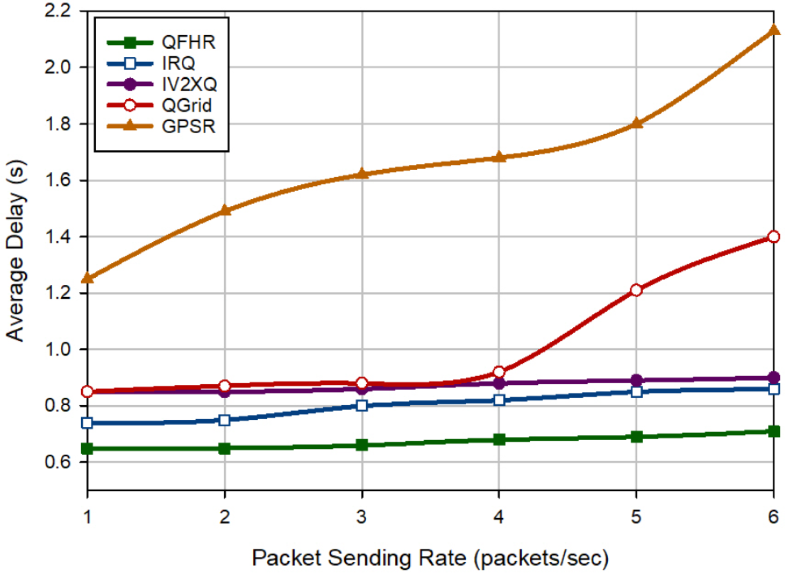
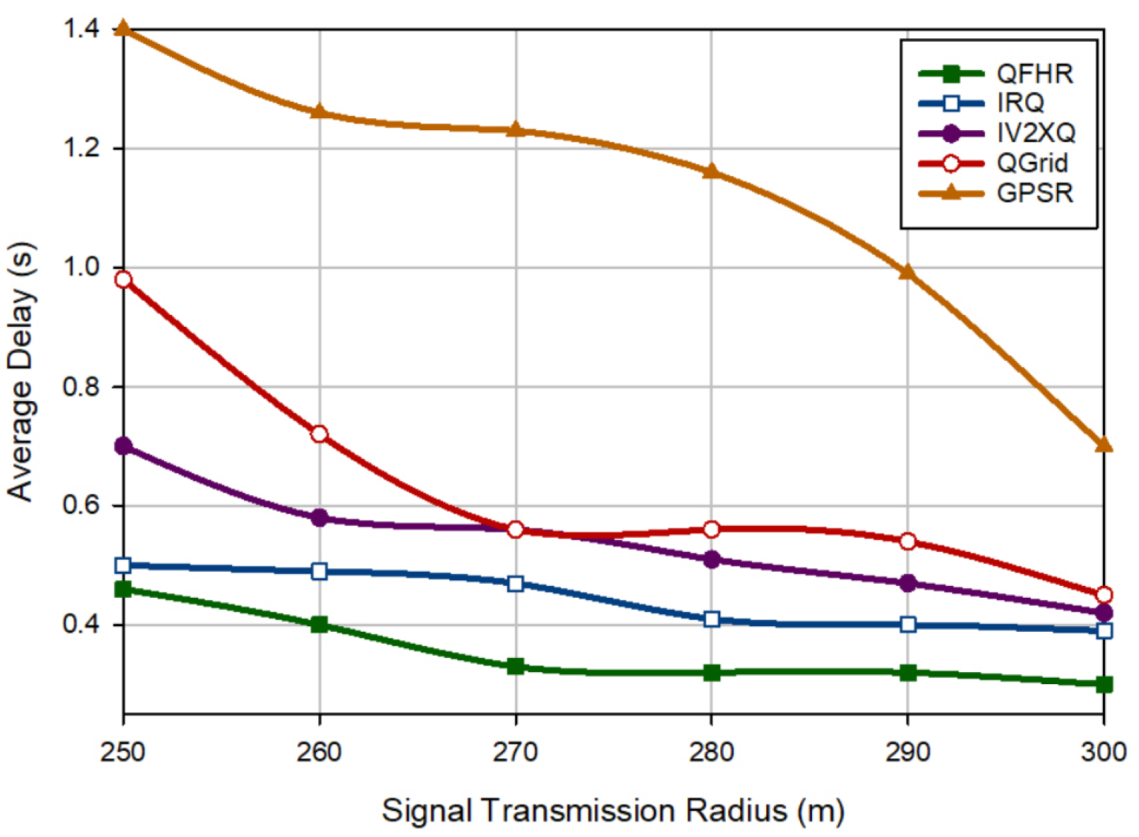
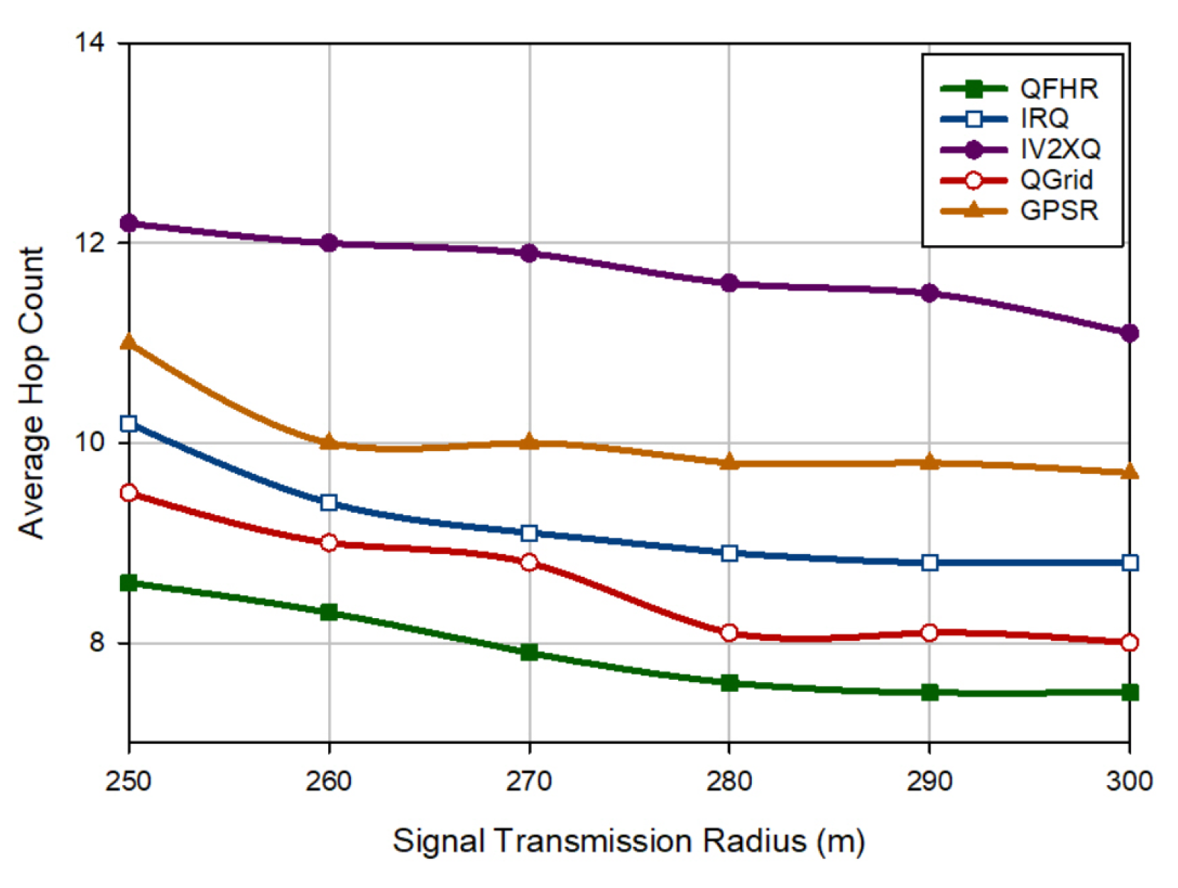
A vehicular ad hoc network (VANET) is the major element of the intelligent transportation system (ITS). The purpose of ITS is to increase road safety and manage the movement of vehicles. ITS is known as one of the main components of smart cities. As a result, there are critical challenges such as routing in these networks. Recently, many scholars have worked on this challenge in VANET. They have used machine learning techniques to learn the routing proceeding in the networks adaptively and independently. In this paper, a Q-learning and fuzzy logic-based hierarchical routing protocol (QFHR) is proposed for VANETs. This hierarchical routing technique consists of three main phases: identifying traffic conditions, routing algorithm at the intersection level, and routing algorithm at the road level. In the first phase, each roadside unit (RSU) stores a traffic table, which includes information about the traffic conditions related to four road sections connected to the corresponding intersection. Then, RSUs use a Q-learning-based routing method to discover the best path between different intersections. Finally, vehicles in each road section use a fuzzy logic-based routing technique to choose the foremost relay node. The simulation of QFHR has been executed on the network simulator version 2 (NS2), and its results have been presented in comparison with IRQ, IV2XQ, QGrid, and GPSR in two scenarios. The first scenario analyzes the result based on the packet sending rate (PSR). In this scenario, QFHR gets better the packet delivery rate by 2.74%, 6.67%, 22.35%, and 29.98% and decreases delay by 16.19%, 22.82%, 34.15%, and 59.51%, and lowers the number of hops by 6.74%, 20.09%, 2.68%, and 12.22% compared to IRQ, IV2XQ, QGrid, and GPSR, respectively. However, it increases the overhead by approximately 9.36% and 11.34% compared to IRQ and IV2XQ, respectively. Moreover, the second scenario evaluates the results with regard to the signal transmission radius (STR). In this scenario, QFHR increases PDR by 3.45%, 8%, 23.29%, and 26.17% and decreases delay by 19.86%, 34.26%, 44.09%, and 68.39% and reduces the number of hops by 14.13%, 32.58%, 7.71%, and 21.39% compared to IRQ, IV2XQ, QGrid, and GPSR, respectively. However, it has higher overhead than IRQ (11.26%) and IV2XQ (25%).

1. Introduction

There is a great demand for vehicular ad hoc networks in which vehicles can communicate with each other without any infrastructure. The purpose of these networks is to reduce delays in traffic flow and improve driving quality. These networks have attracted the attention of universities and industries because they can improve road safety and provide many services to drivers and travelers. VANET is the core of an intelligent transportation system (ITS) [1,2]. It does not require an expensive infrastructure because wireless technology is cheap and ubiquitous. In VANET, when vehicles have a direct connection with each other, they create a vehicle-to-vehicle (V2V) connection. When vehicles interact with roadside units (RSUs), they form a vehicle-to-infrastructure (V2I) connection. Over the past decade, researchers have introduced various methodologies to provide better routing techniques in VANET to avoid road accidents. For example, a vehicle can help other drivers and inform them of an unexpected position so that drivers take appropriate action in response to this event. This attractive feature is very important for making smart cities [3,4]. View Figure 1. The smart city has no certain definition in the world. However, the motivation to build such a city in different countries is to improve physical, social, and economic infrastructure. In fact, a smart city is created when the city efficiently presents public services provided by the government, increases the quality of services for citizens, and reduces government costs. These programs will not only improve the life quality of citizens but also lead to financial interests for the economy. Today, deploying a smart city requires a safe road that includes road conditions, good mobility, vehicle safety, and easy access to the Internet to provide drivers/passengers services and comfort [5,6].
Routing is a process for transferring packets between source and destination. In VANET, routing depends on some factors, for example velocity, density, and movement direction [7,8]. As a result, a challenging problem is to design a routing approach in vehicular ad hoc networks. Thus, traditional routing protocols should be updated for the dynamic environment of VANET [9,10]. When designing routing protocols in VANETs, some routing challenges include high dynamic topology, frequent disconnections, mobility model, propagation model, communication environment, delay constraint, and quality of service (QoS) requirements. Routing protocols in VANET are categorized as follows: topology-based [11,12], geographic [12], hybrid [6,13], clustering-based [6,14], opportunistic [6,14], and data fusion [11,14].
Recently, many scholars are working on the routing challenge in VANET. They have used machine learning (ML) techniques to address the routing challenge in VANET adaptively and independently [15,16]. Reinforcement learning (RL) is the most efficient ML techniques for deploying routing algorithms in VANET. This algorithm is popular due to the trial and error technique [17,18]. In reinforcement learning-based routing, the agent discovers the network by taking different actions to earn a routing policy [19,20]. To achieve this goal, the agent must search for the best path in accordance with several criteria, which are obtained from local information of nodes to reduce energy consumption and improve network connections. However, in order to achieve an optimized routing technique, the agent requires global information about the entire system.
In this paper, a Q-learning and fuzzy logic-based hierarchical routing algorithm (QFHR) is proposed in VANETs. In the method, the focus is on delay reduction in the routing process. QFHR utilizes a hierarchical routing technique. In this scheme, RSUs use a Q-learning-based routing operation to discover paths between different intersections in the urban environment. In the existing Q-learning-based routing algorithms, researchers often consider vehicles as the state space in Q-learning. Therefore, when increasing the density of vehicles, the state space is dramatically increased in the routing algorithm. This affects the convergence speed of this algorithm negatively. Therefore, QFHR considers intersections as the state set to manage the convergence speed of the routing algorithm. On the other hand, vehicles in each road segment use a fuzzy logic-based greedy routing technique to choose the most suitable next-hop node. As a result, the main contributions of our work are as follows:
  • In QFHR, a traffic detection algorithm is presented for identifying the traffic status of four road sections connected to each intersection. The algorithm provides new traffic information for the Q-learning-based routing process and inform RSUs of the traffic status in the network at any moment.
  • In QFHR, a Q-learning-based routing scheme called the intersection-to-intersection (I2I) routing algorithm is designed in accordance with a distributed strategy to obtain the best route between different intersections using traffic information. Moreover, The I2I routing algorithm manages network congestion and can quickly discover and replace congested paths.
  • In QFHR, a greedy routing technique is designed by vehicles to find the best route in each road section. This algorithm addresses the local optimum issue using a fuzzy path recovery algorithm.
In the following, the paper is organized as follows: Section 2 demonstrates the related works. Section 3 explains reinforcement learning algorithms, especially Q-learning and fuzzy logic because the proposed method utilizes these techniques for designing the routing process. Section 4 introduces the network system applied in QFHR. Section 5 describes QFHR in VANETs. In Section 6 evaluates the performance of QFHR based on packet delivery rate, end-to-end delay, hop count, and routing overhead. Ultimately, Section 7 presents the conclusions of our paper.

2. Related Works

Sun et al. [21] have presented a position-based Q-learning routing (PbQR) scheme for VANET. In this method, reliability and link stability are considered to choose relay nodes in the data transmission operation. PbQR regards vehicles as the state set in the learning algorithm. In this scheme, Hello messages are periodically exchanged between neighboring nodes to share their information. PbQR applies Q-learning in the routing process. Thus, the agent always takes a greedy action, meaning that it always chooses the most suitable action, which is available in Q-table. PbQR evaluates link quality based on two factors, namely stability and continuity to choose the next-hop node. The continuity factor is defined based on node degree. In this method, the reward function is equal to the sum of these factors in each node. PbQR defines a distance factor to specify the distance from source to destination. In Q-learning, the discount factor is implemented based on the distance factor.
Roh et al. [22] have offered the Q-learning-based load balancing routing (Q-LBR) protocol in VANETs. It is a UAV-assisted routing protocol. Thus, it provides line-of-sight (LOS) communications for ground vehicles. Q-LBR utilizes three mechanisms to balance the load in the network. In the first mechanism, the authors have suggested an optimized load estimation for ground vehicles. In this technique, ground vehicles disseminate hello messages to transfer their buffer queue information to UAVs. In the second mechanism, Q-learning is used to establish communication paths using a load-balancing manner. To achieve this end, it defines a new concept called the UAV routing policy area (URPA). Ultimately, the authors try to define a reward function that accelerates the convergence speed related to the learning model. This approach introduces different packets for three types of services, namely emergency, real-time, and connection-oriented. These messages have various priorities, including high, medium, and low. Q-LBR involves two sections. In the first section, UAV hears broadcast messages to collect the congestion conditions in the ground vehicles. Then, it detects the congestion level in the ground network. URPA information is broadcast in the second section. Q-LBR discovers paths similar to AODV and DSR. It supports multipath routing. Thus, it can manage the number of routing messages exchanged between nodes in the network.
Bi et al. [23] have introduced the reinforcement learning-based routing protocol in clustered networks (RLRC) for electric vehicles. RLRC utilizes a clustering process to divide the network into several clusters. RLRC uses an enhanced K-Harmonic Means (KHM) for the clustering process and considers two factors, namely the energy of vehicles and bandwidth when selecting the best cluster head (CH). KHM is another version of the K-Means clustering method. This scheme considers the harmonic mean as an alternative option instead of the minimum value. In the first step, it calculates partial derivatives to achieve the best position for the centroid. In each iteration, the algorithm improves the centroid. The clustering algorithm considers the relative distance to select CHs based on the least distance to the neighbors. Non-CH nodes calculate the distance between themselves and CHs and join the nearest CH. To reduce learning time, RLRC utilizes the state-action-reward-state-action (SARSA) algorithm to enhance the routing process. It regards the clustered network as the learning environment, and CHs play the agent role. In RLRC, Hello messages are disseminated in the network to refresh Q-values. In the learning algorithm, the reward function is defined with regard to the next-hop link state. It considers three scales, including hop count, link condition, and available bandwidth for calculating Q-values.
Yang et al. [24] have offered the heuristic Q-learning-based VANET routing (HQVR) protocol. It selects the intermediate vehicles based on link reliability. This scheme uses a distributed manner to implement the learning process based on the information extracted from beacon messages. However, the authors have not taken into account the road width. In this method, the convergence speed of the Q-learning algorithm is dependent on the beacon packet rate. HQVR considers the link lifetime as the learning rate to determine the convergence speed of the learning protocol. HQVR has a route discovery strategy, which depends on delay information. When a node compares the new path and the old path in terms of delay and realizes that the new path requires less time than the previous path, it switches to the new path. Feedback messages find several routes to the destination. As a result, the source vehicle chooses the best route among different paths.
Wu et al. [25] have offered the Q-learning-based VANET delay-tolerant routing protocol (QVDRP) for VANET. This method uses several gateways to transfer data from source to destination. In this method, RSUs play the gateway role to communicate with the cloud server. In QVDRP, vehicles disseminate their generated data to RSUs. This reduces delay and maximizes packet delivery rate when transferring data from a node to another. In QVDRP, the network is regarded as the learning system, and vehicles play the agent role. In the learning operation, data is exchanged between nodes to select the next action (i.e., the next-hop node). Each vehicle stores a Q-table, which involves Q-values of other vehicles. In the learning operation, vehicles disseminate hello messages to refresh Q-table. If the transmitter vehicle and the destination vehicle form a direct connection with each other, this link receives a positive reward. If the previous-hop node receives a message from another node after a threshold time, they obtain a discounted reward. Otherwise, its default reward is adjusted to 0.75. QVDRP predicts the input and output directions in each road segment to obtain a collision probability to reduce the duplicated packets.
Karp and Kung in [26] have designed the greedy perimeter stateless routing (GPSR) in ad hoc networks. The greedy routing strategy utilizes the local information of single-hop neighboring vehicles to deliver data packets through the nearest node to the destination. GPSR is a position-based routing approach, which merges greedy and perimeter strategies. It refreshes the neighbor table by exchanging beacon messages that increase routing overhead. However, it has an acceptable routing overhead and delay. GPSR deals with some limitations in the routing process in VANET because it ignores parameters such as delay, node speed, and movement direction.
Li et al. in [27] have suggested the Q-learning and grid-based routing protocol (QGrid) for VANETs. This protocol divides the network environment into several grids. Then, the Q-learning algorithm learns traffic flow to select the optimal grid based on Q-values. In each grid, the relay node is selected based on two techniques namely the greedy method and the second-order Markov chain prediction technique. In QGrid, the packet delivery issue from a vehicle to a fixed destination is investigated. In the routing process between different grids, a set of grids with the maximum Q-value is chosen. When increasing the number of packets on the network, this method has not suggested any mechanism for controlling network congestion. In addition, intersections and buildings may disrupt the data transfer process in urban areas. However, this issue has not been addressed in QGrid. Moreover, this method designs an off-line Q-table, which is fixed throughout the simulation process. Thus, QGrid cannot control the network load.
Lou et al. in [28] have suggested the intersection-based V2X routing via Q-learning (IV2XQ) for VANET. This hierarchical routing scheme uses a Q-learning-based routing algorithm at the intersection level to select the best routes between intersections. In IV2XQ, road intersections are regarded as the state space, and the road segments are considered as the action space. Thus, IV2XQ reduces the number of states in the Q-learning algorithm and improves its convergence speed. Moreover, vehicles use a greedy technique to choose the relay node based on the positions of vehicles in the road segments. In addition, one important task of RSUs is to monitor the network status to control congestion in the network. IV2XQ does not use any control packet for finding routes. Thus, it has low routing overhead and delay because IV2XQ only uses historical traffic information in the reinforcement learning-based routing process. However, it is very important to consider new information in the routing decisions.
Khan et al. in [29] have presented an intersection-based routing method using Q-learning (IRQ) in VANETs. This scheme defines two global and local views and proposes a traffic dissemination mechanism to create these views. This mechanism helps IRQ to update traffic information and provide a new and fresh global view for the network server. The global view is used for designing a Q-learning-based routing technique. This RL-based routing method finds the best routes between intersections and is executed by the central server. In the Q-leaning algorithm, the discount factor is determined dynamically based on distance and vehicle density in each road section. Thus, IRQ is compatible with the dynamic environment of VANET. IRQ introduces an evaluation mechanism to detect and penalize congested paths. This improves the packet delivery rate. The local view is used for designing a greedy routing strategy on each road segment to discover the best next-hop node. It considers the vehicle status, including location, distance, connection time, and delay.
Table 1 expresses briefly the strengths and weaknesses of the related works.

3. Base Concepts

In this section, two techniques, namely the Q-learning algorithm and the fuzzy logic, are briefly explained because QFHR uses these techniques to find the best route in the data transmission process in VANET.

3.1. Reinforcement Learning

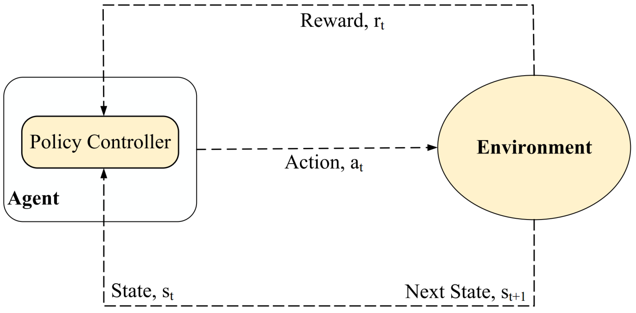
In artificial intelligence (AI), there is an important and useful tool called reinforcement learning (RL), which defines two main components, agent and environment. The agent chooses an action to interact with the environment. The aim of this interaction is to achieve an optimal solution for a certain issue. RL supports a specific framework called the Markov decision process (MDP) for solving optimization issues [30,31]. MDP manages the optimization problem using a random manner and defines four parameters such as S , A , p , r . The first parameter is S and indicates the finite state space. The second parameter (i.e., A) is the finite action space. The third parameter (i.e., P) represents the transition function. This function determines the next state s after doing the action a in the current state s. The last parameter is r, which indicates the reward function in the learning issue. This function determines the reward obtained from the learning environment after taking the action a t by the agent in the state s t . Note that t indicates time. Figure 2 displays reinforcement learning. In this process, the agent searches the environment by taking the action a t in the current state s t . Now, the environment calculates the reward value (r) and the next state s t + 1 by considering the performed action and the current state. The purpose of this learning framework is to reach the most suitable policy π and achieve the maximum reward. The long-term purpose of the agent is to boost the expected discounted reward (i.e., max t = 0 T δ r t s t , π s t ). δ illustrates the discount factor and indicates the effect of the reward on the Q-value. It is adjustable in 0 , 1 . If δ = 1 , the agent is only dependent on previous experiences. In contrast, if δ = 0 , the agent considers only the last immediate reward received from the environment [30,31]. After determining reward values and transition probabilities, the Q-value is obtained from the Bellman function presented in Equation (1):
Q s t , a t = 1 α Q s t , a t + α r + δ max Q s t + 1 , a t
In the Bellman equation, α is the learning rate. It is adjustable in 0 , 1 and creates a tradeoff between exploration and exploitation. It determines whether the agent focuses on new or old information. If α = 0 , the agent does not learn any new knowledge, and if α = 1 , the agent only regards the last information.
The most efficient RL technique is Q-learning. In this technique, the agent explores an unknown environment using a trial and error technique. In this method, the agent stores a Q-table, which includes the optimal state-action pairs and corresponding Q-values. The Q-learning algorithm must maximize Q-value by adjusting the action selection process in accordance to the reward received from the environment and evaluating the selected action in the current state. In each iteration, the Q-learning algorithm refreshes Q-values according to Equation (1). Next, the agent exploits the environment and selects actions with maximum Q-value. This scheme is called ϵ -greedy, which defines a probability value ( ϵ ) for the exploration or exploitation processes [32,33].

3.2. Fuzzy Logic

Researchers’ studies show that real and complicated processes cannot be modeled, measured, or managed accurately because they include various uncertainties such as uncompleted data, random data, noise data, outliers, and data loss. A robust solution for solving this issue is to use a useful mathematical technique called fuzzy logic (FL). It can describe human thinking in an approximate manner. Zadeh first introduced this theory in 1965. Note that the classical set theory presents a precise and certain definition of membership. Based on this definition, an element either belongs to a set or not. In contrast, the fuzzy theory emphasizes a novel concept called partial membership [34,35]. According to this concept, an element may partly be belonging to a set. Thus, the results are not right or wrong absolutely.
In the fuzzy theory, assume that X indicates a reference set, which includes a set of elements such as x. In this mode, Equation (2) defines the fuzzy set (i.e., A) based on X.
A = { ( x , μ A ( x ) ) | x X } = i = 1 n μ A ( x i ) / x i
where, μ A : X 0 , 1 means the membership function (MF). It determines the membership degree (i.e., μ A ( x i ) ) for each element (i.e., x) in A. “/” is a symbol for separating μ A ( x i ) from x. Note that MF is a key component in fuzzy sets. For example, the triangular function, trapezoidal function, and Gaussian function are known as the most common MFs.
Today, various applications utilize fuzzy inference mechanisms (FIMs) to improve their performance. The most famous FIMs are Mamdani and Sugeno (TSK). In each fuzzy system, there are four main parts, including the fuzzifier, defuzzifier, rule base, and fuzzy engine. The fuzzifier produces fuzzy inputs based on crisp values and allocates a membership degree to each element using the defined membership functions. The fuzzy engine uses fuzzy rules stored in the rule base to simulate fuzzy inputs. Finally, the results obtained from the fuzzy engine are converted to crisp values using the defuzzifier. The most common defuzzification techniques are averaging and centroid [35,36].

4. Network Model

In QFHR, the network environment consists of various intersections, which are connected to one another through two-way roads. Furthermore, QFHR defines both communication links namely vehicle-to-vehicle (V2V) and vehicle-to-infrastructure (V2I). Network elements, like road sections, intersections, roadside units (RSUs), and vehicles have a unique ID. Figure 3 displays this network model. In the following, the task of vehicles and RSUs in the network is explained:
  • Roadside units (RSUs): These components are located at intersections, and their task is to monitor the network and control congestion in each road section. RSUs store a traffic table to record the traffic status of the four road sections connected to the corresponding intersection. This table is periodically updated. Moreover, each RSU holds a Q-table produced by the Q-learning-based routing algorithm to select the best routes between different intersections on the network.
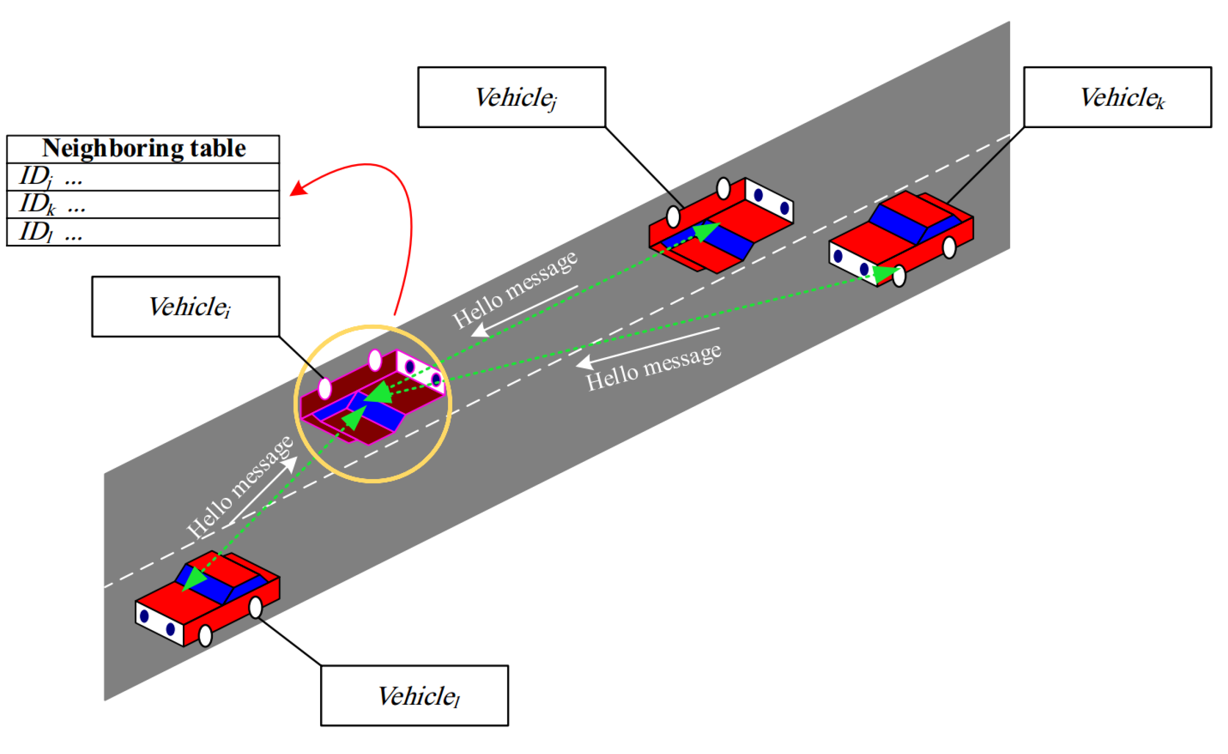
  • Vehicles: Each vehicle periodically sends a hello message to its neighboring nodes. These vehicles establish a neighbor table in their memory to store information about neighboring nodes. Additionally, they can achieve their position and speed at any time using a positioning system.

5. Proposed Method

In this paper, a Q-learning and fuzzy logic-based hierarchical routing method (QFHR) is proposed in vehicular ad hoc networks. At each intersection, RSUs use a Q-learning-based routing algorithm to obtain the most suitable path between different intersections on the network. Furthermore, vehicles use a fuzzy logic-based routing technique to find the next relay in each road section. QFHR consists of three main phases:
  • Identifying traffic conditions;
  • Routing algorithm at the intersection level;
  • Routing algorithm at the road section level.

5.1. Identifying Traffic Conditions

For knowing traffic conditions in each road section, QFHR presents a traffic detection process in the network. Algorithm 1 offers a pseudo-code for identifying traffic conditions in QFHR. In this process, each vehicle (such as V e h i c l e i , where i = 1 , 2 , . . . , N and N represent the number of vehicles) disseminates a hello packet to the neighbors periodically. In QFHR, the hello broadcast time ( τ ) is equal to one second. The hello message includes vehicle ID ( I D i ), road ID ( I D R ), queue status ( Q i ), vehicle location x i , y i , and vehicle speed v x , i , v y , i . Note that the vehicle speed is unchanged at the timeframe τ and is updated after receiving each hello message. V e h i c l e i builds a neighbor table ( T a b l e n e i g h b o r i ) to record the information about neighboring nodes. This operation is represented in Figure 4. If V e h i c l e i receives a new hello packet, it searches the ID related to the packet in its neighbor table. If this ID is in the table, V e h i c l e i updates the recorded information about this vehicle in its neighbor table. Otherwise, it adds a new entry to this table and records the information about the new vehicle. Table 2 shows the format of the neighbor table. In the following, various fields of the table are explained:
  • Vehicle ID: This field represents the identification of a neighboring vehicle in the road section. After receiving a hello packet from a neighbors, V e h i c l e i searches its ID in its neighbor table. If this ID is not available in the table, it adds a new entry to this table and records this ID in the ”Vehicle ID” field.
  • Road ID: This field is the identification of the road section corresponding to the neighboring vehicle. Upon receiving a new hello message, V e h i c l e i refreshes the road ID corresponding to the vehicle recorded in its neighbor table.
  • Spatial coordinates: It indicates the position of a neighboring vehicle in the road section and is updated after the time period τ .
  • Speed: This field indicates the speed of the neighboring vehicle in the road section. It is fixed at the time period τ and refreshed after receiving the new hello message.
  • Queue status: Using this parameter, V e h i c l e i can detect the congestion level in the neighboring vehicle. The queue status ( Q j ) is normalized using Equation (3).
    Q j = Q L j max Q L j
    where, Q L j and max Q L j are the number of packets in the queue and maximum queue length of V e h i c l e j , respectively.
  • Connection quality: It represents the quality of the connection between V e h i c l e i and V e h i c l e j . It is measured based on two parameters, namely the connection time and the hello packet reception rate. Section 5.1.1 describes how to calculate this parameter in detail.
  • Validity time: It is a time interval when this entry is valid in the neighbor table. After receiving each new hello message from a vehicle, this time interval is refreshed. If the new hello message is not received from the vehicle, the entry related to the vehicle will be removed from the neighbor table after ending the validity time.

5.1.1. Calculating the Connection Quality of Two Vehicles

In QFHR, the quality of the connection between V e h i c l e i and V e h i c l e j , namely C Q i , j , is evaluated with regard to two factors, namely the connection time and the hello packet reception rate because the connection time indicates the stability of the link between the two nodes and the packet reception rate also evaluates their connection quality. It is difficult to calculate the connection quality because the nodes are mobile. In the proposed method, C Q i , j is obtained from the weighted mean of two parameters, including the connection time of V e h i c l e i and V e h i c l e j (i.e., λ i j ) and the hello packet reception rate (i.e., η i j ) based on Equation (4):
C Q i , j = ω 1 λ i j + 1 ω 1 η i j V e h i c l e j N e i g h b o r i ω 1 λ i j + 1 ω 1 η i j
So, N e i g h b o r i represents the neighbors of V e h i c l e i . Moreover, ω 1 is a weight coefficient and 0 ω 1 1 .
In the following, we demonstrate how to obtain the connection time ( λ i j ) and the hello reception rate ( η i j ).
  • Connection time ( λ i j ): The connection time of V e h i c l e i and V e h i c l e j is evaluated by Equation (5):
    λ i j = R d i j Δ V i j T max
    where, R is the communication radius of vehicles, d i j = x i x j 2 + y i y j 2 is the Euclidean distance between the two vehicles and Δ V i j = v i v j expresses the relative speed of V e h i c l e j with regard to V e h i c l e i . Moreover, x i , y i and x j , y j represent the spatial coordinates of V e h i c l e i and V e h i c l e j , respectively. In addition, v i and v j are their speed. T max is the maximum connection time, which is a fixed value determined based on the simulation time. To accurately estimate the connection time in the dynamic environment of VANET, two configuration coefficients are added to Equation (6). As a result:
    λ i j = R α 1 d i j v i α 2 v j T max
    where, α 1 and α 2 are the configuration coefficients that are determined as follows:
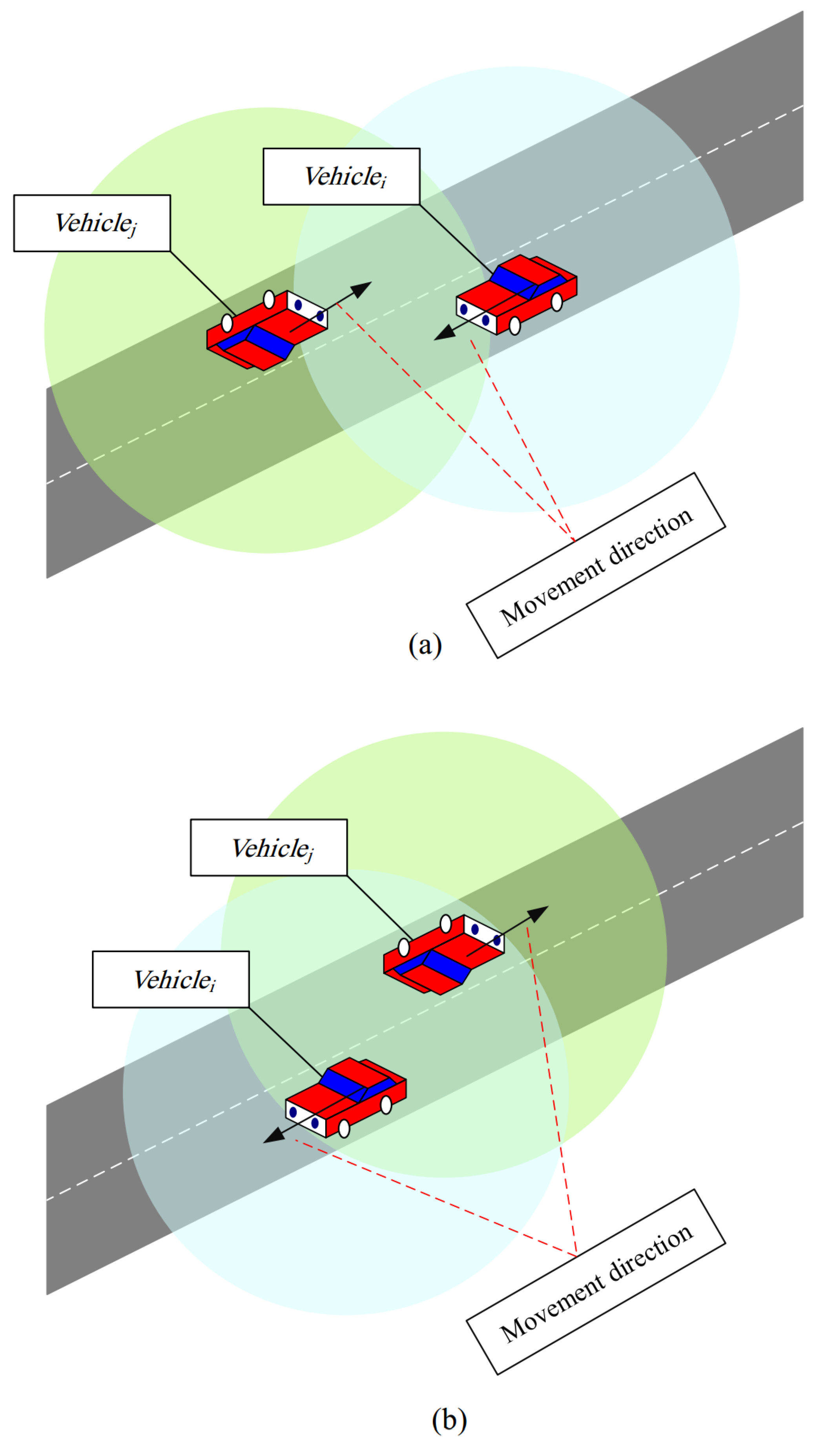
  • If V e h i c l e i and V e h i c l e j move at a similar direction (i.e., 0 Δ θ i j π 3 , so that Δ θ i j is the movement direction of V e h i c l e j with regard to V e h i c l e i ), then α 2 = 1 . Now if V e h i c l e i is ahead of V e h i c l e j , then α 1 = 1 . Otherwise, α 1 = 1 . See Figure 5.
  • If V e h i c l e i and V e h i c l e j move in the opposite direction (i.e., 2 π 3 Δ θ i j π ) then, α 2 = 1 . Now, if V e h i c l e i approaches V e h i c l e j , then α 1 = 1 . Otherwise, α 1 = 1 . See Figure 6.
In addition, Δ θ i j is obtained from Equation (7):
Δ θ i j = cos 1 v x , i v x , j + v y , i v y , j v x , i 2 + v y , i 2 × v x , j 2 + v y , j 2 , 0 Δ θ i j π
where v x , i , v y , i and v x , j , v y , j are the velocity vectors of V e h i c l e i and V e h i c l e j , respectively.
Then, each vehicle updates the connection time ( λ i j ) using the approach of window mean with exponentially weighted moving average (WMEWMA).
WMEWMA is an EWMA-based estimator that approximates the average value. It uses the linear combination of a limited exponentially weighed history [37,38]. Equation (8) is used to calculate this estimation recursively:
W M E W M A t = β W M E W M A t 1 + 1 β X t
where X t is the value of X at the moment t. Note that Equation (8) can be rewritten as Equation (9):
X l = β k = t L w i n d o w t 1 X k L w i n d o w + 1 β X t
WMEWMA has two control parameters, namely window size ( L w i n d o w ) and the control coefficient β so that 0 β 1 . Each window records the last L w i n d o w values. When β has a higher value, this estimation is more dependent on historical values. This means that the estimation is more stable. In contrast, if β = 0 , the average value depends only on the last value. This scale can create a stable estimation and is calculated easily.
  • Hello packet reception rate ( η i j ): The quality of the link between V e h i c l e i and V e h i c l e j is measured based on the ratio of the hello packages received by V e h i c l e i to all hello packets transmitted by V e h i c l e j at the time interval Φ . Each node uses a counter to count the number of hello messages received from its neighbors. Moreover, the hello broadcast time is equal to the specified time frame τ . As a result, the number of hello messages sent by V e h i c l e j can be calculated in a certain time Φ . Therefore, each vehicle can calculate the hello reception rate according to Equation (10):
    η i j = t Φ R h e l l o i , j t Φ S h e l l o i , j
    where R h e l l o i , j and S h e l l o i , j are equal to the number of received hello messages and the number of sent hello messages, respectively. Then, each vehicle uses Equation (9) to refresh the hello reception rate ( η i j ) using the WMEWMA method.

5.1.2. Forming a Traffic Table

To know the network status, each RSU holds two tables in its memory. In the following, each table is demonstrated exactly.
  • Neighbor table ( Table neighbor ): It contains information about neighboring vehicles. The format of this table is presented in Section 5.1. After receiving new hello messages from vehicles in different road sections, RSU searches their IDs in its neighbor table. If these IDs are in the table, RSU updates the recorded information about these vehicles in its neighbor table. Otherwise, RSU adds new entries to this table to record the information about new vehicles.
  • Traffic table ( Table traffic ): It indicates traffic conditions on the roads connected to the intersection related to RSU. The format of T a b l e t r a f f i c is presented in Table 3. T a b l e t r a f f i c is periodically refreshed every five seconds ( T T R = 5 s ) because traffic status information at the road level does not change before this time period. T a b l e t r a f f i c includes various fields explained as follows.
    Road ID: Each intersection is connected to the four road sections: the northern road, the southern road, the eastern road, and the western road. The road ID is obtained from the neighbor table.
    Road length: Each RSU (such as R S U m ) is aware of its location and the position of its neighboring RSUs (such as R S U n ) at adjacent intersections. Therefore, it can calculate the road length using Equation (11):
    L R = x n x m 2 + y n y m 2
    where x m , y m and x n , y n are spatial coordinates of R S U m and R S U n , respectively.
    Average road time ( T R ): This field represents the average time required to travel the road section. RSU estimates T R using Equation (12), which considers two scales, the road length ( L R ) and the average speed of neighbors in this road section:
    T R = L R i = 1 n R V i n R
    where V i is the speed of the neighbors obtained from the neighbor table and n R is all number of vehicles on the road section. RSU uses the WMEWMA scheme to update T R using Equation (9) in each road section.
    Vehicle density ( D R ): This field represents the number of available vehicles in a road section (i.e., northern, southern, eastern, or western road sections). It is obtained from the neighbor table. To update D R , RSU uses the WMEWMA method in Equation (9).
    Congestion status ( Q ¯ R ): The value of this field corresponds to the average queue status of vehicles in the road section. It is achieved from the neighbor table:
    Q ¯ R = i = 1 n R Q i n R
    Note that RSU refreshes this parameter in the traffic table using the WMEWMA scheme in Equation (9).
    Average connection quality ( CQ R ): This field represents the average connection quality of vehicles (i.e., C Q i , j ) in each road section. It can be calculated based on Equation (14) and recorded in the traffic table.
    C Q R = 2 n R n R + 1 i = 1 n R 1 j = i + 1 n R C Q i , j
    where n R is all number of vehicles in the road section R. RSU uses the WMEWMA to update C Q R in the traffic table using Equation (9).
    Validity time ( VT R ): This field represents the time interval that this entry is valid in the traffic table.
Algorithm 1 Traffic condition detection
Input: 
V e h i c l e i , i = 1 , , N
N: Total number of vehicles.
N i : The number of neighbors of V e h i c l e i .
τ : Hello broadcast interval
T T R : Traffic status update time
Hello message
RS U k , k = 1 , , N R
N R : All number of RSUs.
Output: 
T a b l e n e i g h b o r
    T a b l e t r a f f i c
  Begin
1:
for  i = 1 to N do
2:
   if  τ = 1  then
3:
      Vehicle i : Broadcast a Hello message to the neighboring vehicles;
4:
   end if
5:
   for  j = 1 to N i  do
6:
     if  V e h i c l e i receives a Hello message from V e h i c l e j  then
7:
         Vehicle i : Compare the ID of V e h i c l e j with IDs recorded into T a b l e n e i g h b o r ;
8:
        if  V e h i c l e i finds I D j in T a b l e n e i g h b o r  then
9:
           Vehicle i : Update I D R , x j , y j , v x , j , v y , j , Q j , C Q i , j , and V T j into T a b l e n e i g h b o r ;
10:
        else
11:
           Vehicle i : Add a new entry to T a b l e n e i g h b o r ;
12:
           Vehicle i : Calculate C Q i , j using Equation (4);
13:
           Vehicle i : Insert I D j , I D R , x i , y i , v x , i , v y , i , Q j , C Q i , j , and V T j into T a b l e n e i g h b o r ;
14:
        end if
15:
     end if
16:
   end for
17:
   for  k = 1 to N R  do
18:
     if  R S U k receives a Hello message from V e h i c l e j  then
19:
         Vehicle i : Compare the ID of V e h i c l e j with IDs recorded into T a b l e n e i g h b o r ;
20:
         if  R S U k finds I D j in T a b l e n e i g h b o r  then
21:
           RSU k : Update I D R , x j , y j , v x , j , v y , j , Q j , C Q i , j , and V T j into T a b l e n e i g h b o r ;
22:
        else
23:
           RSU k : Add a new entry to T a b l e n e i g h b o r ;
24:
           RSU k : Compute C Q i , j using Equation (4);
25:
           RSU k : Insert I D j , I D R , x i , y i , v x , i , v y , i , Q j , C Q i , j , and V T j into T a b l e n e i g h b o r ;
26:
        end if
27:
     end if
28:
   end for
29:
end for
30:
for  k = 1 to N R  do
31:
   if  T T R = 5  then
32:
      RSU k : Extract the ID of the related road ( R N o r t h , R S o u t h , R E a s t , and R W e s t ) from T a b l e n e i g h b o r ;
33:
      RSU k : Insert the ID of the related road into T a b l e t r a f f i c ;
34:
      RSU k : Calculate the road length ( L R ) using Equation (11);
35:
      RSU k : Compute the road travel time ( T R ) based on Equation (12);
36:
      RSU k : Compute the road congestion ( Q ¯ R ) based on Equation (13);
37:
      RSU k : Calculate the road connection quality ( C Q R ) using Equation (14);
38:
      RSU k : Update L R , T R , D R , Q ¯ R , and C Q R using Equation (9) into T a b l e t r a f f i c ;
39:
   end if
40:
end for
   End

5.2. Routing Algorithm at Intersection Level

In this routing process, the source vehicle first calculates the positions of itself and the destination vehicle using GPS and a digital map. Then, it must specify two intersections namely the source intersection and the destination intersection. Note that each road section is connected to two intersections. Thus, the source vehicle should determine the source intersection among the two intersections before starting the routing process. The source vehicle selects the intersection that has less distance from the destination as the source intersection ( I n t e r s e c t S ). Moreover, the destination intersection should be determined among two intersections connected to the destination road section. The destination vehicle chooses the intersection that is closer to the source vehicle as the destination intersection ( I n t e r s e c t D ).
Now, the source vehicle must send the data to I n t e r s e c t S by using the routing algorithm at the road level described in Section 5.3. At this step, a Q-learning-based distributed routing protocol is introduced to obtain the most suitable route between various intersections using traffic information. This algorithm is also called the intersection-to-intersection (I2I) routing algorithm. Algorithm 2 describes the pseudo-code related to this routing process in QFHR. In the I2I routing model, each message is the agent and the entire network expresses the learning environment. The agent must discover the learning environment by performing different actions and experiencing various states. The state space contains a set of intersections, namely I = I n t e r s c e t 1 , I n t e r s e c t 2 , , I n t e r s c e t p . The action set represents the four road sections connected to each intersection, namely R o a d = R N o r t h , R S o u t h , R E a s t , R W e s t . See Figure 7. After selecting a road section, the packets are sent from I n t e r s e c t i t to I n t e r s e c t j t + 1 . Now, the environment gives a reward to the learning agent based on the reward function presented in Equation (15).
R t = R max , I n t e r s e c t j t + 1 i s d e s t i n a t i o n R min , I n t e r s e c t j t + 1 i s l o c a l m i n i m u m D R c u r r e n t l max R I n t e r s e c t i D R l + C Q R c u r r e n t l max R I n t e r s e c t i C Q R l + 1 Q ¯ R c u r r e n t l max R I n t e r s e c t i Q ¯ R l + 1 T R c u r r e n t l max R I n t e r s e c t i T R l , O t h e r w i s e
where D R c u r r e n t l , C Q R c u r r e n t l , Q ¯ R c u r r e n t l , and T R c u r r e n t l are the density of vehicles, the average connection quality, the average congestion status, and the average road time in the current road section R c u r r e n t . Based on the reward function, if the selected intersection is the desired intersection meaning that the packet reaches the destination intersection, the corresponding road section achieves the maximum reward ( R max ). On the other hand, when the next intersection is a local minimum, meaning that the selected intersection has the minimum distance from the destination compared to other neighboring intersections, it receives the minimum reward ( R min ). In other conditions, the reward function depends on vehicle density, connection quality, congestion status, and road traveling time.
QFHR estimates the discount factor in accordance with the network conditions because if this parameter is considered a constant value, the routing algorithm cannot adapt to the dynamic network. In addition, QFHR empirically considers α as a default value ( α = 0.1 ) according to [28]. Moreover, the discount factor is calculated using Equation (16) based on the two parameters, namely vehicle density and the distance to the destination:
δ = D R l min R I n t e r s e c t i D R l max R I n t e r s e c t i D R l min R I n t e r s e c t i D R l x i n t e r s e c t t + 1 x D 2 + y i n t e r s e c t t + 1 y D 2 x i n t e r s e c t t x D 2 + y i n t e r s e c t t y D 2
where D R l is the vehicle density on the current road. x i n t e r s e c t t + 1 , y i n t e r s e c t t + 1 , ( x i n t e r s e c t t , y i n t e r s e c t t ) , and x D , y D are the spatial coordinates of the current intersection ( i n t e r s e c t t ), the next intersection ( i n t e r s e c t t + 1 ), and the destination, respectively.
After reviewing Equation (16), we find out that if the Euclidian distance between i n t e r s e c t t + 1 and the destination is less than that between i n t e r s e c t t and the destination, and the corresponding road section includes a sufficient number of vehicles (i.e., it has a suitable vehicle density), δ has a large value.
The agent must discover the network environment by performing different actions and locating in various states. Thus, it calculates a Q-value for each action and the corresponding state and maintains it in Q-table to be used in the routing decisions. After converging the I2I routine algorithm, Q-table is stored in the memory of RSUs at the intersections. They use this table to select the next intersection with the highest Q-value. Then, RSU sends packets to the next intersection using the routing algorithm at the road level described in Section 5.3. This process continues until packets reach the destination vehicle.
Algorithm 2 Q-learning-based routing algorithm (I2I routing)
Input: 
ε , α , γ : Q-learning parameters
  •           I = I n t e r s c e t 1 , I n t e r s e c t 2 , . . . , I n t e r s c e t p
  •           R o a d = R N o r t h , R S o u t h , R E a s t , R W e s t
Output: 
Q-table
  Begin
1:
while the convergence condition is not met do
2:
   for  e p i s o d e = 1 to M do
3:
      RSU k : Choose an intersection as initial state I n t e r s e c t i t ;
4:
     for  t = 1 to N do
5:
         RSU k : Select a random number n u m r a n d in 0 , 1 ;
6:
        if  n u m r a n d ε  then
7:
           RSU k : Choose an action from R o a d = R N o r t h , R S o u t h , R E a s t , R W e s t randomly;
8:
        else if  n u m r a n d > ε then
9:
           RSU k : Choose the desired action with maximum Q-value from Q-table;
10:
        end if
11:
        if  I n t e r s e c t i t + 1 is destination then
12:
           R t = R max
13:
        else if  I n t e r s e c t i t + 1 is a local minimum then
14:
           R t = R min
15:
        else
16:
           R t = D R c u r r e n t l max R I n t e r s e c t i D R l + C Q R c u r r e n t l max R I n t e r s e c t i C Q R l + 1 Q ¯ R c u r r e n t l max R I n t e r s e c t i Q ¯ R l + 1 T R c u r r e n t l max R I n t e r s e c t i T R l
17:
        end if
18:
         RSU k : Update Q-value in Q-table according to the reward value;
19:
     end for
20:
   end for
21:
end while
   End

5.3. Routing Algorithm at the Road Level

This section describes the QFHR routing algorithm at road sections. As stated in Section 5.1, each vehicle shares its position, speed, and queue status through hello messages with other neighboring vehicles. This information is stored in their neighbor table and used in the routing process. In QFHR, the routing algorithm at the road level includes three phases:
  • Vehicle-to-vehicle (V2V) routing algorithm;
  • Route recovery algorithm;
  • Vehicle-to-infrastructure (V2I) routing algorithm.
In the following, each of these three phases is explained exactly.

5.3.1. Vehicle-to-Vehicle (V2V) Routing Algorithm

In QFHR, each vehicle utilizes a greedy routing technique to single out a relay vehicle in the road section. Algorithm 3 shows the pseudo-code related to the V2V routing scheme. If V e h i c l e S wants to send a packet to V e h i c l e D , this vehicle first determines the location of V e h i c l e D . There are three modes:
  • First mode:  V e h i c l e S and V e h i c l e D move on the same road section. In this case, V e h i c l e D is determined as a target point ( P T a r g e t ).
  • Second mode:  V e h i c l e S and V e h i c l e D move in different road sections. V e h i c l e S , which means the source vehicle in this case, considers I n t e r s e c t S as P T a r g e t .
  • Third mode:  V e h i c l e S and V e h i c l e D move in different road sections. V e h i c l e S , which is an intermediate vehicle in this case, considers the intersection obtained from Algorithm 2 (i.e., I n t e r s e c t j t + 1 ) as P T a r g e t .
Now, V e h i c l e S checks its neighbor table to determine whether P T a r g e t is its neighbor or not. If P T a r g e t is in the neighbor table, V e h i c l e S send its data packet to P T a r g e t directly. Otherwise, V e h i c l e S searches in its neighbor table to select the neighboring vehicle closest to P T a r g e t and sends data packets to this vehicle. If V e h i c l e S fails to find a vehicle closer to P T a r g e t than itself, meaning that it deals with a local minimum issue. In this case, V e h i c l e S goes to the route recovery phase described in Section 5.3.2 to select the next-hop node.

5.3.2. Route Recovery Algorithm

In this phase, a fuzzy logic-based route recovery algorithm is implemented to evaluate the chances of neighboring vehicles as the next hop node. The fuzzy logic-based route recovery process involves the following parts:

Fuzzy Inputs

The fuzzy model includes three inputs:
  • Distance to P Target ( d i , target ):  V e h i c l e S obtains the distance from a neighboring vehicle (such as V e h i c l e i ) to P T a r g e t with regard to the information stored in the neighbor table based on Equation (17). In this process, the vehicle that is closest to the destination compared to other neighbors gains more chance to be selected as the relay vehicle.
    d i , t a r g e t = x i x t a r g e t 2 + y i y t a r g e t 2 L R
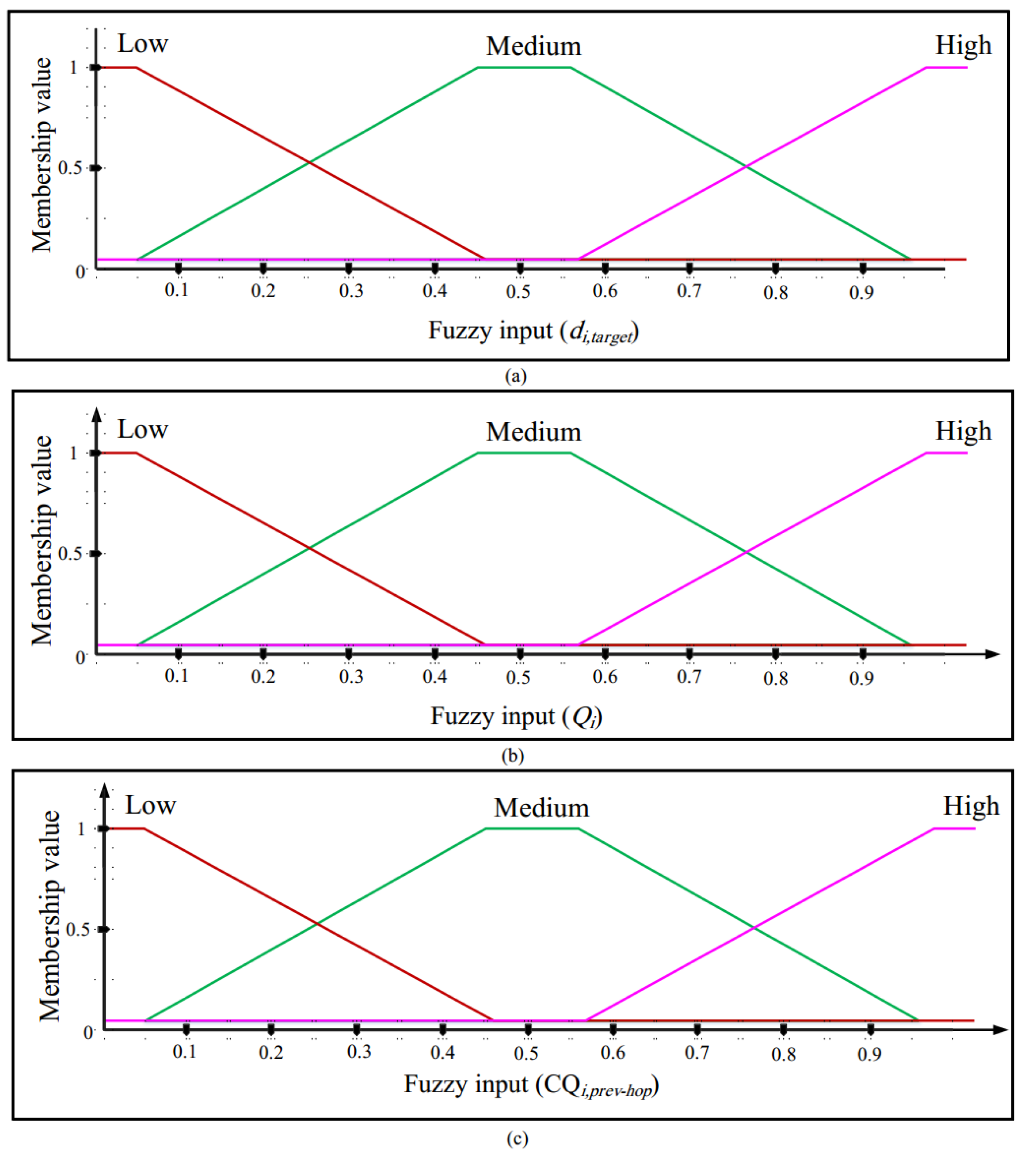
    where x i , y i and x t a r g e t , y t a r g e t display the spatial coordinates of V e h i c l e i and P T a r g e t , respectively. Moreover, L R indicates the length of the road related to V e h i c l e S . It is calculated using Equation (11). The membership function chart of d i , t a r g e t is presented in Figure 8a. It involves three states: low, medium, and high.
  • Queue status ( Q i ):  V e h i c l e S extracts Q i for each neighboring vehicle (such as V e h i c l e i ) from the neighbor table. The purpose of this parameter is to lower the chance of vehicles with high traffic being selected as the relay vehicle. See the membership function chart of Q i in Figure 8b. This input considers three states: low, medium, and high.
  • Connection Quality ( CQ i , prev hop ):  V e h i c l e S calculates C Q i , p r e v h o p for each neighboring node (such as V e h i c l e i ) using Equation (4) to be selected vehicle with the highest connection quality as the relay vehicle. The membership function chart of C Q i , p r e v h o p is represented in Figure 8c. This input involves three states: low, medium, and high.

Fuzzy Output

In the fuzzy route recovery process, the fuzzy output (i.e., S i ) determines the chances of neighboring vehicles being selected as the relay vehicle. In the proposed fuzzy system, a vehicle that has a short distance to P T a r g e t and includes low traffic, and a high connection quality compared to other neighboring vehicles, obtains a high chance to be selected as the relay vehicle. See the diagram of the fuzzy membership function related to S i in Figure 9. This fuzzy output consists of seven states: extremely low, very low, low, medium, high, very high, and extremely high.

Rule Base

Table 4 expresses the fuzzy rules introduced in the fuzzy route recovery algorithm. For example, ”Rule 1” is defined below:
Rule 1:  d i , t a r g e t is low AND  Q i is low AND  C Q i , p r e v h o p is Low THEN  S i is High.
Algorithm 3 V2V routing process
Input: 
V e h i c l e S : Source vehicle or intermediate node
  •          I n t e r s e c t S : Source intersection
  •          V e h i c l e D : Destination vehicle
Output: 
Next-hop node
  Begin
1:
if  V e h i c l e S and V e h i c l e D are on the same road section then
2:
    P T a r g e t = V e h i c l e D ;
3:
else if  V e h i c l e S is the source node then
4:
    P T a r g e t = I n t e r s e c t S ;
5:
else if  V e h i c l e S is the intermediate node then
6:
    P T a r g e t = I n t e r s e c t j t + 1 that is obtained using Algorithm 2;
7:
end if
8:
Vehicle S : Choose the nearest next-hop node to T a r g e t from its T a b l e n e i g h b o r ;
9:
if  V e h i c l e S cannot find the nearest next-hop node then
10:
    Vehicle S : Calculate S i for all neighbors based on d i , t a r g e t , Q i , C Q i , p r e v h o p using a fuzzy system;
11:
    Vehicle S : Choose the vehicle with maximum S i as the relay node;
12:
end if
13:
Vehicle S : Transmit the packet to the relay vehicle;
   End

5.3.3. Vehicle-to-Infrastructure (V2I) Routing Algorithm

In QFHR, when choosing the next-hop node in a road section, each vehicle uses a greedy routing technique for transferring packets to the intersection area. Then, RSU selects the next intersection by searching in Q-table calculated in the I2I routing algorithm described in Section 5.2. At this step, each RSU employs a greedy strategy to send packets to the related road section. In this case, there are two modes:
  • First mode:  V e h i c l e D moves in this road section. In this case, V e h i c l e D is determined as a target point ( P T a r g e t ).
  • Second mode:  V e h i c l e D does not move in this road section. In this case, the next intersection is considered as P T a r g e t .
Now, RSU checks its neighbor table to determine whether P T a r g e t is its neighbor or not. If P T a r g e t is in its neighbor table, the data packet is sent to P T a r g e t directly. Otherwise, RSU finds the vehicle closest to P T a r g e t in its neighbor table and transfers the packet to it. If RSU fails to find a vehicle to send the data packet, RSU stores this packet until it discovers the next-hop vehicle.
Algorithm 4 V2I routing process
Input: 
I n t e r s e c t i : Intermediate intersection
  •        I n t e r s e c t D : Destination intersection
  •        R S U i : RSU located in I n t e r s e c t i
  •        R S U D : RSU located in I n t e r s e c t D
  •        V e h i c l e D : Destination vehicle
Output: 
Next-hop node
 Begin
1:
if the intersection is I n t e r s e c t D  then
2:
    P T a r g e t = V e h i c l e D ;
3:
else if the intersection is I n t e r s e c t i
4:
    P T a r g e t = I n t e r s e c t j t + 1 that is obtained using Algorithm 2;
5:
end if
6:
if RSU is neighbor of P T a r g e t  then
7:
   RSU: Send the data packet to P T a r g e t directly;
8:
else
9:
   RSU: Find the closest relay node to P T a r g e t from its T a b l e n e i g h b o r ;
10:
   RSU: Send the packet to the relay node;
11:
end if
12:
if RSU cannot find the closest relay node to P T a r g e t  then
13:
   RSU: Carry the packet until it discovers an appropriate relay node;
14:
   while the buffer queue of RSU is not empty do
15:
     RSU: Check its T a b l e n e i g h b o r periodically;
16:
     if RSU finds a neighbor as the relay node then
17:
        RSU: Send the packet to the relay node;
18:
     end if
19:
   end while
20:
end if
   End

6. Simulates and Evaluation of Results

In this section, Network Simulator version 2 (NS2) [39] implements QFHR for evaluating its performance. When simulating QFHR, various parameters such as packet delivery rate, delay, hop count, and routing overhead are analyzed. Next, the results are compared with IRQ [29], IV2XQ [28], QGrid [27], and GPSR [26]. To achieve this goal, the dimensions of the network are 3 km × 3 km. It has 38 two-way road sections and 24 intersections. There are 5–20 vehicles in each kilometer. In the network, there are 450 vehicles whose speed is 14 m per second. It is assumed that the communication range of each vehicle varies between 250 and 300 m, and the communication range of each RSU is a fixed value (i.e., 300 m). The simulation time is considered 1000 s. Help messages are broadcast in a fixed time interval (1 s) and the packet sending rate is equal to 1–6 packets per second. Moreover, the packet size is 512 bytes. In QFHR, the Q-learning algorithm has a fixed learning rate ( α = 0.1 ) and uses an ϵ -greedy strategy in the exploration and exploitation processes, so that ϵ = 0.2 . Table 5 describes the simulation parameters.

6.1. Packet Delivery Rate (PDR)

Packet delivery rate (PDR) is defined as the ratio of packets received by the destination nodes to all packets transferred by the source nodes. In the simulation process, two scenarios are intended to evaluate the packet delivery rate. The purpose of the first scenario is to calculate PDR based on the packet sending rate (PSR). As shown in Figure 10, when PSR is high, PDR decreases in all methods and vice versa because the packet sending rate indicates the number of packets produced in the network per time unit. Therefore, high PSR increases the network load. In this case, the buffer capacity of vehicles is completed quickly, and it is very likely that some data packets will be lost due to high network congestion. Thus, PDR is reduced in the network. The purpose of the second scenario is to evaluate the packet delivery rate according to the signal transmission radius (STR) of vehicles. As shown in Figure 11, when STR is large, PDR will also increase because the number of single-hop neighbors of each vehicle increases in this case, and a vehicle can cover a wider communication range. In this case, vehicles have a higher chance to find a next-hop node. This reduces the probability of the local optimum issue. According to Figure 10 and Figure 11, QFHR has an optimal PDR in comparison with other approaches. In Figure 10, which shows the evaluation of PDR based on PSR, QFHR increases the packet delivery rate by 2.74%, 6.67%, 22.35%, and 29.98% compared to IRQ, IV2XQ, QGrid, and GPSR, respectively. Additionally, in Figure 11, which shows PDR based on STR, QFHR has improved PDR by 3.45%, 8%, 23.29%, and 26.17% compared to IRQ, IV2XQ, QGrid, and GPSR, respectively. This is mainly rooted in the fact that QFHR performs the Q-learning-based routing process using a distributed manner to discover various paths between network intersections. However, IRQ, IV2XQ, and QGrid present centralized routing processes. The distributed routing method is more compatible with the dynamic environment of VANET and can find routes with less delay and high connection quality in the network. Thus, it improves the packet delivery rate. Moreover, if the network has high congestion, QFHR can quickly discover this issue and replace the new path. However, IRQ selects the best route based on traffic information from the central server. In this scheme, the central server should wait for receiving traffic messages from RSUs to detect the congestion on the network. However, this process causes a high delay and may lose some data packets on the network. Furthermore, in IV2XQ, the central server chooses the best route based on historical traffic information stored in its memory, and the route selection process depends only on the vehicle density in the road sections. In addition, QGrid selects the best gird (i.e., the gird with maximum density) using a greedy routing process. However, the high-density grid is not always desirable and may cause congestion on the network and packet loss. GPSR is a greedy routing process and deals with the local minimum problem, which rises packet loss.

6.2. Delay

End-to-end delay is defined as the time required for sending packets from the source node to the destination node. The first scenario tests delay based on the packet sending rate. It is displayed in Figure 12. According to this figure, high PSR leads to high delay in all routing approaches because high PSR causes congestion in the network. As a result, data packets wait longer in the buffer queue, meaning that the queuing delay increases. Therefore, delay increases in the data transmission process. The second scenario evaluates delay based on the signal transmission radius (STR) of vehicles. This is shown in Figure 13. When STR is large, delay decreases in all methods because the number of hops is reduced in the routing path. According to Figure 12 and Figure 13, QFHR has the least delay compared to other approaches. In Figure 12, the proposed scheme lowers delay by 16.19%, 22.82%, 34.15%, and 59.51%, compared to IRQ, IV2XQ, QGrid, and GPSR, respectively. Moreover, in Figure 13, QFHR decreases delay by 19.86%, 34.26%, 44.09%, and 68.39% compared to IRQ, IV2XQ, QGrid, and GPSR, respectively, because QFHR uses a distributed Q-learning-based routing process to choose the next intersection with regard to road congestion status and road connection quality. In addition, in the V2V routing process at each road section, a fuzzy logic-based route recovery process is considered to obtain the next-hop vehicle in accordance to the queue status and the connection quality of vehicles. These techniques can prevent congestion in the network and lower delay in the operation. On the other hand, IRQ, IV2XQ, and QGrid are centralized routing methods because the central server performs the route discovery process and sends it to vehicles on the network. This boosts the delay in the packet transmission operation. Moreover, IRQ must periodically send traffic messages to the central server to calculate routes based on these messages. This is another factor in increasing delay in IRQ. Note that IRQ and IV2XQ are equipped with a congestion control mechanism. Thus, they have an acceptable delay. However, QGrid has not designed any congestion control mechanism on the network. This is the most important reason for the high delay in this method. GPSR has also experienced the worst delay in comparison with other methods because it involves the local optimum problem.

6.3. Hop Count

Hop count is defined as the average number of intermediate nodes in the routing path between the source node and the destination node. The first scenario evaluates the number of hops based on the packet-sending rate. It is represented in Figure 14. Based on this figure, we can deduce that the number of hops has a direct relationship with the packet sending rate (PSR), meaning that high PSR leads to a high number of hops in the routing path because high PSR causes congestion in the network and has a negative impact on the routing process. QFHR has lowered the number of hops compared to IRQ, IV2XQ, QGrid, and GPSR, by 6.74%, 20.09%, 2.68%, and 12.22%, respectively. The second scenario evaluates the number of hops based on the signal transmission radius (STR). It is represented in Figure 15. According to this figure, when STR has a large value, the number of intermediate nodes in the path decreases. QFHR lowers the number of hops by 14.13%, 32.58%, 7.71%, and 21.39% compared to IRQ, IV2XQ, QGrid, and GPSR, respectively.

6.4. Routing Overhead

Routing overhead is equal to the ratio of the total failed data packets in the data transfer process and control packets in the route discovery and maintenance processes to all the packets produced in the network. The first scenario tests the routing overhead based on the packet sending rate. It is displayed in Figure 16. According to this figure, there is a direct relationship between PSR and routing overhead, meaning that when the packet sending rate goes up, the routing overhead increases because high PSR increases the collision probability and the packet loss due to network congestion. As a result, the need for retransferring packets increases, and it increases routing overhead. The second scenario has evaluated the overhead in various methods based on the signal transmission radius (STR), and its results are shown in Figure 17. This figure shows that high STR leads to low overhead because the packet delivery rate is high, which reduces the need for retransferring data packets. According to Figure 16, which evaluates the overhead based on PSR, QFHR reduces the overhead by 30.23% and 41.4% compared to QGrid and GPSR, respectively. However, the proposed method increases the overhead by approximately 9.36% and 11.34% compared to IRQ and IV2XQ, respectively. Moreover, according to Figure 17, which shows the overhead based on the signal transmission radius, QFHR decreases overhead by 21.99% and 25.63% compared to QGrid and GPSR, respectively. However, it has a higher overhead than IRQ (11.26%) and IV2XQ (25%). IV2XQ uses historical traffic information stored in the server memory in the Q-learning-based routing process to discover paths between network intersections, meaning that it does not exchange any control packet for discovering these routes. As a result, the overhead is extremely low in this method. Whereas, in QFHR, RSUs are responsible for discovering routes between intersections, and traffic information is periodically updated. This has increased routing overhead in this scheme. GPSR has the worst routing overhead due to the local optimum problem. QGrid also has high routing overhead because it has not used any congestion mechanism. As a result, when increasing congestion in the network, packet loss increases. This increases the need for retransferring data packets.

7. Conclusions

In this paper, a Q-learning and fuzzy logic-based hierarchical routing approach (QFHR) was suggested for VANETs. In the first step, a traffic identification algorithm was presented so that each RSU obtains information about the traffic conditions of four roads connected to its intersection. Next, each RSU uses this traffic information to design the Q-learning-based routing algorithm to discover the most suitable path between different intersections. In the last step, the routing algorithm at the road level was introduced. It is a greedy routing algorithm that uses fuzzy logic to recover routes and solve the local optimum problem. QFHR was implemented using NS2. Then, the results were compared with IRQ, IV2XQ, QGrid, and GPSR in two scenarios. The first scenario analyzes the result based on the packet sending rate (PSR). In this scenario, QFHR increases PDR by 2.74%, 6.67%, 22.35%, and 29.98% and reduces delay by 16.19%, 22.82%, 34.15%, and 59.51%, and lowers the number of hops by 6.74%, 20.09%, 2.68%, and 12.22% compared with IRQ, IV2XQ, QGrid, and GPSR, respectively. However, it increases the overhead by approximately 9.36% and 11.34% compared to IRQ and IV2XQ, respectively. Additionally, the second scenario evaluates the results with regard to the signal transmission radius (STR). In this scenario, QFHR increases PDR by 3.45%, 8%, 23.29%, and 26.17% and decreases delay by 19.86%, 34.26%, 44.09%, and 68.39% and reduces the number of hops by 14.13%, 32.58%, 7.71%, and 21.39% compared to IRQ, IV2XQ, QGrid, and GPSR, respectively. However, it has a higher overhead than IRQ (11.26%) and IV2XQ (25%). These results show that QFHR has a good performance in terms of PDR, delay, and the number of hops. However, the proposed method has a greater routing overhead than IRQ and IV2XQ. In future research directions, our focus is on reducing the routing overhead in QFHR. This can be achieved in two schemes: (1) Providing a clustering technique to increase scalability and reduce routing overhead and (2) adjusting the hello broadcast interval dynamically in accordance with road traffic conditions.

Author Contributions

Conceptualization, M.S.Y., E.Y.; methodology, M.S.Y., E.Y., M.H.; validation, A.M.R., R.A.N., O.H.A.; investigation, A.M.R., R.A.N., K.S.; resources, A.M.R., O.H.A.; writing—original draft preparation, M.S.Y., E.Y., K.S.; supervision, M.H.; project administration, M.H., K.S. All authors have read and agreed to the published version of the manuscript.

Funding

This research was supported by Xiamen University Malaysia Research Fund (Grant Number: XMUMRF/2022-C9/IECE/0033).

Data Availability Statement

Not applicable.

Conflicts of Interest

The authors declare no conflict of interest.

References

  1. Mchergui, A.; Moulahi, T.; Zeadally, S. Survey on Artificial Intelligence (AI) Techniques for Vehicular ad-hoc Networks (VANETs). Veh. Commun. 2021, 100403. [Google Scholar] [CrossRef]
  2. Xia, Z.; Wu, J.; Wu, L.; Chen, Y.; Yang, J.; Yu, P.S. A comprehensive survey of the key technologies and challenges surrounding vehicular ad hoc networks. ACM Trans. Intell. Syst. Technol. (TIST) 2021, 12, 1–30. [Google Scholar] [CrossRef]
  3. Abdelgadir, M.; Saeed, R.A.; Babiker, A. Mobility Routing Model for Vehicular ad-hoc Networks (VANETs), Smart City Scenarios. Veh. Commun. 2017, 9, 154–161. [Google Scholar] [CrossRef]
  4. Li, H.; Liu, Y.; Qin, Z.; Rong, H.; Liu, Q. A large-scale urban vehicular network framework for IoT in smart cities. IEEE Access 2019, 7, 74437–74449. [Google Scholar] [CrossRef]
  5. Mustakim, H.U. 5G vehicular network for smart vehicles in smart city: A review. J. Comput. Electron. Telecommun. 2020, 1. [Google Scholar] [CrossRef]
  6. Quy, V.K.; Nam, V.H.; Linh, D.M.; Ban, N.T.; Han, N.D. Communication Solutions for Vehicle ad-hoc Network in Smart Cities Environment: A Comprehensive Survey. Wirel. Pers. Commun. 2021, 122, 2791–2815. [Google Scholar] [CrossRef]
  7. Li, F.; Wang, Y. Routing in vehicular ad hoc networks: A survey. IEEE Veh. Technol. Mag. 2007, 2, 12–22. [Google Scholar] [CrossRef]
  8. Domingos, F.; Villas, L.; Boukerche, A. Data Communication in VANETs: Survey, Applications and Challenges. Ad Hoc Netw. 2016, 44, 90–103. [Google Scholar]
  9. Lee, S.W.; Ali, S.; Yousefpoor, M.S.; Yousefpoor, E.; Lalbakhsh, P.; Javaheri, D.; Rahmani, A.M.; Hosseinzadeh, M. An energy-aware and predictive fuzzy logic-based routing scheme in flying ad hoc networks (fanets). IEEE Access 2021, 9, 129977–130005. [Google Scholar] [CrossRef]
  10. Rahmani, A.M.; Ali, S.; Yousefpoor, M.S.; Yousefpoor, E.; Naqvi, R.A.; Siddique, K.; Hosseinzadeh, M. An area coverage scheme based on fuzzy logic and shuffled frog-leaping algorithm (sfla) in heterogeneous wireless sensor networks. Mathematics 2021, 9, 2251. [Google Scholar] [CrossRef]
  11. Dua, A.; Kumar, N.; Bawa, S. A Systematic Review on Routing Protocols for Vehicular ad hoc Networks. Veh. Commun. 2014, 1, 33–52. [Google Scholar] [CrossRef]
  12. Boussoufa-Lahlah, S.; Semchedine, F.; Bouallouche-Medjkoune, L. Geographic routing protocols for Vehicular Ad hoc NETworks (VANETs): A survey. Veh. Commun. 2018, 11, 20–31. [Google Scholar] [CrossRef]
  13. Aggarwal, A.; Gaba, S.; Nagpal, S.; Vig, B. Bio-Inspired Routing in VANET. Cloud IoT-Based Veh. Ad Hoc Netw. 2021, 199–220. [Google Scholar] [CrossRef]
  14. Ksouri, C.; Jemili, I.; Mosbah, M.; Belghith, A. Towards general Internet of Vehicles networking: Routing protocols survey. Concurr. Comput. Pract. Exp. 2022, 34, e5994. [Google Scholar] [CrossRef]
  15. Teixeira, L.H.; Huszák, Á. Reinforcement Learning Environment for Advanced Vehicular Ad Hoc Networks Communication Systems. Sensors 2022, 22, 4732. [Google Scholar] [CrossRef] [PubMed]
  16. Pateria, S.; Subagdja, B.; Tan, A.H.; Quek, C. Hierarchical reinforcement learning: A comprehensive survey. ACM Comput. Surv. (CSUR) 2021, 54, 1–35. [Google Scholar] [CrossRef]
  17. Genders, W.; Razavi, S. Asynchronous n-step Q-learning adaptive traffic signal control. J. Intell. Transp. Syst. 2019, 23, 319–331. [Google Scholar] [CrossRef]
  18. Chen, X.; Wu, S.; Shi, C.; Huang, Y.; Yang, Y.; Ke, R.; Zhao, J. Sensing data supported traffic flow prediction via denoising schemes and ANN: A comparison. IEEE Sens. J. 2020, 20, 14317–14328. [Google Scholar] [CrossRef]
  19. Gronauer, S.; Diepold, K. Multi-agent deep reinforcement learning: A survey. Artif. Intell. Rev. 2022, 55, 895–943. [Google Scholar] [CrossRef]
  20. Chen, W.; Qiu, X.; Cai, T.; Dai, H.N.; Zheng, Z.; Zhang, Y. Deep reinforcement learning for Internet of Things: A comprehensive survey. IEEE Commun. Surv. Tutor. 2021, 23, 1659–1692. [Google Scholar] [CrossRef]
  21. Sun, Y.; Lin, Y.; Tang, Y. A reinforcement learning-based routing protocol in VANETs. In International Conference in Communications, Signal Processing, and Systems; Springer: Singapore, 2017; pp. 2493–2500. [Google Scholar] [CrossRef]
  22. Roh, B.S.; Han, M.H.; Ham, J.H.; Kim, K.I. Q-LBR: Q-learning based load balancing routing for UAV-assisted VANET. Sensors 2020, 20, 5685. [Google Scholar] [CrossRef] [PubMed]
  23. Bi, X.; Gao, D.; Yang, M. A reinforcement learning-based routing protocol for clustered EV-VANET. In Proceedings of the 2020 IEEE 5th Information Technology and Mechatronics Engineering Conference (ITOEC), Chongqing, China, 12–14 June 2020; pp. 1769–1773. [Google Scholar] [CrossRef]
  24. Yang, X.; Zhang, W.; Lu, H.; Zhao, L. V2V routing in VANET based on heuristic Q-learning. Int. J. Comput. Commun. Control 2020, 15. [Google Scholar] [CrossRef]
  25. Wu, C.; Yoshinaga, T.; Bayar, D.; Ji, Y. Learning for adaptive anycast in vehicular delay tolerant networks. J. Ambient Intell. Humaniz. Comput. 2019, 10, 1379–1388. [Google Scholar] [CrossRef]
  26. Karp, B.; Kung, H.T. GPSR: Greedy perimeter stateless routing for wireless networks. In Proceedings of the 6th Annual International Conference on Mobile Computing and Networking, Boston, MA, USA, 6–11 August 2000; pp. 243–254. [Google Scholar]
  27. Li, F.; Song, X.; Chen, H.; Li, X.; Wang, Y. Hierarchical routing for vehicular ad hoc networks via reinforcement learning. IEEE Trans. Veh. Technol. 2018, 68, 1852–1865. [Google Scholar] [CrossRef]
  28. Luo, L.; Sheng, L.; Yu, H.; Sun, G. Intersection-based V2X routing via reinforcement learning in vehicular Ad Hoc networks. IEEE Trans. Intell. Transp. Syst. 2021, 23, 5446–5459. [Google Scholar] [CrossRef]
  29. Khan, M.U.; Hosseinzadeh, M.; Mosavi, A. An Intersection-Based Routing Scheme Using Q-Learning in Vehicular Ad Hoc Networks for Traffic Management in the Intelligent Transportation System. Mathematics 2022, 10, 3731. [Google Scholar] [CrossRef]
  30. Rezwan, S.; Choi, W. A survey on applications of reinforcement learning in flying ad-hoc networks. Electronics 2021, 10, 449. [Google Scholar] [CrossRef]
  31. Padakandla, S. A survey of reinforcement learning algorithms for dynamically varying environments. ACM Comput. Surv. (CSUR) 2021, 54, 1–25. [Google Scholar] [CrossRef]
  32. Al-Rawi, H.A.; Ng, M.A.; Yau, K.L.A. Application of reinforcement learning to routing in distributed wireless networks: A review. Artif. Intell. Review. 2015, 43, 381–416. [Google Scholar] [CrossRef]
  33. Rahmani, A.M.; Yousefpoor, E.; Yousefpoor, M.S.; Mehmood, Z.; Haider, A.; Hosseinzadeh, M.; Ali Naqvi, R. Machine learning (ML) in medicine: Review, applications, and challenges. Mathematics 2021, 9, 2970. [Google Scholar] [CrossRef]
  34. Dumitrescu, C.; Ciotirnae, P.; Vizitiu, C. Fuzzy logic for intelligent control system using soft computing applications. Sensors 2021, 21, 2617. [Google Scholar] [CrossRef] [PubMed]
  35. Nadaban, S. From classical logic to fuzzy logic and quantum logic: A general view. Int. J. Comput. Commun. Control 2021, 16. [Google Scholar] [CrossRef]
  36. van Krieken, E.; Acar, E.; van Harmelen, F. Analyzing differentiable fuzzy logic operators. Artif. Intell. 2022, 302, 103602. [Google Scholar] [CrossRef]
  37. Perry, M.B. The exponentially weighted moving average. Wiley Encycl. Oper. Res. Manag. Sci. 2010. [Google Scholar] [CrossRef]
  38. Nabi, M.; Geilen, M.M.; Basten, T.A. An empirical study of link quality estimation techniques for disconnection detection in WBANs. In Proceedings of the 16th ACM International Conference on Modeling, Analysis & Simulation of Wireless and Mobile Systems, Barcelona, Spain, 3–8 November 2013; pp. 219–228. [Google Scholar]
  39. Altman, E.; Jimenez, T. NS Simulator for beginners. Synth. Lect. Commun. Netw. 2012, 5, 1–184. [Google Scholar]
Figure 1. Intelligent transportation system (ITS) in smart city.
Mathematics 10 04192 g001
Figure 2. Reinforcement learning process.
Mathematics 10 04192 g002
Figure 3. Network model in QFHR.
Mathematics 10 04192 g003
Figure 4. Hello message broadcast.
Mathematics 10 04192 g004
Figure 5. The movement of vehicles in the same direction (a) V e h i c l e i is ahead of V e h i c l e j . (b) V e h i c l e i is behind V e h i c l e j .
Mathematics 10 04192 g005
Figure 6. The movement of vehicles in the opposite direction (a) V e h i c l e i approaches V e h i c l e j . (b) V e h i c l e i gets away from V e h i c l e j .
Mathematics 10 04192 g006
Figure 7. Different components in I2I routing model in QFHR.
Mathematics 10 04192 g007
Figure 8. Fuzzy inputs.
Mathematics 10 04192 g008
Figure 9. Fuzzy output.
Mathematics 10 04192 g009
Figure 10. PDR in different approaches based on PSR.
Mathematics 10 04192 g010
Figure 11. PDR in different approaches based on STR.
Mathematics 10 04192 g011
Figure 12. Average delay in different approaches according to PSR.
Mathematics 10 04192 g012
Figure 13. Average delay in different routing approaches according to STR.
Mathematics 10 04192 g013
Figure 14. Average number of hops in different approaches with regard to PSR.
Mathematics 10 04192 g014
Figure 15. Average number of hops in different approaches with regard to STR.
Mathematics 10 04192 g015
Figure 16. Routing overhead in different approaches based on PSR.
Mathematics 10 04192 g016
Figure 17. Routing overhead in different approaches based on STR.
Mathematics 10 04192 g017
Table 1. The strengths and weaknesses of the related works.
MethodStrengthsWeaknesses
PbQR [21]Stability of communication links, improving packet transmission rate, reducing delay in the routing process, high scalabilityApplying a greedy approach to obtain Q-value from Q-table, high dependence on RSU, not considering traffic lights as warning signs
Q-LBR [22]Low routing overhead, high packet transmission rate, stability of communication links, suitable for urban areas during natural disasters, high scalabilityNot considering a mechanism for adding drones to the network, not providing techniques to calculate the optimal height of drones, not specifying the number of drones
RLRC [23]Considering the optimal energy consumption in electric vehicles, using SARSA for optimizing the routing process, scalabilityHigh bandwidth consumption, high delay, low throughput, not paying attention to motion direction
HQVR [24]Determining the learning rate based on the link quality, increasing packet delivery rate, reducing the effect of the node mobility on the convergence speed of Q-learning algorithm, low dependence on infrastructure (RSUs)High dependence of Q-learning algorithm to beacon messages, slow convergence speed of the learning algorithm, applying an exploration technique based on a specific probability
QVDRP [25]High delay-tolerant, increasing packet delivery rate, reducing the number of duplicated control messages, considering relative velocity of vehiclesSlow convergence speed of the learning algorithm
GPSR [26]Reducing routing overhead, reducing delay in the networkNot considering factors, like velocity, movement direction, and link lifetime in the routing process
QGrid [27]Reducing the number of states in Q-learning algorithm, appropriate convergence speed, reducing communication overhead, determining the discount factor based on vehicle densityDesigning an off-line routing, not designing a congestion control mechanism in the network, fixing Q-table during the simulation process, not considering the effect of intersections and buildings on the transmission quality in each grid, not considering parameters such as speed, movement direction, and link lifetime in the routing process, introducing a centralized reinforcement learning-based routing algorithm
IV2XQ [28]Determining the discount factor with regard to the density and distance of vehicles on the road section, reducing communication overhead, designing a congestion control mechanism, appropriate convergence speed, reducing the number of states in the Q-learning algorithmNot considering factors, like speed, movement direction, and link lifetime in the routing process, not relying on new traffic information in the network, introducing a centralized reinforcement learning-based routing algorithm
IRQ [29]Adjusting the discount factor with regard to the vehicle density and distance, high PDR, reducing latency in the routing process, presenting a evaluation mechanism for controlling the congested paths, suitable convergence speed, reducing the number of states in the Q-learning algorithm, considering new traffic information in the networkHigh routing overhead, introducing a centralized reinforcement learning-based routing algorithm
Table 2. Neighbor table format.
Vehicle IDRoad IDSpatial CoordinatesSpeedQueue StatusConnection Quality   Validity Time
I D j I D R x j , y j v x , j , v y , j Q j C Q i , j V T j
Table 3. Traffic table format.
Road IDRoad LengthAverage Road TimeVehicle DensityCongestion StatusAverage Connection QualityValidity Time
R N o r t h Northern road lengthAverage northern road timeThe number of vehicles in the northern roadAverage congestion status in the northern roadAverage connection quality in the northern road V T R N o r t h
R S o u t h Southern road lengthAverage southern road timeThe number of vehicles in the southern roadAverage congestion status in the southern roadAverage connection quality in the southern road V T R S o u t h
R E a s t Eastern road lengthAverage eastern road timeThe number of vehicles in the eastern roadAverage congestion status in the eastern roadAverage connection quality in the eastern road V T R E a s t
R W e s t Western road lengthAverage western road timeThe number of vehicles in the western roadAverage congestion status in the western roadAverage connection quality in the western road V T R W e s t
Table 4. Fuzzy rule base in proposed fuzzy system.
Fuzzy System InputsFuzzy System Output
Fuzzy Rules d i , target Q i CQ i , prev hop S i
1LowLowLowHigh
2LowLowMediumVery high
3LowLowHighExtermely high
4LowMediumLowMedium
5LowMediumMediumHigh
6LowMediumHighVery high
7LowHighLowLow
8LowHighMediumMedium
9LowHighHighHigh
10MediumLowLowMedium
11MediumLowMediumHigh
12MediumLowHighVery high
13MediumMediumLowLow
14MediumMediumMediumMedium
15MediumMediumHighHigh
16MediumHighLowVery low
17MediumHighMediumLow
18MediumHighHighMedium
19HighLowLowLow
20HighLowMediumMedium
21HighLowHighHigh
22HighMediumLowVery low
23HighMediumMediumLow
24HighMediumHighMedium
25HighHighLowExtermely low
26HighHighMediumVery low
27HighHighHighLow
Table 5. Simulation parameters.
ParametersValue
Network simulatorNS2
Network size 3 × 3 km2
Simulation time1000 s
Vehicles450
Road sections38
Intersections24
Vehicle density0.005–0.02 (Vehicle/m)
Vehicle velocity14  m/s
Communication range of vehicles250–300 m
Communication range of RSUs300 m
Packet size512 byte
Packet sending rate1–6 (Packet/s)
Hello broadcast period1 s
Learning rate ( α )0.1
ϵ 0.2
Publisher’s Note: MDPI stays neutral with regard to jurisdictional claims in published maps and institutional affiliations.