Earthquake Catastrophe Bond Pricing Using Extreme Value Theory: A Mini-Review Approach

Abstract

Earthquake catastrophe bond pricing models (ECBPMs) employ extreme value theory (EVT) to predict severe losses, although studies on EVT’s use in ECBPMs are still rare. Therefore, this study aimed to use a mini-review approach (MRA) to examine the use of EVT and identify the gaps and weaknesses in the methods or models developed. The MRA stages include planning, search and selection, analysis, and interpretation of the results. The selection results showed five articles regarding the application of EVT in ECBPMs. Furthermore, the analysis found the following: First, the generalized extreme value (GEV) could eliminate extreme data in a period. Second, the trigger model using two parameters is better than one, but the study did not discuss the joint distribution of the two parameters. Third, the autoregressive integrated moving average (ARIMA) allows negative values. Fourth, Cox–Ingersoll–Ross (CIR) in-coupon modeling is less effective in depicting the real picture. This is because it has a constant volatility assumption and cannot describe jumps due to monetary policy. Based on these limitations, it is hoped that future studies can develop an ECBPM that reduces the moral hazard.

1. Introduction

Large-magnitude earthquakes cause extensive damage, loss of life, and economic losses in developing and developed countries [1,2,3,4,5]. Examples include the earthquakes in Colombia (1999, 6.2 Mw, 2000 victims) [6], Haiti (Hispaniola, 2010, 7.0 Mw, 222.570 victims, USD 8 billion in economic losses), Indonesia (Aceh, 2004, 165,708 victims, USD 4.4 billion), Iran (2003, 26,976 victims, USD 0.5 billion), Pakistan (2005, 73,338 victims, USD 5.2 billion) [7], Mexico (Gulf of Tehuantepec, 8.2 Mw, 2017, 98 victims) [8], Peru (45 km west-northwest of Chincha Alta, 2007, 8.0 Mw, 519 victims) [9], China (Wenchuan, 2008, 87,476 victims, USD 85 billion) [7], Chile (2010, 8.8 Mw, 521 victims, USD 30 billion) [10], Tohoku (2012, 9 Mw, 15,000 victims, USD 411 billion), and Nepal (2015, 7.8 Mw, 8000 victims) [11]. The potential for economic losses due to earthquakes keeps increasing due to the development of the socioeconomic system and urbanization [12]. The disaster management funds are insufficient to cover the losses suffered [13]. Therefore, there is a need for an alternative funding mechanism linked to the financial market, such as catastrophe bonds [14].

The countries that have sponsored earthquake bonds and collaborated with the World Bank in their issuance are Mexico, Peru, Chile, Colombia, and the Philippines.

Table 1. Earthquake catastrophe bonds issued by the World Bank.

Date of Issues	Sponsor	SPV	Value	Peril	Trigger Type
May 2006	FONDEN	Cat-Mex Ltd.	USD 160 million	Earthquake in Mexico	Parametric
October 2009	FONDEN	Multicat Mexico Ltd.	USD 290 million	Tornado and earthquake in Mexico	Parametric
August 2017	FONDEN	IBRBD CAR 113–115	The US $360 Million	Tornado and earthquake in Mexico	Parametric
February 2018	Republic of Chile	IBRD CAR 116	USD 500 million	Earthquake in Chile	Parametric
February 2018	Republic of Colombia	IBRD CAR 117	USD 400 million	Earthquake in Colombia	Parametric
February 2018	FONDEN	IRBD CAR 118–119	USD 260 million	Earthquake in Mexico	Parametric
February 2018	Republic of Peru	IBRD CAR 120	USD 200 million	Earthquake in Peru	Parametric
November 2019	Republic of the Philippines	World Bank IBRD 123–124	USD 225 million	Earthquake and tropical cyclone in the Philippines	Modeled loss

Source: www.artemis.bm, accessed on 5 May 2022, note: SPV (Special Purpose Vehicle).

presents the data related to the issuance.

The data in Table 1 show that the World Bank’s earthquake catastrophe bonds range from USD 160 million to USD 500 million. On 8 September 2017, Mexico was rocked by an earthquake of magnitude 8 Mw, causing investors to lose all cash and coupon values. Similarly, the 2018 earthquake in Peru, with a magnitude of 8 Mw, caused investors to lose 30% of their cash value. Based on this real case, earthquake bonds aid the sponsoring countries in procuring disaster funds. However, they pose a moral hazard to investors [13,14,15] due to disaster losses that must be borne by sponsors approaching the trigger specified in eliminating the law pliers. When this happens, no investors will be drawn to purchase the bonds. Therefore, an accurate and transparent earthquake catastrophe bond pricing model is required in order to succeed in the market [16].

In earthquake bond pricing, the catastrophe risk needs to be modeled first. Extreme events related to historical observations can be described using EVT. In particular, the theory of extreme values in catastrophe bonds (CAT bonds) is used to study the distribution of extreme values related to the trigger parameters used in the model (e.g., loss, mortality, flood height, earthquake magnitude, etc.).

The systematic reviews of CAT bonds that have been carried out previously are briefly described in this paragraph. Pizzutilo and Venezia [17] analyzed the effectiveness of catastrophe bonds for the transportation and infrastructure industries; the results showed that catastrophe bonds benefit from managing potential losses related to disaster events. Calvet et al. [18] reviewed statistical and machine learning methods in designing trigger mechanisms; the results indicated that statistical methods and machine learning provide great gains in accuracy and efficiency by decreasing the classification time. Wu and Zhou [19] reviewed the catastrophe bond instrument and the modeling approach used; the study found that the three most popular models used in modeling disaster losses are the compound Poisson model, jump diffusion, and double-exponential jump diffusion. Sukono et al. [20] also reviewed the use of the compound Poisson process; the results were obtained for 30 selected articles, with 12 articles using constant interest rates, while 18 did not; furthermore, 8 articles used CIR, 5 articles used Vasicek, 2 used the robust approach, 1 article used CIR and Vasicek, 1 used the Hull–White model, and 1 article used the ARIMA method.

The published literature review articles have not discussed the use of EVT. Therefore, this study aimed to use a mini-review approach (MRA) to examine the use of EVT on earthquake bonds and determine the literature gaps and limitations of the methods or models developed in the ECBPM. The study’s novelty is as follows:

(a)

Discussing the implementation of EVT in an ECBPM;

(b)

Analyzing the methods or models used in developing the ECBPM;

(c)

Discussing the literature gaps of the selected articles;

(d)

Performing bibliometric analysis based on co-words.

The MRA stages in this study consisted of planning, searching, analyzing, and interpreting the results. The study questions were prepared in the planning stage. The searching stage involved choosing the digital libraries, including Scopus, ScienceDirect, and ProQuest; this stage also involved defining, executing, and improving the keywords, as well as selecting the initial articles. The selection process used the Preferred Reporting Items for Systematic Reviews and Meta-Analyses (PRISMA) based on inclusion and exclusion criteria. The analysis stage examined the mathematical model, compared its achievements, and discussed the literature gap by analyzing the model’s limitations based on the assumptions of each method. This stage also provided alternative models to improve the limitations of the previous model through theoretical studies. Co-word bibliometric analysis was performed using the VOSviewer application. The results were expected to provide knowledge about the application of EVT. Additionally, they could suggest alternative models for use in developing ECBPMs. The findings could also motivate future studies on the development of ECBPMs.

2. Introductory Literature on the Study Topic

Hurricane Andrew sent 11 insurance firms into bankruptcy because they lacked sufficient reserves to meet claims. As a result, catastrophe bonds were developed in the middle of 1990 [21]. The Chicago Board of Trade launched the first contract in 1992 and introduced a trigger put-and-call option for catastrophes. This option was based on the Catastrophe Loss Index compiled by the Property Claims Service (PCS) and the industry’s statistics agency [22]. Over time, CAT bonds are used by reinsurance companies and countries with a high potential for losses due to disasters to obtain alternative funding for disaster management.

Earthquake catastrophe bond pricing models (ECBPMs) require a detailed study of extreme losses, and the disaster severity is analyzed using EVT [23,24]. The extreme value theory of catastrophe bonds was used by Riza et al. [25] to model the distribution of actual losses and fatalities. Using multiple triggers, the study designed a price model for determining disaster bonds with and without coupons. ARIMA was used to model interest and coupon rates, while Burr, GEV, Weibull, GPD, and logistical models were employed to model the distribution of losses and deaths. Furthermore, maximum likelihood estimation (MLE) was used to estimate the parameters, while the nonhomogeneous Poisson process (NHPP) was used to determine the aggregate loss and death. The Nuel recursive method was used to calculate the CDF value of the NHPP. The simulation used data on storm catastrophe losses and fatalities in the United States from 2012 to 2021, the number of storms that occurred in the United States from 1986 to 2021, and USD LIBOR data from 1986 to 2021. The results of the analysis showed that the intensity of the disaster and factors such as the threshold value of losses and deaths affect the price of catastrophe bonds. More intense disasters and longer bond periods reduce the bond price. Additionally, a greater threshold value of the two triggers increases the bond price.

Marvi et al. [26] modeled multi-period bond pricing for multi-hazard and multiregional disasters. The study used GEV type II or Frechet methods to model the distribution of water levels and employed a binary function to model cash value. The Monte Carlo simulation method was used to generate water level data, and a hydraulic flow model was used to determine the flood depth and flood intensity in buildings in an area. The multi-hazard and multiregional models could reduce the residual risk and benefit the insurance companies.

Chao [27] developed a methodology to account for various risks while pricing multi-period catastrophe bonds. The Poisson process was used to model the number of disaster events up to time t, while the CIR and GPD were used to model interest rates and the distribution of loss variables, respectively. Furthermore, the MLE was used to estimate the parameters, while the copula was used to model the dependence distribution of economic losses and deaths. The Kolmogorov–Smirnov test was used to assess the viability of choosing the copula model, and the sensitivity analysis was used to evaluate the impact of interest rates and GPD parameters on the bonds. The findings showed that the interest and the average long-term interest rates have an inverse relationship with catastrophe bond prices. However, there was a strong correlation between economic losses and mortality raising the price of disaster bonds.

Deng et al. [28] modeled multi-period drought bond prices. POT was used to determine the loss threshold, while GPD was employed to model the distribution of losses. Moreover, the study used a binary function to model the face value of bonds and a Poisson process to determine the number of disasters at time t. The Lagrange method, also known as MLE, was used to estimate the GPD distribution parameters. The results showed that a higher probability of a disaster-triggering event reduces catastrophe bond prices. High-risk investments provide a high-yield stimulus and attract many investors.

Chao and Zhou [29] modeled multi-period catastrophe bond pricing. The study used the Poisson process to determine the number of disaster bonds at time t and the CIR to model the interest rate. POT was used to obtain extreme values of deaths and economic losses due to disasters. Moreover, the copula was used to model the dependency distribution of deaths and economic losses, while Monte Carlo simulations were utilized for the experiments. The sensitivity analysis determined the impact of disaster intensity, maturity time, and the magnitude of the tau–Kendall correlation on catastrophe bond prices. The results showed that a catastrophe bond pricing model triggered by many events has a lower risk than a model with a single triggering event. It also has a larger market potential than ordinary bonds and has low risk and high returns, reducing the moral hazard. Catastrophe bond prices have an inverse relationship with disaster intensity, maturity time, and the value of the tau–Kendall correlation. The disaster intensity’s effect on the maturity time is greater than that on the price.

The previously developed model was applied to storms [25], floods, and drought [28], and is generally not specific to drought, earthquakes, or floods [29]. The trigger types used were modeled loss [25,27,28], industry loss [29], and parametric [26]. The parametric trigger type has high transparency and baseline risk, short settlement time, and low regulatory acceptance, while the opposite is true for the indemnity type [30]. This shows that the parametric type is better than other triggers for investors but poses a basic risk to the sponsor. In comparison, the GEV distribution could eliminate other extreme data in a period [27]. Investors also face financial risk, implying fluctuating interest rates, inflation, and coupons that affect the cash value of bonds. The model’s methods are ARIMA [25] and CIR [15,21]. However, ARIMA allows negative values. CIR also assumes constant volatility, which is unrealistic.

3. Materials and Methods

3.1. Materials

The first study materials were articles discussing mathematical modeling for determining the price of earthquake bonds using EVT, published in Scopus-indexed journals. The articles used were obtained from Scopus, ScienceDirect, and ProQuest, published between 2000 and 2022. The selected articles were mapped using bibliometric co-word analysis with the help of the VOSviewer application. Earthquake bonds were selected due to the increased potential for losses caused by earthquakes. The extreme value theory describes extreme losses due to disasters [31]. Scopus and ScienceDirect were chosen because they are reliable and popular search engine databases [25,32], while ProQuest has a science database, a strong collection of scientific journals, and more complete texts. The second study materials were the mathematical models employed in the modeling.

3.2. Methods

This research is a preliminary scientific exploration of using EVT in the evaluation of earthquake bonds. The research method consisted of tracing primary literature studies using MRA to remind us of the limited scope. This approach was used to identify literature gaps and limitations of the methods or models developed, as well as to obtain state-of-the-art help in developing a model for determining the price of bonds for earthquake disasters in the future. The aim of a thorough systematic study is to review all of the reliable data. To control the volume of material with limited resources, the extent of the search may be subject to arbitrary constraints in the MRA [33], so the articles covered in this study were only sourced from Scopus, ScienceDirect, and ProQuest. The MRA stages consisted of planning, searching, analyzing, and interpreting the results [32,33,34,35,36].

The planning stage of the MRA involved compiling questions to ensure that the review was focused [32]. This stage also determined the gaps in previous studies [37] on modeling to determine the price of earthquake catastrophe bonds.

The search process involved selecting Scopus, ScienceDirect, and ProQuest, as well as defining, executing, and improving keywords and selecting the initial articles [32]. The selection process was carried out using the Preferred Reporting Items for Systematic Reviews and Meta-Analyses (PRISMA) based on inclusion and exclusion criteria. This method involves conducting an identification of which article components are present in a database [38,39].

The data analysis comprised the following stages:

(a)

Reviewing the ECBPM mathematical model to ascertain the models and methods used in its development by answering the questions compiled in the planning stage;

(b)

Comparing the results of the developed models;

(c)

Determining the literature gap from the earthquake catastrophe bond pricing model using EVT. The aim was to identify a gap that would be helpful in developing future study models and methods.

(d)

Using the VOSviewer application to conduct bibliometric co-word analysis, which is defined as scientific mapping of the relationships between studies [40].

The interpretation stage presented the results of the analysis, providing direction for future studies.

4. Results

4.1. Planning

This study aimed to use the MRA to examine the use of EVT and determine the literature gaps and limitations of the methods or models developed in the ECBPM. The study questions (QR) were as follows:

• QR1: What is the purpose of the study?
• QR2: What method or model is used in the study?
• QR3: What type of trigger is used?
• QR4: What types of perils are used in the simulation?

The motivation of QR1 was to identify the study’s purpose in order to determine which model to develop. QR2 was used to identify the method or model used in order to determine the limitations by analyzing the underlying assumptions. QR3 identified the trigger type used in the model in order to determine the trigger mechanism’s weakness. QR4 was used to determine the types of perils used in the simulation.

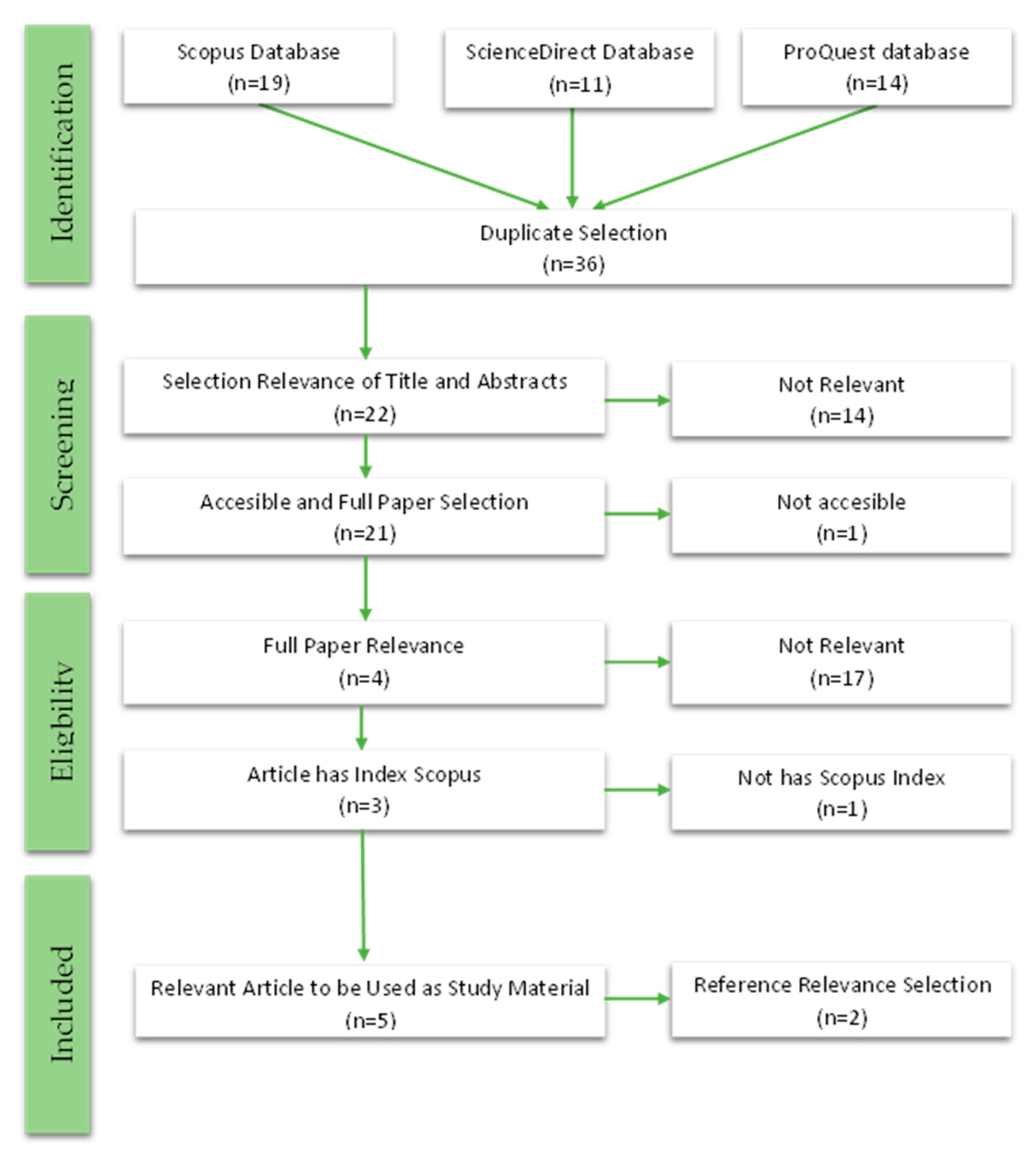
4.2. Searching Strategy

Articles published between 2000 and 2022 were identified using the search engines of the Scopus, ScienceDirect, and ProQuest databases. The keywords used in the search strategy can be seen in

Table 2. Numbers of articles obtained from Scopus, ScienceDirect, and ProQuest.

Stage	Keywords	Number of Articles
		Scopus	Science Direct	ProQuest
1	(“catastrophe bond” OR “CAT bond” OR “pricing cat bond” OR “valuation CAT bond”)	194	372	317
2	(“catastrophe bond” OR “cat bond” OR “pricing cat bond” OR “valuation CAT bond”) AND (“earthquake” OR “tsunamis”)	73	71	154
3	(“catastrophe bond” OR “CAT bond” OR “pricing CAT bond” OR “valuation CAT bond”) AND (“earthquake” OR “tsunamis”) AND (“extreme value theory”)	19	11	14

.

Table 2 shows that when the keywords “(“catastrophe bond” OR “CAT bond” OR “pricing cat bond” OR “valuation cat bond”) AND (“earthquake” OR “tsunamis”)” were used, data for 44 articles were obtained: 19 from the Scopus database, 11 from ScienceDirect, and 14 from ProQuest.

There were two steps to the selection process: one was semiautomatic, and the other was manual. First, duplicate articles were checked for on the Scopus, ScienceDirect, and ProQuest databases using the semiautomatic selection process; these duplicates were to be removed. We used the JabRef application to check for duplicate documents. After this, a manual selection process was used to find suitable articles for inclusion in the study. The inclusion and exclusion criteria used in this study are presented in

Table 3. The inclusion and exclusion criteria.

Inclusion criteria	I1	Articles discussing the pricing of catastrophe bonds
	I2	The developed model relates to earthquake disasters
	I3	Trigger modeling using extreme value theory
	I4	Articles in English
	I5	Articles published in a Scopus-indexed journal
Exclusion criteria	E1	Duplicate articles
	E2	Inaccessible articles

.

The phases of PRISMA are identification, screening, eligibility, and inclusion. In the identification phase, the exclusion criterion is duplicate articles (E1). In the screening phase, the exclusion criteria are the relevance of the abstract, title, and keywords. The phases of eligibility are divided into two-part steps that check the accessibility of the article (E2) and the relevance of the whole article to our research goals (I1, I2, I3, I4, I5). The flow of information through the different phases of PRISMA is presented in Figure 1.

Figure 1 shows that data were obtained from three reliable search engines: Scopus, ScienceDirect, and ProQuest. Therefore, 36 articles were screened after removal of duplicates. The next step was to filter articles relevant to the research topic. Fourteen articles were not suitable based on the relevance of their titles, abstracts, and keywords. One article was inaccessible, and seventeen did not link the catastrophe bond model to earthquakes based on the relevance of their full text. Moreover, one article was not indexed by Scopus. Thus, three articles were retained for use as primary studies.

A backward and forward process was carried out by collecting relevant citations from the three articles studied. This process was repeated and stopped when the article obtained was from the most recent year and there were no more cited articles. From this process, five articles were obtained that were relevant to the research topic [23,41,42,43,44].

Table 4. The summary of 23 articles based on accessibility and the relevance of their full text and references.

No	QR1	QR2	QR3	QR4	Description	Ref.
1	Developing a multi-period CAT bond pricing under uncertain conditions	Linear membership function, renewal process, ruin index, optimization model, and binary payoff function.	Indemnity	-	Not suitable	[45]
2	Creating a multi-period multiple-trigger CAT bond pricing model for coupon and zero-coupon bonds	ARIMA, Burr, generalized extreme value (GEV), Weibull, generalized Pareto (GPD), Log logistic, maximum likelihood estimation (MLE), nonhomogeneous Poisson process (NHPP), binary cash value function, Nuel recursive method (NRM), and Kolmogorov–Smirnoff	Modeled loss	Storm catastrophe in the United States	Not suitable	[25]
3	Developing a multi-hazard and multiregional CAT bond pricing	GEV, hydraulic flow model, and Monte Carlo simulation	Parametric	Flood in Oregon, US	Not suitable	[26]
4	Introducing a CAT bond pricing for a single period with coupon payments in Romania	Linear piecewise payoff function, GEV, block maxima method (BMM), and maximum likelihood estimation (MLE)	Parametric	Earthquake in Romania	Not suitable	[13]
5	Developing a framework for valuing multi-period multi-risk reinsurance contract	Poisson, CIR, GPD, MLE, copula, Kolmogorov–Smirnov, sensitivity analysis, and Monte Carlo simulation	Modeled loss	Simulation data of flood reinsurance	Not suitable	[27]
6	Studying the pricing of multi-period drought CAT bonds by the POT model and high quantile estimation	Kurtosis method, the static term structure of interest rates, the binary payoff function, the Poisson process, GPD, Lagrangian, and MLE	Modeled loss	Drought catastrophe for 21 countries	Not suitable	[28]
7	Developing multi-period CAT bond pricing for multiple event catastrophe bonds based on CIR, copula, and POT models	Poisson process, binary payoff function, CIR, peaks over threshold, GPD, copula, Monte Carlo simulation, sensitivity analysis to determine the impact of catastrophe intensity, maturity date, and the dependence on catastrophe bond prices	Modeled loss	-	Not suitable	[29]
8	Developing multi-period CAT bond pricing considering risk credit	Linear piecewise payoff function, probability of default, GEV, and MLE	Industry loss	USA catastrophe	Not suitable	[46]
9	Developing explicit multi-period CAT bond prices in terms of four different payoff functions	CIR, compound Poisson, semi-Markovian dependence structure in continuous time, binary and piecewise payoff function, GEV	Industry loss	USA catastrophe	Not suitable	[14]
10	Analyzing the securitization of longevity risk, with an emphasis on longevity risk modeling and longevity bond premium pricing	Option payoff function, mortality index model, the classic Lee–Carter model, singular value decomposition, random walk model with drift, normal distribution, EVT to model tail distribution, premium spread model, conditional expected loss, Cobb–Douglass function to capture the tradeoff between CEL and PFL, and the Lane Financial Corporation (LFC) cubic model	Mortality index	-	Not suitable	[47]
11	Developing multi-period CAT bond pricing with and without coupons	CIR, Poisson process, compound Poisson process, binary payoff function, nonhomogeneous Poisson process, fast Fourier transform, inversion method, approximation method, recursive method, gamma, skewness, GEV	Industry loss	US catastrophe	Not suitable	[48]
12	Valuation of a CAT mortality bonds model	Mortality index model, linear piecewise payoff function, binary payoff function t, the proportion of the principal returned model, and a discounted cash flow model	Mortality index	-	Not suitable	[49]
13	Developing a framework for multi-period pricing of data breach CAT bonds	Linear piecewise payoff function, equilibrium pricing theory, GEV, MLE, Akaike information criterion (AIC), and negative likelihood	Industry loss	-	Not suitable	[50]
14	Developing multi-period CAT bond pricing with coupons to propose a mathematical formulation for the probability that the incurred losses exceed a certain threshold D before the bonds’ expiration	Compound Poisson process and CIR	Modeled loss	-	Not suitable	[51]
15	Developing multi-period CAT bond pricing based on a product pricing measure combined with a distorted probability function	GEV, GPD, MLE, and R function, Vasicek, sensitivity analysis, and Wang transformation	Parametric	Californian earthquake	Referencepaper	[44]
16	Developing a pricing model for multi-period CAT bond premiums	Linear piecewise payoff function, expected loss model, correlation test, value at risk (VaR), conditional tail expectation, EVT, asymptotic analysis, MLE, GEV, and GPD	Modeled loss	Wildfire Fort McMurray, Canada	Not suitable	[52]
17	Modeling multi-period CAT bond pricing	Hull–White, NHPP, compound Poisson process, doubly stochastic process, GPD, maximum likelihood, and numerical optimization	Industry loss	US catastrophe	Not suitable	[53]
18	Modeling CAT bond pricing with a temperature based on agriculture	Utility without catastrophe risk bond model, utility with and without catastrophe risk bond model, and ask-and-bid price model	Parametric	Agriculture in Iran	Not suitable	[54]
19	Developing Cox and Pederson [55] single- and multi-period CAT bond pricing models with multiple catastrophes and risks	Linear piecewise payoff function, ARIMA (1, 1, 1), CIR, block maxima, GEV, and gamma	Parametric	Californian earthquake	Referencepaper	[43]
20	Creating single- and multi-period CAT bond pricing for the earthquakes in the Greek border area	Log-normality, CIR, linear piecewise payoff function, GEV, MLE, and the FORTRAN subroutine MLEGEV	Parametric	Greek earthquakes	Referencepaper	[23]
21	Modeling of left-truncated heavy-tailed data for application to catastrophe bond pricing	Compound Poisson process, NHPP, naïve approach, shifting approach, conditional complete data (CCD), MLE, maximum product of spacing (MPS), goodness-of-fit test, Moran’s log spacing statistic, Burr, GPD, and GEV	Industry loss	-	Not suitable	[56]
22	Analyzing multi-period CAT bonds with and without coupons	Homogeneous Poisson process (HPP), NHPP, continuous compound interest, binary payoff function, regression analysis, mean excess function, mean absolute difference (MAD), mean absolute values’ relative differences (MAVRD), Log-normal, Pareto, Burr, exponential, gamma, and Weibull	Hybrid trigger (modeled index losses)	Mexican earthquake	Reference paper	[41]
23	Developing multi-period hybrid CAT bonds with coupons	Poisson distribution, Poisson process, binary payoff function, POT, GPD, Archimedean copula, CIR, and continuous compound interest	Hybrid trigger (modeled losses and parametric)	Losses and their magnitude in China	Reference paper	[42]

shows the complete review of 23 articles based on accessibility, full-text selection, and reference relevance.

4.3. Analysis Data

4.3.1. Overviews of Previous Models

Tang and Yuan [44] developed a multi-period earthquake bond pricing model with coupons based on pricing measures and a distorted probability function. The study used the Poisson process to determine the number of disaster events at time t, while GEV and GPD were used to model the maximum annual loss caused by the earthquake. Moreover, MLE and the R function were used to estimate the parameters in the GEV and GPD distributions. Vasicek was employed to model risk-free interest and coupons, while Wang’s transformation was used to model the pricing of premium disaster bonds. The study also used the modeled loss trigger designed using a compound Poisson process based on frequency and severity. However, the probability measure was distorted based on severity alone.

Shao et al. [43] developed a Cox–Pederson catastrophe bond pricing model [55] and associated it with single- and multi-period earthquake disasters. The model used in the payment function was a linear piecewise function. The study modeled the interest rates and inflation using ARIMA (1, 1, 1), while CIR was used to model the coupons. Furthermore, block maxima were used to determine the maximum annual earthquake magnitude. GEV was employed to model the distribution of the magnitude of the annual earthquake disasters, while gamma distribution was used to model the depth of the earthquakes. The study used a parametric trigger, implying the magnitude and depth of an earthquake in California.

Zimbidis et al. [23] developed a single- and multi-period earthquake bond pricing model for the Greek area. The study used a Log-normal distribution to model the year-end deposit interest rate and a CIR to model coupons based on annual EURIBOR. GEV was used to model the maximum annual earthquake magnitude, while MLE and the FORTRAN subroutine MLEGEV were used to estimate the parameters of the GEV distribution.

Hardle and Carbera [41] analyzed multi-period CAT bonds with coupons for earthquakes in Mexico. The study used a homogeneous Poisson process (HPP) with exponentially distributed intensity to model the arrival process of an earthquake, a nonhomogeneous Poisson process (NHPP) to determine aggregate loss, a Poisson process to determine the intensity of natural events, and continuous compound interest to calculate interest and coupon rates. The coupon used was constant and equal to LIBOR in May 2006. The study assumed fixed quarterly coupon payments. The data used were from earthquakes that occurred in Mexico. The authors analyzed the effects of magnitude, depth, and Log-magnitude on the economic losses caused by the earthquake disaster in Mexico. The coefficient of determination was 0.15 for data in 1985 and 0.129 for data in 1989 and 1999. Thus, the authors used the mean excess function to find an accurate loss distribution. Because the losses had heavy tails, they used Log-normal, Pareto, Burr, exponential, gamma, and Weibull distributions to model loss data. The MAD and MAVRD were used to determine the impact of the loss model on zero CAT bond prices. The results were modeled-index CAT bonds that reduce the basis and the moral risk borne.

Wei et al. [42] developed a pricing model for hybrid-trigger catastrophe bonds. The Poisson distribution was used to model disaster intensity, the Poisson process was used to determine the probability of the number of earthquakes, and the binary function was used to model cash flows to bondholders at a given time. The study used the POT model to collect data on earthquake magnitude and losses as a result of the earthquake disaster, GPD to model magnitude and loss distribution, Archimedean copula to model the dependence and joint distribution of magnitude and loss, CIR to model interest rates and coupons, continuous compound interest to determine the interest and coupon rates, VaR to determine maximum losses, analysis of the effect of the trigger on CAT bond prices, and analysis of the effects of interest rates and coupon rates. The data were used to simulate the magnitude and losses due to earthquakes in China from 1990 to 2020. The numerical experiment showed that the maturity, trigger level, dependence of trigger indicators, and financial risk (i.e., interest and coupon rates) affected the CAT bond price. The models discussed in the primary study are represented in

Table 5. Previous earthquake catastrophe bond pricing model.

Model 1 [44]	$\begin{array}{ll}{P}_t=& K{E}_t^{Q^1}\left({\displaystyle \sum _{s=\lfloor t\rfloor +1}^{\lfloor \tau \rfloor \Lambda T}}\Pi \left(Y_{s-1}\right)E_t^{Q^2}\left(D\left(t,s\right)\left(R+i_s\right)\right) \right)+\\ & K{E}_t^{Q^1}\left(\left(\tau -\lfloor \tau \rfloor \right)\Pi \left(Y_{\lfloor \tau \rfloor }\right)1_{\left(\tau \le T\right)}{E}_t^{Q^2}\left(\left(D(t,\tau \right)\left(R+i_{\tau }\right)\right)+K{E}_t^{Q^1}\left(D\left(t,T\right)\Pi \left(Y_T\right)\right)\right)\end{array}$
Model 2 [43]	Single-Period Model $V\left(d\right)=\frac{1}{1+\left(r+e\right)}.\frac{1}{1+\pi }.E^P(d\left(R;M,D\right)$ $d\left(R;M,D\right)=\{\begin{array}{cc}K.\left(1+f\left(R\right)\right)& M\in \left[0,{\mu }_1\right],\mathrm{with} \left(D\le {\delta }_1\right) \mathrm{or} \left(\mathrm{D}>{\mathsf{\delta }}_1\right)\\ K.\left(1+g\left(R\right)\right)& M\in \left[{\mu }_1,{\mu }_2\right],\mathrm{with} \left(D\le {\delta }_2\right) \mathrm{or} (\mathrm{D}>{\mathsf{\delta }}_2)\\ K.\left(1+h\left(R\right)\right)& M\in \left[{\mu }_2,{\mu }_3\right],\mathrm{with} \left(D\le {\delta }_3\right) \mathrm{or} (\mathrm{D}>{\mathsf{\delta }}_4)\\ K& M\in \left[{\mu }_3,{\mu }_4\right]\\ \varphi \left(K\right)& M\in \left[{\mu }_4,{\mu }_5\right],\mathrm{with} \left(D\le {\delta }_4\right) \mathrm{or} (\mathrm{D}>{\mathsf{\delta }}_4)\\ \gamma \left(K\right)& M\in \left[{\mu }_6,{\mu }_7\right],\mathrm{with} \left(D\le {\delta }_5\right) \mathrm{or} (\mathrm{D}>{\mathsf{\delta }}_5)\\ \eta \left(K\right)& M\in \left({\mu }_6,\infty \right)\end{array}$ Multi-Period Model $V{\left(d\right)}^h=\frac{1}{h}\sum _{l=1}^h\sum _{k=1}^T\frac{1}{{\prod }_{s=0}^{k-1}\left(1+r_s^l+e)(1+{\pi }_s^l\right)}\overline{d}\left(R_k^l;M_k^l,D_k^l\right)$ $d\left(R_k;M_k,D_k\right)=\{\begin{array}{l}Kf\left(R_k\right){\mathbf{1}}_{0\le M_k\le {\mu }_1}+Kg\left(R_k\right){\mathbf{1}}_{{\mu }_1<M_k\le {\mu }_2}+Kh\left(R_k\right){\mathbf{1}}_{{\mu }_2<M_k\le {\mu }_3},k=1,2,\dots ,T-1\\ K\left(1+f\left(R_k\right)\right){\mathbf{1}}_{0\le M_k\le {\mu }_1}+K\left(1+g\left(R_k\right)\right){\mathbf{1}}_{{\mu }_1<M_k\le {\mu }_2}+K(1+h\left(R_k\right){\mathbf{1}}_{{\mu }_2<M_k\le {\mu }_3}\\ +K{\mathbf{1}}_{{\mu }_3<M_k\le {\mu }_4}+\varphi \left(K\right){\mathbf{1}}_{{\mu }_4<M_k\le {\mu }_5}+\gamma \left(K\right){\mathbf{1}}_{{\mu }_5<M_k\le {\mu }_6}+\eta \left(K\right){\mathbf{1}}_{M_k>{\mu }_6}, for k=T\end{array}$ $\overline{d}\left(R_k;M_k,D_k\right)=\{\begin{array}{c}{E}^Q\left(Kf\left(R_k\right){\mathbf{1}}_{0\le M_k\le {\mu }_1}+Kg\left(R_k\right){\mathbf{1}}_{{\mu }_1<M_k\le {\mu }_2}+Kh\left(R_k\right){\mathbf{1}}_{{\mu }_2<M_k\le {\mu }_3}\right),k=1,2,\dots ,T-1\\ E^Q(K\left(1+f\left(R_k\right)\right){\mathbf{1}}_{0\le M_k\le {\mu }_1}+K\left(1+g\left(R_k\right)\right){\mathbf{1}}_{{\mu }_1<M_k\le {\mu }_2}+K(1+h\left(R_k\right){\mathbf{1}}_{{\mu }_2<M_k\le {\mu }_3}\\ +K{\mathbf{1}}_{{\mu }_3<M_k\le {\mu }_4}+\varphi \left(K\right){\mathbf{1}}_{{\mu }_4<M_k\le {\mu }_5}+\gamma \left(K\right){\mathbf{1}}_{{\mu }_5<M_k\le {\mu }_6}+\eta \left(K\right){\mathbf{1}}_{M_k>{\mu }_6}), for k=T\end{array}$
Model 3 [23]	Single-Period $P=E_{Q_1}\left(e^{-\left(r+e\right)}C\left(M\right)\right)$ $C\left(M\right)=\{\begin{array}{cc}K\left(1+3R\right)& M\in \left(0, 5.4\right]\\ K\left(1+2R\right)& M\in \left(5.4, 5.8\right]\\ K\left(1+R\right)& M\in \left(5.8, 6.2\right]\\ K& M\in \left(6.2, 6.6\right]\\ 2/3K& M\in \left(6.6, 7\right]\\ 1/3K& M\in \left(7, 7.4\right]\\ 0& M\in \left(7.4 \infty \right)\end{array}$ Multi-Period $P^m=e^{-\left(r+e\right)T}\left(\frac{1}{m}\right)\sum _{j=1}^m\sum _{l=1}^{T}F{V}_T\left(R_l^{\left(j\right)},M_l^{\left(j\right)}\right)$ $F{V}_{T}f\left(R_l,M_l\right)=f\left(R_l,M_l\right)\prod _{k=0}^{T-l-1}\left(i+i_{l+k}\right)$ $f\left(R_l,M_l\right)=\{\begin{array}{c}\left(3R_l\right){\mathbf{1}}_{\left[0<M_1\le 5.4\right]}+\left(2R_l\right){\mathbf{1}}_{\left[5.4<M_1\le 5.8\right]}+\left(R_l\right).{\mathbf{1}}_{\left[5.8<M_1\le 6.2\right]},\\ l=1,2,\dots ,T-1\\ \left(3R_l\right){\mathbf{1}}_{\left[0<M_1\le 5.4\right]}+\left(2R_l\right){\mathbf{1}}_{\left[5.4<M_1\le 5.8\right]}+\left(R_l\right).{\mathbf{1}}_{\left[5.8<M_1\le 6.2\right]}+K.{\mathbf{1}}_{\left[5<\max (M_1)\le 6.6\right]}\\ K.{\mathbf{1}}_{\left[5<\max (M_1)\le 6.6\right]}+\frac{2}{3}K.{\mathbf{1}}_{\left[6.6<\max (M_1)\le 7\right]}+\frac{1}{3}K.{\mathbf{1}}_{\left[7<\max (M_1)\le 7.4\right]},l=T\end{array}$
Model 4 [41]	Zero-Coupon Bond $V_t^1=E\left(P{e}^{-R\left(t,T\right)}\left(1-M_T\right)|{ℱ}_t\right)$ $\mathsf{\tau }=inf\left(t:L_t\ge D\right)$ Coupon Bond $V_t^2=E\left(P{e}^{-\left(R\left(t,T\right)\right)}\left(1-M_T\right)+{\int }_t^T{e}^{R\left(t,s\right)}{C}_s\left(1-M_s\right)ds|{ℱ}_t\right)$ $\tau =inf\left(t:L_t\ge D\right)$
Model 5 [42]	$P=F\left(R{\displaystyle \sum _{t=1}^T}{\left(1-v_c\right)}^{t}p\left(0,t\right)+\left(1-v_F\right)p\left(0,T\right)\right)$ $CF\left(t\right)=\{\begin{array}{cc}FR{\mathbb{I}}_{{\tau }_C>t }& t=1,2,\dots ,T-1\\ FR{\mathbb{I}}_{{\tau }_C>t }+F{\mathbb{I}}_{{\tau }_F>t}& t=T\end{array}$

.

The earthquake bond pricing model developed by Tang and Yuan [44] measures the expected price uncertainty, the payment function’s discounted value, information on trigger developments, and financial market performance over time $t\in \left[0, T\right]$. The assumptions used in the trigger model are a nonnegative, non-decreasing, and right-continuous stochastic process, defined as follows:

$$Y_t={\displaystyle \sum }_{j=1}^{N_t}{1}_{X_j>y},t\ge 0$$

(1)

where $N_t$ is the number of earthquakes modeled by the Poisson process up to time $t, X_j$ is the $j$-th earthquake’s magnitude, $y$ is the threshold, and $1_{\Delta }$ is an indicator of the occurrence of earthquakes, with a value of 1 when $\Delta$ occurs and 0 otherwise. $X_j$ can be modeled using the GEV or GPD distribution. The cash payment value depends on trigger $Y$ in the time interval $\left[0,t\right]$, defined as $\Pi (.):\left[0,\infty \right)\to \left[0,1\right]$, which is a non-decreasing and continuous function with $\Pi \left(.0\right)=1$, meaning that at any time $t\in \left[0, T\right]$ the cash value of the disaster bond is $K\Pi \left(Y_t\right)$. Therefore, a trigger would delete several cash values of $K\Pi \left(Y_{t-0}\right)-K\Pi \left(Y_t\right)$, where $Y_{t-0}$ is the value of $Y$ before time $t$, and $Y_t$ is the value of $Y$ if an earthquake occurs. The cash value function obtained by bondholders is formulated as follows:

$$K\left(R+i_t\right)\Pi \left(Y_{t-1}\right)$$

(2)

The cash value in Equation (2) represents the coupon at time $t=1,\dots , T$ and the face value $K\Pi \left(Y_{t-1}\right)$ at maturity when no trigger occurs. The trigger functions are as follows:

$$\tau =inf\left(t\in R_{+}:\Pi \left(Y_t\right)=0\right)$$

(3)

When the trigger occurs between two coupon dates, bondholders receive the proportion of coupons received before the trigger, calculated as follows:

$$\vartheta =\left(\tau -\lfloor \tau \rfloor \right)\left(R+i_{\tau }\right)\Pi \left(Y_{\lfloor \tau \rfloor }\right),$$

(4)

where $\lfloor .\rfloor$ is a floor function, and the amount of cash value to be obtained by bondholders is $K\vartheta . D(t,s)$ is the discount factor associated with the interval $\left[t,s\right]$, while $D\left(t,s\right)=e^{-{\int }_t^s{r}_{u}du}$, $i_t$ is a floating coupon per year, $R$ is a fixed coupon per year, $r_t$ is the risk-free interest rate at time $t$ for $t\ge 0, E_t^{Q^1}$ is the expected yield obtained by the earthquake catastrophe bondholders, and $E_t^{Q^2}$ is the expected coupon size and discount factor.

The notations in the work of Shao et al. [43] are as follows: $K$ is the principal value of the earthquake catastrophe bond,$r$ is the real risk-free interest rate for one period, and $\pi$ is the inflation rate for one period. Furthermore, $R$ was used as the coupon rate for one period (using US LIBOR for 12 months), and $M$ was used as the maximum earthquake magnitude in an area. When two earthquakes occur simultaneously, $M=max\left(M^1, M^2\right)$, where $M^1$ and $M^2$ represent the earthquake’s magnitude in each region, $D$ is the earthquake’s depth, and $v\left(D\right)$ is the issue price of the earthquake catastrophe bond. Moreover, $d\left(R; M, D\right)$ is a payoff function; $T$ is a time maturity; $r_k$ is the market yield using the 1-year treasury security rate at time $k$, following the ARIMA (1, 1, 1); ${\pi }_k$ is the 1-year inflation rate at time $k$, following the ARIMA (1, 0, 0); $R_k$ is a coupon rate, modeled using CIR based on 12-month LIBOR at time $k; M_k$ is the maximum annual earthquake magnitude in the $n$-th year; $k=1,2,\dots , T$; and $M_k=max\left\{M_k^1, M_k^2\right\}$ for $k=1,2,\dots , T$. In this case, $M_k^1$ and $M_k^2$ have GEV distribution, $D_k$ is the depth and magnitude in year $t$, $d\left(R_k,M_k, D_k\right)$ is the payoff function that bondholders receive at $k=1,2,\dots , T$, and $\overline{d}\left(R_k;M_k, D_k\right)$ is the expected payoff function.

The notations in the work of Zimbidis et al. [23] are as follows: $E\left(Q_1\right)$ is the expected present value of the cash value associated with the probability of an earthquake; $r$ is the risk-free interest rate; $e$ is the extra premium; $C\left(M\right)$ is the payoff function; and $K$ is the cash value. The notations $K, r,$ and $e$ in the multi-period model are the same as in the single-period model. Furthermore, $T$ is the maturity time; $i_n$ is the interest rate, assumed to follow a Log-normal distribution; $R_t$ is the coupon rate modeled using CIR; $R^j$ is the $j$-th path (realization) of the EURIBOR level $(R_t,t\in \left[0, T\right]\}$; $M_n$ is the maximum earthquake magnitude in Greece in the $n$th year; $M^j$ is the jth path (realization) of $\left(M_n,n=1,2,\dots \right)$ for the maximum earthquake magnitude per year; and $f\left(R_l, M_l\right)$ is the cash value obtained by earthquake catastrophe bondholders at time $l=1,2,\dots , T.$

The assumptions in the zero-coupon [41] that pays a principal amount at time maturity $T$ are as follows: a threshold time event $\tau =inf\left(t:L_t\ge D\right)$ is the moment when the aggregate loss $L_t$ exceeds the threshold level $D$; ${ℱ}_t$ is the increase in filtration with time $t\in \left[0,T\right]$; $e^{-\left(R\left(t,T\right)\right)}=e^{-{\int }_s^{t}r\left(\xi \right)d\xi }$ is a continously compounded discount interest rate; $V_t^1$ is a zero-coupon bond price; and $M_t=1\left(L_t>D\right)$ is the threshold time as a doubly stochastic Poisson process. The assumptions in the coupon bond that pays the principal $P$ at time to maturity $T$ give a coupon $C_s$ with a fixed spread $z$ until the threshold time $\tau$, $M_T$, and $e^{-\left(R\left(t,T\right)\right)}$ are the same as the zero-coupon model.

Wei et al. [42] developed a hybrid-triggered CAT bond; the notations in the model were as follows: $N_t$ denotes the number of earthquake disasters that occurred between $\left(t-1,t\right),$ $d_i,i=1,2,3,\dots ,m \left(m=\sum _{t=1}^T{N}_t\right)$ (i.e., occurrence time of the $i$-th earthquake); the economic loss caused by the earthquake disaster is denoted by $X_d,d=d_1,d_2,\dots ,d_m$; the magnitude of earthquake disaster that occurred at time $d$ is denoted by $Y_d,d=d_1,d_2,\dots ,d_m$; $CF\left(t\right)$ is the cash value at time $t$; the principal’s payoff structure is $F{\mathbb{I}}_{{\tau }_F>t}$; $FR{\mathbb{I}}_{{\tau }_C>t }$ is the structure of the coupon; ${\tau }_C=min(d=d_1,d_2,\dots ,d_m|X_d>T{r}_X or Y_d>T{r}_Y)$ is the first time when the economic loss exceeds $T{r}_X$ or the magnitude exceeds $T{r}_Y$; ${\tau }_F=min(d=d_1,d_2,\dots ,d_m|X_d>T{r}_X and Y_d>T{r}_Y)$ is the stopping time as the first time when the economic loss exceeds $T{r}_X$ or the magnitude exceeds $T{r}_Y$; $v_c$ is the probability that trigger condition for the coupon is satisfied in the interval $\left[t-1,t\right]$; $v_F$ is the probability that the trigger condition for the principal is satisfied in the interval $\left[0,T\right]$; $p\left(0,t\right)=A\left(0,t\right)e^{-B\left(0,t\right)r}$ is the price of a non-defaultable zero-coupon bond with a face value of 1 maturing at a time $t$, where $A\left(0,t\right)={\left(\frac{2\eta e^{\frac{\left(\kappa +\eta \right)t}{2}}}{\left(\kappa +\eta \right)\left(e^{\eta t}-1\right)+2\eta }\right)}^{\frac{2\kappa \theta }{{\epsilon }^2}}$, $B\left(0,t\right)=\frac{2\left(e^{\eta t}-1\right)}{\left(\kappa +\eta \right)\left(e^{\eta t}-1\right)+2\eta },\eta =\sqrt{{\kappa }^2+2{\epsilon }^2}$; $\kappa >0$ is the mean reverting force measurement, $\epsilon >0$ is the votality parameter, $\theta >0$ is the long-term mean of the interest rate, r is the initial interest rate, ${\mathbb{I}}_{(.)}$ is an indicator function, $F$ is the face value, and $R$ is the coupon rate.

4.3.2. Comparison of Previous Models

The description in Section 4.3.1 implies that triggering distribution modeling for earthquake catastrophe bond prices entails utilizing GEV, GPD, Burr, Log-normal, or gamma; using the Poisson process to estimate the number of earthquake catastrophes up to time t; NHPP to determine the aggregate loss; Archimedean copula (AC) to model the dependency of joint distribution losses and the magnitude of earthquakes; Log-normal, CIR, ARIMA, and Vasicek to model the financial risk; and binary and linear piecewise functions to model payoff.

Table 6. Summary of the trigger parameters used in primary studies.

Author	Trigger Parameter
	Magnitude	Depth	Losses	Aggregate Losses
Tang and Yuan [44]	√	-	-	-
Shao et al. [43]	√	√	-	-
Zimbidis et al. [23]	√	-	-	-
Hardle and Carbera [41]	-	-	-	√
Wei et al. [42]	√	-	√	-

summarizes the five chosen papers’ techniques and models for earthquake catastrophe bond pricing.

Table 6 shows that the trigger types used are parametric and hybrid triggers. Tang and Yuan [44] and Zimbidis et al. [23] used earthquake magnitude, Shao et al. [43] used earthquake depth and magnitude, Hardle and Carbera [41] used aggregate loss, and Wei et al. [42] used the magnitude of the earthquake and the losses caused by the disaster.

Table 7. Summary of the trigger distribution models used in primary studies.

Author	Trigger Distribution
	GEV	GPD	Gamma	AC	NHPP	Burr	Log-Normal
Tang and Yuan [44]	√	√	-	-	-	-	-
Shao et al. [43]	√	-	√	-	-	-	-
Zimbidis et al. [23]	√	-	-	-	-	-	-
Hardle and Carbera [41]	-	√	-	-	√	√	√
Wei et al. [42]	-	√	-	√	-	-	-

shows that Tang and Yuan [44] used GEV and GPD to model the distribution of earthquake magnitude. Shao et al. [43] used GEV to model earthquake magnitude and GPD to model earthquake depth. Zimbidis et al. [23] and Hardle and Carbera [41] used GPD, Burr, and Log-normal to model losses due to earthquake disasters, and they used NHPP to model the aggregate loss distribution. Wei et al. [42] used GPD to model losses and earthquake magnitude distribution, and they used AC to model the dependency of magnitude and loss distribution.

Table 8. Summary of financial risk model used in primary study.

Author	Financial Risk Model
	Log-Normal	Vasicek	ARIMA	CIR	Constant
Tang and Yuan [44]	-	√	-	-	-
Shao et al. [43]	-	-	√	√	-
Zimbidis et al. [23]	√	-	-	√	-
Hardle and Carbera [41]	-	-	-	-	√
Wei et al. [42]	-	-	-	√	-

shows that Tang and Yuan [44] used Vasicek to model the interest and coupon rate. Shao et al. [43] used ARIMA to model interest rates and inflation, and they used CIR to model the coupon rate. Zimbidis et al. [23] used Log-normality to model the interest rate and CIR to model the coupon rate. Hardle and Carbera [41] used constant interest and coupon rates. Wei et al. [42] used CIR to model the interest and coupon rates.

Table 9. Summary of the payoff function models used in primary studies.

Author	Payoff Function
	Binary	Piecewise
Tang and Yuan [44]	√	-
Shao et al. [43]	-	√
Zimbidis et al. [23]	-	√
Hardle and Carbera [41]	√	-
Wei et al. [42]	√	-

shows that [41,42,44] used binary functions to model payoff, while [23,43] used linear piecewise payoff functions.

4.3.3. Literature Gap

The limitations of the ECBPM in the five selected articles are described as follows:

(a)

Earthquake magnitude triggers [23,44] have not been used to describe the earthquake disaster severity [57].

(b)

The earthquake severity depends on its location, magnitude, and depth, which are not discussed in the five selected articles.

(c)

Earthquake magnitude distribution modeled using GEV can eliminate extreme data for a period [29].

(d)

The modeling of interest and coupon rates using the Vasicek model [44] allows negative values. The volatility of interest rate changes is assumed to be constant and unrealistic for bond prices [58].

(e)

Modeling of interest rates and inflation using ARIMA [43] allows negative values [59].

(f)

The coupon rate modeled using CIR is better than that using the Vasicek model [44]. However, it has constant volatility and no jump caused by monetary policy [58].

(g)

Discussion of the Poisson process can be found in [41,42,44] for determining the number of earthquake events at a time t. This is considered necessary in modeling to determine a trigger’s probability of occurring at time t.

(h)

The payoff function is modeled using a binary function in [41,42,44], while [23,43] use a linear piecewise payoff function. The linear piecewise modeling is better than a binary function because it can describe the level of losses due to earthquakes.

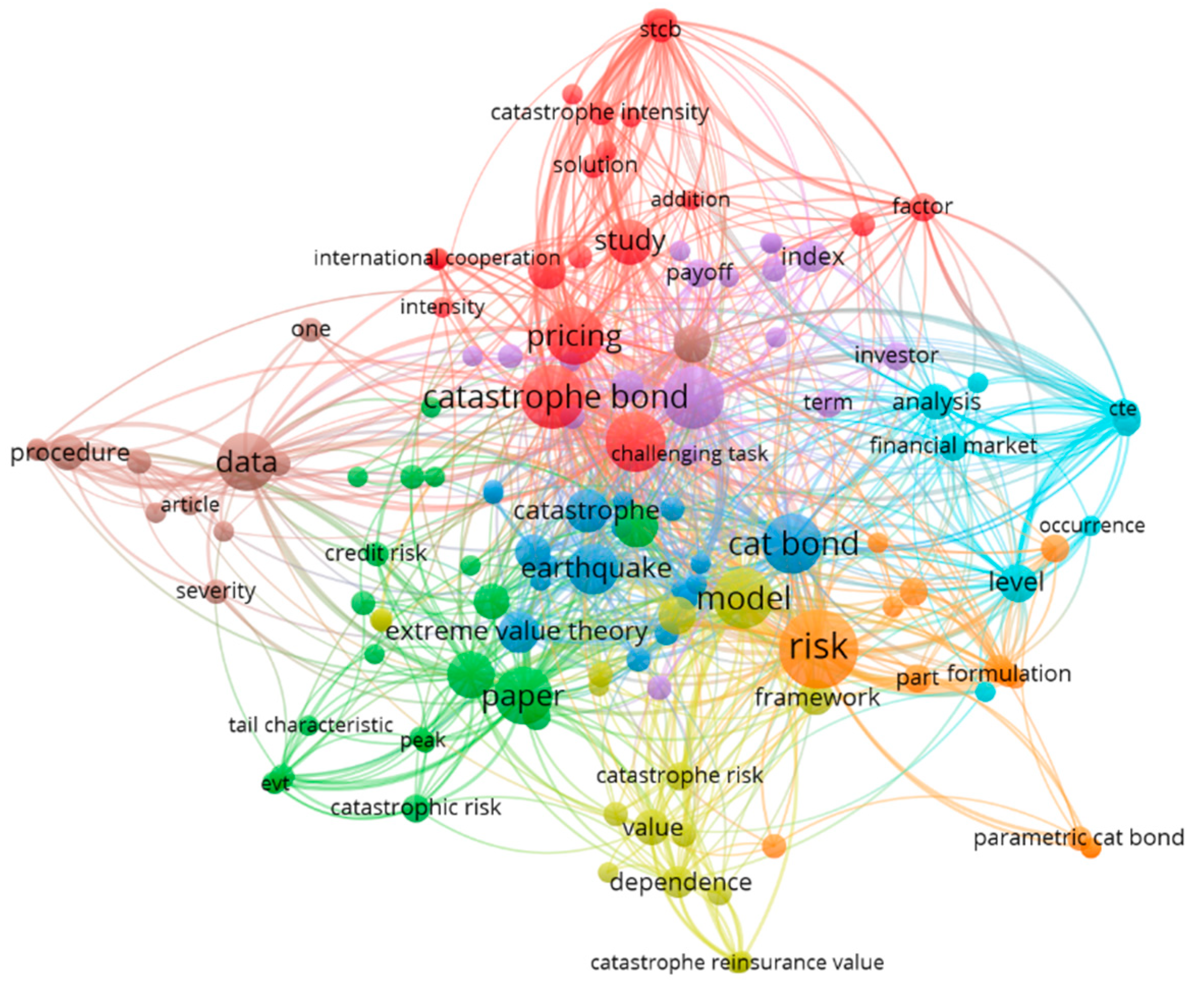
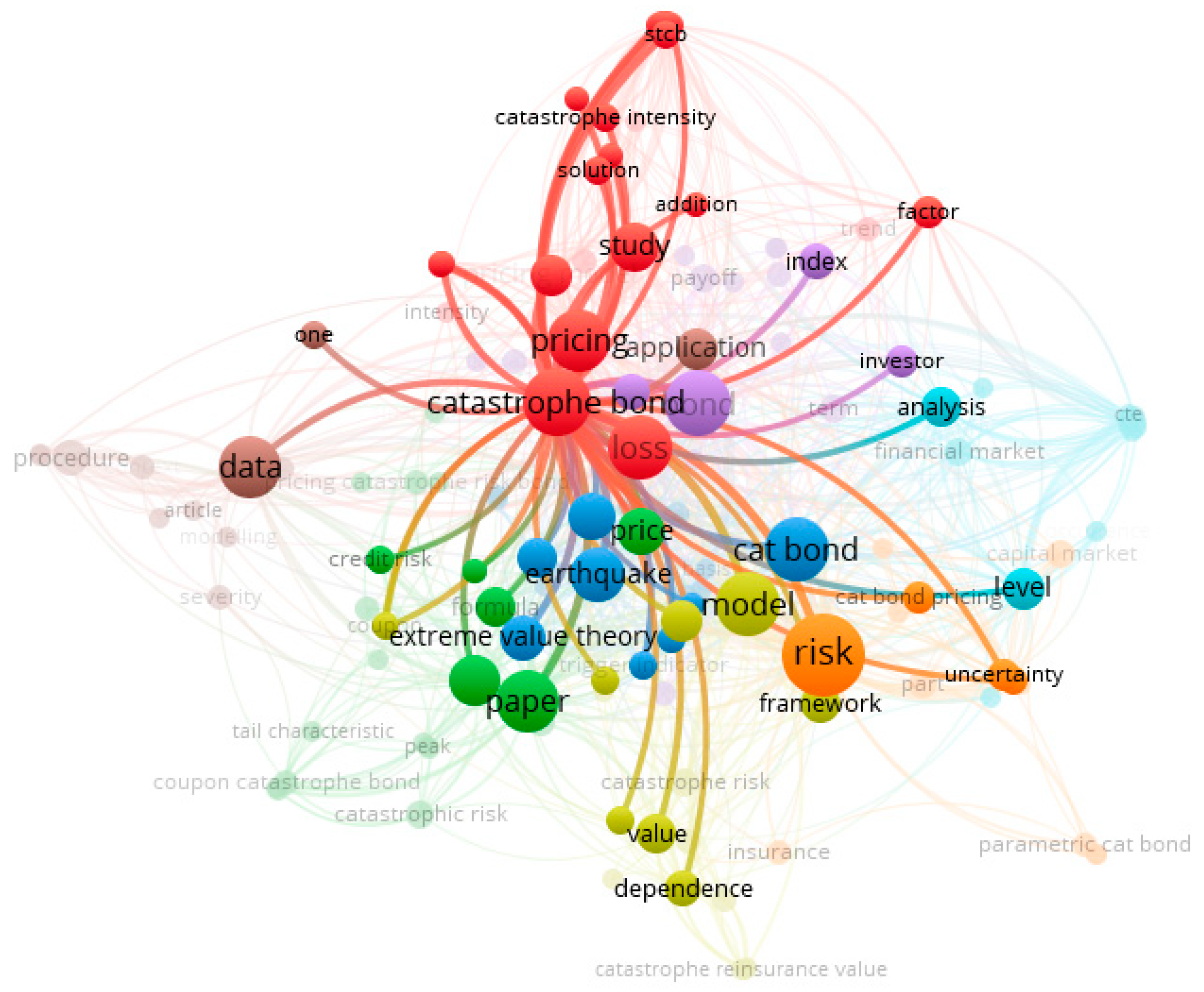
4.4. Bibliometric Analysis

About 23 articles were relevant to the keywords used, as described in Table 4. They were selected based on accessibility and the relevance of their full text and references. Figure 2 shows the results of visualizing the bibliometric network using the VOSviewer application.

There are several nodes with various sizes and distances. The amount of words discussed is indicated by the size of the node. Furthermore, the number of terms in the database increases with node size. The distance between each node reveals the degree of the connections between the words. Figure 2 shows that the distance from the earthquake and EVT to catastrophe bond pricing is quite far, despite the modest size of the earthquake and EVT node. In addition, the distance from copula and analysis to earthquake and catastrophe bond is far.

Figure 3 shows no relationship between the earthquake catastrophe bond pricing model and regional grouping. In addition, there are no nodes that state the fuzzy time series and ECIR to model interest rates and inflation. The findings obtained open up opportunities for the development of a model to determine the price of earthquake bonds.

5. Discussion

The extreme value theory in earthquake catastrophe bond pricing models extreme data from earthquake magnitude and losses due to earthquake disasters. The high earthquake magnitude or losses are obtained using the block maxima method (BMM). This involves selecting extreme data per month, quarter, semester, or year. The process could also use peaks over the threshold (POT) by choosing an extreme value greater than the threshold value. The extreme values obtained using BMM follow the GEV distribution [18]). In contrast, the extreme values obtained using POT follow the GPD distribution [29]). The parameters in GEV are location, scale, and shape, while in GPD they are only scale and shape. The parameter estimation uses the MLE method, in which the maximum value of the likelihood function in the parameter results in a closed form, which requires numerical methods to solve.

Zimbidis et al. [23] investigated the concept of ECBPM in 2007 and found that only five articles in Scopus-indexed journals addressed pricing models for earthquake catastrophe bonds utilizing EVT. However, many studies have worked on constructing catastrophe bond models. The five articles in question only developed models for the payment function, financial market risk, and trigger distribution, each with advantages and disadvantages. The trigger type created by Tang and Yuan [44] uses several variables, including earthquake depth and magnitude. However, it does not describe the joint probability distribution of the two parameters. Since inflation impacts catastrophe bond prices, only Shao et al. [43] discussed the inflation variable and modeled inflation using ARIMA. This method allows negative values [59]. The Vasicek model [44] is inferior to CIR interest rate modeling. Therefore, the CIR model must be improved to address the ongoing volatility and leaps caused by monetary policy. GPD is superior to GEV for modeling earthquake magnitude.

Tang and Yuan [44] performed sensitivity analysis of the location and shape parameters. This was insufficient, because bond prices are significantly influenced by interest and coupon rates, maturity, and inflation. Hardle and Carbera [41] analyzed the robustness of the various loss models, finding that the bond prices are more dispersed under various expected loss models with the same distribution assumption than under various distribution assumptions with the same loss model. Wei et al. [42] analyzed the effects of different maturity periods, dependencies, interest rates, and coupon rates on catastrophe bond prices. The results were as follows: the greater the maturity, the cheaper the price of the disaster bond; the greater the dependency, the cheaper the price of disaster bonds; interest rates are inversely related to bond prices; and the higher the coupon rate, the higher the price of disaster bonds. In addition, increasing the trigger level causes the probability of triggering events to be smaller. The analysis carried out on the three articles [41,42,44] was good, so this kind of analysis should be repeated in the future.

The triggers that could be used in ECBPMs are indemnity, modeled loss, industry loss, and parametric or hybrid triggers. However, the modeling has a weakness because the payment process in the indemnity trigger type begins with a long loss-verification process. This means that the payment settlement process cannot be completed quickly following the disaster-triggering event [60]. The modeled and industry losses do not have a basic risk, meaning that the problem of loss from the insurance company could be overcome, but with a moral hazard to investors [61]. The parameter trigger type does not depend on the expected loss value of the insurance company and does not cause adverse selection problems. However, it poses a basic risk that the payment of the disaster bonds may not fully match the sponsor’s losses [62]. The parametric trigger type has high transparency and baseline risk, a short settlement time, and low regulatory acceptance, while the opposite is true for the indemnity type [30]. Therefore, the selection of parametric trigger types is referenced in the modeling. Figure 4 shows a comparison of the four triggers.

The modeled-index loss trigger developed by Hardle and Carbera [41] can reduce the basic risk. However, if a trigger occurs, the payment takes longer than the parametric type. The hybrid trigger model (i.e., parametric and modeled loss) developed by Wei et al. [42] has limitations if the modeled loss-triggering event that occurs takes a longer time than the parametric trigger. The best triggers were developed by Shao et al.; however, their calculation does not use a dependency model for the depth and magnitude of the earthquake.

Extreme-value-based earthquake catastrophe bonds have been well studied, but they still need development due to previous literature gaps in the following areas:

(a)

An earthquake depth parameter is required [43], since the usage of earthquake magnitude triggers [23,44] has not represented the severity of earthquake disasters [57]. However, using the approaches described in [25,27,29,42] necessitates the development of a model of the dependence of earthquake magnitude distribution and depth using copulas.

(b)

Analysis of the characteristics of earthquakes based on seismic parameters is required, since the earthquake’s severity depends on its location, magnitude, and depth [57,63]. The method discussed could group the area’s characteristics based on the earthquake parameters. Calvet et al. [18] reviewed eight techniques for classifying the triggering events of earthquake catastrophes. Goda et al. [64] presented a bat-in-a-box grid based on the earthquake’s location and magnitude to categorize a region’s seismic conditions. Hofer et al. [65] proposed the design of earthquake bonds based on the spatial distribution of the portfolio, taking into account the combined asset portfolio consisting of residences in Italy to simplify the analysis by considering the PGA value for each particular municipality. Mistry et al. [66] proposed the design of an earthquake disaster bond based on an earthquake hazard model by considering the source area model and peak ground acceleration (PGA). The Earthquake Disaster Risk Index (EDRI) can be used to categorize places because earthquake risk has economic, social, and environmental impacts [67]. Therefore, it is possible to develop regional groupings using earthquake parameters, EDRI, and PGA. The purpose of grouping areas is to obtain a more accurate calculation of the probability of an earthquake event so as to produce a calculation of disaster bonds that can minimize moral hazard [26,68].

(c)

The earthquake magnitude distribution was modeled using GEV [23]. This method was used along with BMM to select extreme values; however, it could eliminate extreme values in a period [29]. This would require GPD to fix the problem by selecting trigger data that exceed the threshold using the POT method [41,42,44].

(d)

The main challenge in the POT model is selecting the optimal threshold to fit the model. The threshold value could be determined using a trigger value that causes economic losses or fatalities [29] due to earthquake disasters.

(e)

Vasicek’s [44] modeling of interest rates and coupons permits negative values [69,70]. Bond prices are also unrealistic because the volatility of interest rate fluctuations should be constant [58]. In comparison to Vasicek’s model [59], the coupon rate modeled using CIR is superior. However, it has limitations, including continual volatility and no surge caused by monetary policy [58]. The model could be built utilizing an extended Cox–Ingersoll–Ross (ECIR) approach to solve the current shortcomings [71].

(f)

Modeling interest rates and inflation using ARIMA [43] requires a data requirement test, and allows negative values. Another method for predicting time-series data without a data requirement test [72] and guaranteeing positive values is fuzzy time series, as long as the data are positive. This method can be used for predicting interest rates and inflation.

(g)

Discussion of the Poisson process can be found in [41,42,44] for determining the number of earthquake events. This is considered necessary in modeling to determine the probability of a trigger occurring at time t.

(h)

The payoff function is modeled using a binary function in [41,42,44], while [23,43] use a linear piecewise function. Linear piecewise modeling is better than a binary function because it can describe the level of losses due to earthquakes. Therefore, it is recommended to use a linear piecewise function for modeling the payoff function.

6. Conclusions

This study presents an MRA of ECBPMs using EVT. We collected articles from Scopus, ScienceDirect, and ProQuest. After the article selection using PRISMA, five papers on ECBPM using EVT were selected. After that, the articles were analyzed by reviewing the ECBPMs, comparing the developed models, identifying research gaps, and conducting co-word bibliometric analysis.

The review identified five articles discussing earthquake catastrophe bond prices using EVT to model trigger distribution for earthquake magnitude, depth, and losses due to earthquake disasters. The limitations of the previous model could be improved using multiple parametric types and copulas for modeling the distribution of earthquake magnitude and depth dependencies. They could also be improved using fuzzy time-series modeling of inflation and interest rates, ECIR modeling of coupon rates, and regional grouping based on earthquake parameters and risk index. In addition, the earthquake characteristics of an area could be considered by decomposing it into subregions based on EDRI, PGA, and earthquake parameters. Furthermore, a sensitivity analysis could determine the effects of interest and coupon rates, inflation, and maturity on earthquake disaster bond prices.

The main limitation of this study was the use of only three digital sources. For this reason, it will be necessary to add other digital library sources in order to identify other gaps so as to complete this research. In the future, we will calibrate the earthquake bond pricing model according to the methods or models proposed in Section 5.

The results of this review are expected to provide knowledge about the application of EVT and alternative methods and models that could be helpful in developing ECBPMs. They could also provide opportunities and motivation for future studies on ECBPM development.

References

1. Shin, J.Y.; Chen, S.; Kim, T.W. Application of Bayesian Markov Chain Monte Carlo Method with Mixed Gumbel Distribution to Estimate Extreme Magnitude of Tsunamigenic Earthquake. KSCE J. Civ. Eng. 2015, 19, 366–375. [Google Scholar] [CrossRef]
2. Li, Y.; Zhang, Z.; Wang, W.; Feng, X. Rapid Estimation of Earthquake Fatalities in Mainland China Based on Physical Simulation and Empirical Statistics—A Case Study of the 2021 Yangbi Earthquake. Int. J. Environ Res Public Health. 2022, 19, 6820. [Google Scholar] [CrossRef]
3. Nichols, J.M.; Beavers, J.E. Development and Calibration of an Earthquake Fatality Function. Earthq. Spectra. 2003, 19, 605–633. [Google Scholar] [CrossRef]
4. Long, L.; Zheng, S.; Zhang, Y.; Sun, L.; Zhou, Y.; Dong, L. CEDLES: A framework for plugin-based applications for earthquake risk prediction and loss assessment. Nat Hazards 2020, 103, 531–556. [Google Scholar] [CrossRef]
5. Rashid, M.; Ahmad, N. Economic losses due to earthquake—induced structural damages in RC SMRF structures. Cogent. Eng. 2017, 4, 1296529. [Google Scholar] [CrossRef]
6. Chávez-García, G.J.; Jaramillo, H.M.; Cano, M.G.; Vila Ortega, J.J. Vulnerability and site effects in earthquake disasters in Armenia (Colombia). I—Site effects. Geosciences 2018, 8, 254. [Google Scholar] [CrossRef] [Green Version]
7. UNDRR. Global Natural Disaster Assessment Report 2019. 2020. Available online: https://www.preventionweb.net/files/73363_2019globalnaturaldisasterassessment.pdf (accessed on 4 May 2022).
8. Dominguez, E.A.G.; Golunga, A.T.; Rocha, L.E.P.; Aranda, H.I.A.; Bernal, A.G.; Torres, R.P.R.; Cruz, J.L.E. The 7 September 2017 Tehuantepec, Mexico, earthquake: Damage assessment in masonry structures for housing. Int. J. Disaster Risk Reduct. 2021, 56, 102123. [Google Scholar] [CrossRef]
9. EERI. Learning from Earthquakes: The Pisco, Peru, Earthquake of 15 August 2007; EERI Special Earthquake Report; Earthquake Engineering Research Institute (EERI): San Francisco, CA, USA, 2007. [Google Scholar]
10. EERI. 8.8 Chile Earthquake of 27 February 2010; EERI Special Earthquake Report; Earthquake Engineering Research Institute (EERI): San Francisco, CA, USA, 2010. [Google Scholar]
11. Dollet, C.; Guéguen, P. Global occurrence models for human and economic losses due to earthquakes (1967–2018) considering exposed GDP and population. Nat Hazards 2022, 110, 349–372. [Google Scholar] [CrossRef]
12. Ye, S.; Zhai, G.; Hu, J. Damages and Lessons from the Wenchuan Earthquake in CHINA. Hum. Ecol. Risk Assess. 2011, 17, 598–612. [Google Scholar] [CrossRef]
13. Kiohos, A.; Paspati, M. Alternative to Insurance Risk Transfer: Creating a catastrophe bond for Romanian earthquakes. Bull. Appl. Econ. 2021, 8, 1–17. [Google Scholar] [CrossRef]
14. Shao, J.; Papaioannou, A.D.; Pantelous, A.A. Pricing and simulating catastrophe risk bonds in a Markov-dependent environment. Appl. Math. Comput. 2017, 309, 68–84. [Google Scholar] [CrossRef] [Green Version]
15. Zhao, Y.; Lee, J.P.; Yu, M.T. Catastrophe risk, reinsurance and securitized risk-transfer solutions: A review. China Financ. Rev. Int. 2021, 11, 449–473. [Google Scholar] [CrossRef]
16. Gürtler, M.; Hibbeln, M.; Winkelvos, C. The Impact of the Financial Crisis and Natural Catastrophes on CAT Bonds. J. Risk Insur. 2016, 83, 579–612. [Google Scholar] [CrossRef] [Green Version]
17. Pizzutilo, F.; Venezia, E. Are catastrophe bonds effective financial instruments in the transport and infrastructure industries? Evidence and review from international financial markets. Bus. Econ. Horizons 2018, 14, 256–267. [Google Scholar] [CrossRef] [Green Version]
18. Calvet, L.; Lopeman, M.; De Armas, J.; Franco, G.; Juan, A.A. Statistical and machine learning approaches for the minimization of trigger errors in parametric earthquake catastrophe bonds. SORT-Stat. Oper. Res. Trans. 2017, 41, 373–391. [Google Scholar] [CrossRef]
19. Wu, D.; Zhou, Y. Catastrophe bond and risk modeling: A review and calibration using Chinese earthquake loss data. Hum. Ecol. Risk Assess. 2010, 16, 510–523. [Google Scholar] [CrossRef]
20. Sukono; Juahir, H.; Ibrahim, R.A.; Saputra, M.P.A.; Hidayat, Y.; Prihanto, I.G. Application of Compound Poisson Process in Pricing Catastrophe Bonds: A Systematic Literature Review. Mathematics 2022, 10, 2668. [Google Scholar] [CrossRef]
21. Morana, C.; Sbrana, G. Climate Change Implications for the Catastrophe Bonds Market: An Empirical Analysis. Econ. Model. 2018, 81, 274–294. [Google Scholar] [CrossRef]
22. Cummins, J.D. CAT bonds and other risk-linked securities: State of the market and recent developments. Risk Manag. Insur. 2008, 11, 23–47. [Google Scholar] [CrossRef]
23. Zimbidis, A.A.; Frangos, N.E.; Pantelous, A.A. Modeling Earthquake Risk via Extreme Value Theory and Pricing the Respective Catastrophe Bonds. ASTIN Bull. 2007, 37, 163–183. [Google Scholar] [CrossRef]
24. Liu, Z.; Wei, W.; Wang, L. An Extreme Value Theory-Based Catastrophe Bond Design for Cyber Risk Management of Power Systems. IEEE Trans. Smart Grid. 2022, 13, 1516–1528. [Google Scholar] [CrossRef]
25. Ibrahim, R.A.; Sukono; Napitupulu, H. Multiple-Trigger Catastrophe Bond Pricing Model and Its Simulation Using Numerical Methods. Mathematics 2022, 10, 1363. [Google Scholar] [CrossRef]
26. Marvi, M.T.; Linders, D. Decomposition of Natural Catastrophe Risks: Insurability using parametric cat bonds. Risks 2021, 9, 215. [Google Scholar] [CrossRef]
27. Chao, W. Valuing Multirisk Catastrophe Reinsurance Based on the Cox-Ingersoll-Ross (CIR) Model. Discret. Dyn. Nat. Soc. 2021, 2021, 8818486. [Google Scholar] [CrossRef]
28. Deng, G.; Liu, S.; Li, L.; Deng, C.; Yu, W. Research on the Pricing of Global Drought Catastrophe Bonds. Math. Probl. Eng. 2020, 2020, 3898191. [Google Scholar] [CrossRef]
29. Chao, W.; Zou, H.; Cordero, A. Multiple-Event Catastrophe Bond Pricing Based on CIR-Copula-POT Model. Discret. Dyn. Nat. Soc. 2018, 2018, 9. [Google Scholar] [CrossRef]
30. Hagedorn, D.; Heigl, C.; Müllera, A.; Seidler, G. Choice of Triggers. In The Handbook of Insurance-Linked Securities; John Wiley & Sons: Hoboken, NJ, USA, 2015; pp. 37–48. [Google Scholar] [CrossRef]
31. Zhang, N.; Huang, H. Assessment of World Disaster Severity Processed by Gaussian Blur Based on Large Historical Data: Casualties as an Evaluating Indicator. Nat. Hazards 2018, 92, 173–187. [Google Scholar] [CrossRef]
32. Wahono, R.S. A Systematic Literature Review of Software Defect Prediction: Research Trends, Datasets, Methods and Frameworks. J. Softw. Eng. 2015, 1, 1–16. [Google Scholar]
33. Griffiths, P. Evidence informing practice: Introducing the mini-review. Br. J. Community Nurs. 2002, 7, 38–39. [Google Scholar] [CrossRef]
34. Amelia, R.; Anggriani, N.; Supriatna, A.K.; Istifadah, N. Mathematical Model for Analyzing the Dynamics of Tungro Virus Disease in Rice: A Systematic Literature Review. Mathematics 2022, 10, 2944. [Google Scholar] [CrossRef]
35. Mengist, W.; Soromessa, T.; Legese, G. Method for Conducting Systematic Literature Review and Meta-Analysis for Environmental Science Research. MethodsX 2020, 7, 100777. [Google Scholar] [CrossRef]
36. Carvalho, F.M.V.; Teles, E.O.; Vieira de Melo, S.A.B.; Mendonça, F.F.G. Supply chain risk management modelling: A systematic literature network analysis review. IMA J. Manag. Math. 2020, 31, 387–416. [Google Scholar] [CrossRef]
37. Hezam, I.M.; Nayeem, M.K. A Systematic Literature Review on Mathematical Models of Humanitarian Logistics. Symmetry 2021, 13, 11. [Google Scholar] [CrossRef]
38. Moher, D.; Liberati, A.; Tetzlaff, J.; Altman, D.G. Academia and Clinic Annals of Internal Medicine Preferred Reporting Items for Systematic Reviews and Meta-Analyses. Ann. Intern. Med. 2009, 151, 264–269. [Google Scholar] [CrossRef] [Green Version]
39. Tresna, S.T.; Subiyanto; Supian, S. Mathematical Models for Typhoid Disease Transmission: A Systematic Literature Review. Mathematics 2022, 10, 2506. [Google Scholar] [CrossRef]
40. Donthu, N.; Kumar, S.; Mukherjee, D.; Pandey, N.; Lim, W.M. How to conduct a bibliometric analysis: An overview and guidelines. J. Bus. Res. 2021, 133, 285–296. [Google Scholar] [CrossRef]
41. Härdle, W.K.; Cabrera, B.L. Calibrating CAT bonds for Mexican earthquakes. J. Risk Insur. 2010, 77, 625–650. [Google Scholar] [CrossRef] [Green Version]
42. Wei, L.; Liu, L.; Hou, J. Pricing Hybrid-Triggered Catastrophe Bonds Based on Copula-EVT Model. Quant. Financ. Econ. 2022, 6, 223–243. [Google Scholar] [CrossRef]
43. Shao, J.; Pantelous, A.; Papaioannou, A.D. Catastrophe Risk Bonds with Applications to Earthquakes. Eur. Actuar. J. 2015, 5, 113–138. [Google Scholar] [CrossRef]
44. Tang, Q.; Yuan, Z. Cat Bond Pricing Under a Product Probability Measure with Pot Risk Characterization. ASTIN Bull. 2019, 49, 457–490. [Google Scholar] [CrossRef]
45. Vakili, W.; Ghaffari, H.A. CAT Bond Pricing in Uncertain Environment. Iran J. Manag. Stud. 2022, 15, 347–364. [Google Scholar] [CrossRef]
46. Liu, J.; Xiao, J.; Yan, L.; Wen, F. Valuing catastrophe bonds involving credit risks. Math. Probl. Eng. 2014, 2014, 563086. [Google Scholar] [CrossRef] [Green Version]
47. Chen, H.; Cummins, J.D. Longevity bond premiums: The Extreme Value Approach and Risk Cubic Pricing. Insur. Math. Econ. 2010, 46, 150–161. [Google Scholar] [CrossRef]
48. Ma, Z.G.; Ma, C.Q. Pricing Catastrophe Risk Bonds: A Mixed Approximation Method. Insur. Math. Econ. 2013, 52, 243–254. [Google Scholar] [CrossRef]
49. Bahl, R.K.; Sabanis, S. Model-Independent Price Bounds for CATASTROPHIC Mortality Bonds. Insur. Math. Econ. 2021, 96, 276–291. [Google Scholar] [CrossRef]
50. Xu, M.; Zhang, Y. Data Breach CAT Bonds: Modeling and Pricing. North. Am. Actuar. J. 2021, 25, 543–561. [Google Scholar] [CrossRef]
51. Hofer, L.; Gardoni, P.; Zanini, M.A. Risk-Based CAT Bond Pricing Considering Parameter Uncertainties. Sustain. Resilient Infrastruct. 2021, 6, 315–329. [Google Scholar] [CrossRef]
52. Stupfler, G.; Yang, F. Analyzing and Predicting CAT Bond Premiums: A Financial Loss Premium Principle and Extreme Value Modeling. ASTIN Bull. 2018, 48, 375–411. [Google Scholar] [CrossRef] [Green Version]
53. Ma, Z.; Ma, C.; Xiao, S. Pricing Zero-Coupon Catastrophe Bonds Using EVT with Doubly Stochastic Poisson Arrivals. Discret. Dyn. Nat. Soc. 2017, 2017, 3279647. [Google Scholar] [CrossRef] [Green Version]
54. Karagiannis, N.; Assa, H.; Pantelous, A.A.; Turvey, C.G. Modelling and pricing of catastrophe risk bonds with a temperature-based agricultural application. Quant Financ. 2016, 16, 1949–1959. [Google Scholar] [CrossRef]
55. Cox, S.H.; Pedersen, H.W. Catastrophe risk bonds. N. Am. Actuar. J. 2000, 4, 56–82. [Google Scholar] [CrossRef]
56. Giuricich, M.N.; Burnecki, K. Modelling of Left-Truncated Heavy-Tailed Data with Application to Catastrophe Bond Pricing. Phys. A Stat. Mech. Its Appl. 2019, 525, 498–513. [Google Scholar] [CrossRef]
57. Ansari, K.; Bae, T.S. Clustering Analysis of Seismicity in the Space–Time–Depth–Magnitude Domain Preceding the 2016 Kumamoto Earthquake, Southwestern Japan. Int. J. Earth Sci. 2021, 110, 253–261. [Google Scholar] [CrossRef]
58. Orlando, G.; Mininni, R.M.; Bufalo, M. Interest rates calibration with a CIR model. J. Risk. Financ. 2019, 20, 370–387. [Google Scholar] [CrossRef]
59. Majumder, M.M.R.; Hossain, M.I. Limitation of ARIMA in Extremely Collapsed Market: A Proposed Method. In Proceedings of the 2nd International Conference on Electrical, Computer and Communication Engineering, ECCE 2019, Cox’s Bazar, Bangladesh, 7–9 February 2019; pp. 1–5. [Google Scholar] [CrossRef]
60. Braun, A.; Kousky, C. Catastrophe Bond; Wharton Risk Centre Primer; Wharton University of Pensylvania: Risk Management and Decision Processes Center: Philadelphia, PA, USA, 2021; pp. 1–10. [Google Scholar]
61. Cummins, J.D.; Lalonde, D.; Phillips, R.D. The Basis Risk of Catastrophic-Loss Index Securities. J. Financ. Econ. 2004, 71, 77–111. [Google Scholar] [CrossRef] [Green Version]
62. Finken, S.; Laux, C. Catastrophe Bonds and Reinsurance: The Competitive Effect of Information-Insensitive Triggers. J. Risk Insur. 2009, 76, 579–605. [Google Scholar] [CrossRef]
63. Ansari, E.M.; Caldera, H.J.; Heshami, S.; Moshahedi, N.; Wirasinghe, S.C. The Severity of Earthquake Events—Statistical Analysis and Classification. Int. J. Urban Sci. 2016, 20, 4–24. [Google Scholar] [CrossRef]
64. Goda, K.; Franco, G.; Song, J.; Radu, A. Parametric Catastrophe Bonds for Tsunamis: Cat-in-a-Box Trigger and Intensity-Based Index Trigger Methods. Earthq. Spectra 2019, 55, 113–136. [Google Scholar] [CrossRef]
65. Hofer, L.; Zanini, M.A.; Gardoni, P. Risk-Based Catastrophe Bond Design for a Spatially Distributed Portfolio. Struct. Saf. 2020, 83, 101908. [Google Scholar] [CrossRef]
66. Mistry, H.K.; Lombardi, D. Pricing Risk-Based Catastrophe Bonds for Earthquakes at an Urban Scale. Struct. Saf. 2022, 12, 1–13. [Google Scholar] [CrossRef]
67. Erdik, M. Earthquake Risk Assessment. Bull. Earthq. Eng. 2017, 15, 5055–5092. [Google Scholar] [CrossRef]
68. Franco, G. Minimization of Trigger Error in Cat-in-a-Box Parametric Earthquake Catastrophe Bonds with an Application to Costa Rica. Earthq. Spectra 2010, 26, 983–998. [Google Scholar] [CrossRef]
69. Mamon, R. Three Ways to Solve for Bond Prices in the Vasicek Model. J. Appl. Math. Decis. Sci. 2004, 8, 1–14. [Google Scholar] [CrossRef]
70. Samimia, O.; Mehrdoust, F. Vasicek interest rate model under Lévy process and pricing bond option. Commun. Stat. Simul. Comput. 2022, 51, 1–17. [Google Scholar] [CrossRef]
71. Peng, Q.; Schellhorn, H. On the distribution of extended CIR model. Stat. Probab. Lett. 2018, 142, 23–29. [Google Scholar] [CrossRef]
72. Selim, K.S.; Elanany, G.A. A new method for short multivariate fuzzy time series based on genetic algorithm and fuzzy clustering. Adv. Fuzzy Syst. 2013, 2013, 10. [Google Scholar] [CrossRef]
Figure 1. PRISMA diagram based on the keywords used.
Mathematics 10 04196 g001
Figure 2. Mapping 23 models of earthquake disaster bond pricing.
Mathematics 10 04196 g002
Figure 3. Mapping of earthquake catastrophe bonds with EVT.
Mathematics 10 04196 g003
Figure 4. Comparison of disaster bond trigger types; source: adapted from Braun and Kousky (2021) [60].
Mathematics 10 04196 g004