Soliton Solutions and Other Solutions for Kundu–Eckhaus Equation with Quintic Nonlinearity and Raman Effect Using the Improved Modified Extended Tanh-Function Method

Abstract

Our paper studies the optical solitons for the Kundu–Eckhaus (KE) equation with quintic nonlinearity and Raman effect. By applying the improved modified extended tanh-function method, many soliton solutions can be obtained such as bright soliton solutions, dark soliton solutions, and the singular soliton solution. In addition, we can obtain various types of solutions, namely, singular periodic solutions, exponential solutions, rational solutions, Jacobi elliptic solutions and Weierstrass elliptic doubly periodic solutions. Moreover, some selected solutions are illustrated graphically to show the physical nature and the characteristics of the obtained solutions.

1. Introduction

In fields such as optical fibers, fluid mechanics and material science, finding exact solutions to nonlinear partial differential equations is essential for understanding the nature of physical phenomena (see [1,2,3,4]). The nonlinear Schrödinger equation is one of the most essential equations in the field of fiber optics (see [5,6,7,8,9,10,11,12,13,14,15,16,17,18]). The Kundu–Eckhaus equation is a generalized version of the nonlinear Schrödinger equation that describes the propagation of the ultrashort light pulses in optical fibers. In the literature, many researchers studied the Kundu–Eckhaus equation; for example, Yildirim [19] established bright, dark and singular optical solitons to the Kundu–Eckhaus equation having four-wave mixing in the context of birefringent fibers by the use of modified simple equation methodology. Biswas et al. [20] obtained an optical soliton perturbation with full nonlinearity for the Kundu–Eckhaus equation by a modified simple equation method. Biswas et al. [21] investigated optical solitons and conservation law in birefringent fibers with the Kundu–Eckhaus equation by an extended trial function method. El Sheikh et al. [22] studied optical solitons with a differential group delay for a coupled Kundu–Eckhaus equation using an extended simplest equation approach. El-Borai et al. [23] derived a topological and singular soliton solution to the Kundu–Eckhaus equation with an extended Kudryashov’s method. Triki et al. [24] discussed the existence of chirped algebraic solitary waves in optical fibers governed by the Kundu–Eckhaus equation.

To the best of the authors’ knowledge, there is no research work that has reported on the soliton solutions and other solutions for the Kundu–Eckhaus equation with quintic nonlinearity and Raman effect using the improved modified extended tanh-function method. In order to complete this part, we consider the Kundu–Eckhaus equation with a quintic nonlinearity and Raman effect as [24]:

$$i{\displaystyle \frac{\partial P}{\partial z}}+A{\displaystyle \frac{{\partial }^{2}P}{\partial {\varrho }^2}}+{G\left|P\right|}^{2}P+S{\left|P\right|}^{4}P+iVP{\displaystyle \frac{{\partial \left|P\right|}^2}{\partial \varrho }}=0,$$

(1)

where z is the propagation distance, $\varrho$ is the retarded time, $P(z,\varrho )$ is the complex envelope function and A is the group-velocity dispersion. G and S are the cubic and quintic nonlinearity coefficients sequentially, and V is the Raman effect.

In this paper, the improved modified extended tanh-function technique is introduced for the suggested model in order to acquire optical solitons and other solutions. The presented method gives a greater variety of solutions than other methods. Dark soliton solutions, bright soliton solutions, singular periodic soliton solutions, singular solutions, exponential solutions, rational solutions, Jacobi elliptic solutions, and Weierstrass elliptic doubly periodic solutions are extracted. Furthermore, three-dimensional and contour graphics are conveyed for some obtained solutions to give physical illustrations of their nature.

2. Summary Method

We provide a brief explanation of the improved modified extended tanh-function scheme as follows [25,26]:

Assuming a nonlinear partial differential equation as follows:

$$\mathfrak{B}\left(\mathit{u},{\mathit{u}}_t,{\mathit{u}}_x,{\mathit{u}}_{xx},{\mathit{u}}_{xt},{\mathit{u}}_{xxt},\dots \right)=0,$$

(2)

where $\mathfrak{B}$ denotes a polynomial of $u(x,t)$ and its spatial and time partial derivatives. Now, the main steps of the proposed methodology are as follows:

• Step (1): Using the following traveling wave transformation:

$$\mathit{u}(x,t)=\mathfrak{G}\left(ϵ\right),ϵ=\kappa x-ct,$$

(3)

where $\kappa ,c$ are certain real constants to be evaluated later.

After substituting Equation (3) into Equation (2), then Equation (2) can be reformulated to become the following nonlinear ordinary differential equation (ODE):

$$\mathfrak{B}(\mathfrak{G},{\mathfrak{G}}^{\prime },{\mathfrak{G}}^{\prime \prime },\dots )=0.$$

(4)

Step (2): By assuming that the solution of Equation (4) can be expressed in the following form:

$$\mathfrak{G}\left(ϵ\right)=\sum _{j=0}^M{r}_j{\Im }^j+\sum _{j=1}^M{s}_j{\Im }^{-j},$$

(5)

where ℑ satisfies

$${\Im }^{\prime }\left(ϵ\right)=\varpi \sqrt{g_0+g_1{\Im }^1\left(ϵ\right)+g_2{\Im }^2\left(ϵ\right)+g_3{\Im }^3\left(ϵ\right)+g_4{\Im }^4\left(ϵ\right)},$$

(6)

where $\varpi =\pm 1$.

• Step (3): After that, we evaluate the value of the number M, which should be a positive integer number, by applying the balancing principle between the highest-order linear term and the nonlinear term in Equation (4).
• Step (4): Bearing in mind Equation (6), and substituting by Equation (5) in Equation (4), leads to a polynomial of $\Im \left(ϵ\right)$. Equating the coefficients of $\Im {\left(ϵ\right)}^i$ to zero gives a system of algebraic equations, and therefore, different kinds of solitary wave solutions will be obtained.

3. Solitons and Other Solutions

By applying the proposed method, the solution of Equation (1) can be expressed as follows:

$$P(z,\varrho )=R\left(\xi \right)e^{\left(i\right[kz-\Omega \varrho +F\left(\xi \right)\left]\right)}.$$

(7)

Here, $F\left(\xi \right)$ is defined as a nonlinear phase shift and $R\left(\xi \right)$ is considered to be the amplitude, and both of them are real functions of the traveling coordinate $\xi =\varrho -qz$, with $q=v^{-1}$ acting as the inverse velocity. In addition, k and $\Omega$ are considered to be real constants that represent the propagation constant and the frequency shift, respectively.

Plugging Equation (7) into Equation (1) and splitting into its real and imaginary parts, then the following coupled ordinary differential equations can be obtained as follows:

$${\displaystyle A{\displaystyle \frac{d^{2}R}{d{\xi }^2}}-\left(k-q{\displaystyle \frac{dF}{d\xi }}\right)R-A{\left({\displaystyle \frac{dF}{d\xi }}-\Omega \right)}^{2}R+G{R}^3+S{R}^5=0,}$$

(8)

and

$${\displaystyle A\left(R{\displaystyle \frac{d^{2}F}{d{\xi }^2}}+2{\displaystyle \frac{dF}{d\xi }}{\displaystyle \frac{dR}{d\xi }}\right)-(q+2A\Omega ){\displaystyle \frac{dR}{d\xi }}+2V{R}^2{\displaystyle \frac{dR}{d\xi }}=0.}$$

(9)

Multiplying Equation (9) by $R\left(\xi \right)$ and applying the integration of the resultant equation, then an equation which is called the evolution equation can be obtained as follows:

$${\displaystyle {\displaystyle \frac{dF}{d\xi }}=\Omega +{\displaystyle \frac{q}{2A}}-{\displaystyle \frac{V}{2A}}{R}^2,}$$

(10)

for simplicity, we can consider the integration constant to be zero.

Furthermore, plugging Equation (10) into Equation (8), the following ordinary differential equation for $R\left(\xi \right)$ can be obtained, mathematically,

$${\displaystyle {\displaystyle \frac{d^{2}R}{d{\xi }^2}}+{\displaystyle \frac{q^2+4A(q\Omega -k)}{4A^2}}R+{\displaystyle \frac{G}{A}}{R}^3+{\displaystyle \frac{(4AS-V^2)}{4A^2}}{R}^5=0.}$$

(11)

Multiplying (11) by ${\displaystyle \frac{dR}{d\xi }}$ and integrating the resultant equation, a nonlinear differential equation will be reached as follows

$${\displaystyle {\left({\displaystyle \frac{dR}{d\xi }}\right)}^2=b{R}^2-c{R}^4-d{R}^6+2\Gamma ,}$$

(12)

where $b,c$ and d are considered to be real constants that are evaluated to be

$${\displaystyle b={\displaystyle \frac{4A(k-q\Omega )-q^2}{4A^2}},c={\displaystyle \frac{G}{2A}},d={\displaystyle \frac{4AS-V^2}{12A^2}},}$$

(13)

and $\Gamma$ is the integration constant.

By applying the balance principle to Equation (12), suppose that:

$$R\left(\xi \right)=Y{\left(\xi \right)}^{\frac{1}{2}}.$$

(14)

Then, Equation (12) can be formulated as follows:

$${\displaystyle {\left({\displaystyle \frac{dY}{d\xi }}\right)}^2=4b{Y}^2-4c{Y}^3-4d{Y}^4+8Y\Gamma .}$$

(15)

By applying the balance principle to Equation (15), then the corresponding solution of Equation (15) can be represented by

$${\displaystyle Y\left(\xi \right)=r_0+r_1\Im \left(\xi \right)+\frac{s_1}{\Im \left(\xi \right)},}$$

(16)

where $r_0,r_1$ and $s_1$ are considered to be constants, which will be determined such that $r_1\ne 0$ or $s1\ne 0$.

By substituting Equation (16) with the condition (6) into Equation (15), we obtain the polynomial in ℑ, and we will equate the sum of all terms with the same powers by zero; then, a system of algebraic equations can be found as follows:

${\Im }^0\left(\xi \right)$ coeff.:

$${\displaystyle 4d{s}_1^4+g_0{s}_1^2=0,}$$

${\Im }^1\left(\xi \right)$ coeff.:

$${\displaystyle 4c{s}_1^3+16d{r}_0{s}_1^3+g_1{s}_1^2=0,}$$

${\Im }^2\left(\xi \right)$ coeff.:

$${\displaystyle 4b{s}_1^2-12c{r}_0{s}_1^2-16d{r}_1{s}_1^3-24d{r}_0^2{s}_1^2+2g_0{r}_1{s}_1-g_2{s}_1^2=0,}$$

${\Im }^3\left(\xi \right)$ coeff.:

$${\displaystyle 8b{r}_0{s}_1-12c{r}_0^2{s}_1-12c{r}_1{s}_1^2-16d{r}_0^3{s}_1-48d{r}_1{r}_0{s}_1^2+2g_1{r}_1{s}_1-g_3{s}_1^2+8\Gamma s_1=0,}$$

${\Im }^4\left(\xi \right)$ coeff.:

$${\displaystyle 8b{r}_1{s}_1+4b{r}_0^2-24c{r}_1{r}_0{s}_1-4c{r}_0^3-48d{r}_1{r}_0^2{s}_1-24d{r}_1^2{s}_1^2-4d{r}_0^4+2g_2{r}_1{s}_1-g_0{r}_1^2-g_4{s}_1^2+8\Gamma r_0=0,}$$

${\Im }^5\left(\xi \right)$ coeff.:

$${\displaystyle 8b{r}_1{r}_0-12c{r}_1^2{s}_1-12c{r}_1{r}_0^2-48d{r}_1^2{r}_0{s}_1-16d{r}_1{r}_0^3+2g_3{r}_1{s}_1-g_1{r}_1^2+8\Gamma r_1=0,}$$

${\Im }^6\left(\xi \right)$ coeff.:

$${\displaystyle 4b{r}_1^2-12c{r}_0{r}_1^2-16d{r}_1^3{s}_1-24d{r}_0^2{r}_1^2+2g_4{r}_1{s}_1-g_2{r}_1^2=0,}$$

${\Im }^7\left(\xi \right)$ coeff.:

$${\displaystyle 4c{r}_1^3+16d{r}_0{r}_1^3+g_3{r}_1^2=0,}$$

${\Im }^8\left(\xi \right)$ coeff.:

$${\displaystyle 4d{r}_1^4+g_4{r}_1^2=0.}$$

By solving the previous system of equations using Mathematica program, many cases will be obtained as follows:

• Case (1): If setting $g_0=g_1=g_3=0$, then we have

$${\displaystyle r_0=-\frac{g_2}{c},r_1=\frac{\sqrt{-g_2{g}_4}}{c},s_1=0,g_2=-\frac{4b}{5}.}$$

According to this result, one can obtain the corresponding solutions of Equation (1) as follows:

(1.1) 

If $g_2<0,g_4>0$, then a singular periodic solution will be obtained under the constraint $c>0$ as follows:

$${\displaystyle P_{1.1}(z,\varrho )=\sqrt{-\frac{g_2\left(sec\left[\sqrt{-g_2}(\varrho -qz)\right]+1\right)}{c}}{e}^{i(kz-\Omega \varrho +F(\varrho -qz\left)\right)}.}$$

(17)

(1.2) 

If $g_2<0,g_4>0$, and under the condition that is $c<0$, then a solution in a rational form can be obtained as follows:

$${\displaystyle P_{1.2}(z,\varrho )=\sqrt{-\frac{g_2(\varrho -qz)+\sqrt{-g_2}}{c(\varrho -qz)}}{e}^{i(kz-\Omega \varrho +F(\varrho -qz\left)\right)}.}$$

(18)

Case (2): If we set $g_1=g_3=0$, then we have two possible sets of solutions of the parameters as follows:

(2.1) 

$r_0=\frac{4\left(b+\sqrt{g_0{g}_4}\right)}{5c},r_1=\frac{2\sqrt{g_4\left(b+\sqrt{g_0{g}_4}\right)}}{\sqrt{5}c},s_1=\frac{2\sqrt{g_0\left(b+\sqrt{g_0{g}_4}\right)}}{\sqrt{5}c},g_2=\frac{6}{5}\sqrt{g_0{g}_4}-\frac{4b}{5}.$

(2.2) 

$r_0=\frac{4}{c}\sqrt{g_0{g}_4},r_1=\frac{2}{c}\sqrt[4]{g_0{g}_4^3},s_1=\frac{2}{c}\sqrt[4]{g_0^3{g}_4},g_2=4b-18\sqrt{g_0{g}_4}.$

• Then, from the above case (2.1), obtaining the corresponding solutions of Equation (1) will be as follows:

(2.1,1) 

If $g_2<0,g_4>0$, and $g_0=\frac{g_2^2}{4g_4}$ and under the conditions that $c>0$ and $2b+g_2>0$, then a singular soliton solution can be obtained as follows:

$$P_{2.1,1}(z,\varrho )=\frac{1}{\sqrt[4]{5^3}}\sqrt{\frac{\sqrt{2b+g_2}}{c}\left(2\sqrt{5\left(2b+g_2\right)}+10\sqrt{-g_2}coth\left[\sqrt{-2g_2}(\varrho -qz)\right]\right)}{e}^{i(kz-\Omega \varrho +F(\varrho -qz\left)\right)}.$$

(19)

(2.1,2) 

If $g_2>0,g_4>0$, and $g_0=\frac{g_2^2}{4g_4}$, and under the conditions that $c>0$ and $2b+g_2>0$, then a periodic solution can be obtained as follows:

$$P_{2.1,2}(z,\varrho )=\frac{1}{\sqrt[4]{5^3}}\sqrt{\frac{\sqrt{2b+g_2}}{c}\left(2\sqrt{5\left(2b+g_2\right)}+10\sqrt{-g_2}csc\left[\sqrt{-2g_2}(\varrho -qz)\right]\right)}{e}^{i(kz-\Omega \varrho +F(\varrho -qz\left)\right)}.$$

(20)

(2.1,3) 

If $g_2<0,g_4>0$, and $g_0=\frac{g_2^2{m}^2}{g_4{\left(m^2+1\right)}^2}$, and under the conditions that $c>0$ and $2b+g_2>0$, then a Jacobi elliptic solution can be obtained as follows:

$$P_{2.1,3}(z,\varrho )=\frac{1}{\sqrt[4]{5}}\sqrt{\frac{2}{c}\left[\sqrt{b+\sqrt{g_0{g}_4}}\left(\frac{2\sqrt{b+\sqrt{g_0{g}_4}}}{\sqrt{5}}+\sqrt{-\frac{g_2{m}^2}{(m^2+1)}}\mathrm{sn}[\varrho -qz|m]+\frac{\sqrt{-g_2}}{\sqrt{(m^2+1)}\mathrm{sn}[\varrho -qz|m]}\right)\right]}$$

$$\times e^{i(kz-\Omega \varrho +F(\varrho -qz\left)\right)},$$

(21)

where $0\le m\le 1$.

If $m=1$, a singular soliton solution can be obtained as follows:

$$P_{2.1,4}(z,\varrho )=\frac{1}{\sqrt[4]{5^3}}\sqrt{\frac{\sqrt{2b+g_2}\left(2\sqrt{5\left(2b+g_2\right)}+10\sqrt{-g_2}coth\left[2(\varrho -qz)\right]\right)}{c}}{e}^{i(kz-\Omega \varrho +F(\varrho -qz\left)\right)}.$$

(22)

Then, from case (2.2), one can find the corresponding solutions with different cases of Equation (1) as follows:

(2.2,1) 

If $g_2<0,g_4>0$, and $g_0=\frac{g_2^2}{4g_4}$ and under the condition that $c>0$, then a singular soliton solution can be obtained as follows:

$$P_{2.2,1}(z,\varrho )=\sqrt{\frac{\sqrt[4]{g_2^2}}{c}\left(2\sqrt{-g_2}coth\left[\sqrt{-2g_2}(\varrho -qz)\right]+2\sqrt[4]{g_2^2}\right)}{e}^{i(kz-\Omega \varrho +F(\varrho -qz\left)\right)}.$$

(23)

(2.2,2) 

If $g_2>0,g_4>0$, and $g_0=\frac{g_2^2}{4g_4}$, and under the condition that $c>0$, then a periodic solution can be obtained as follows:

$$P_{2.2,2}(z,\varrho )=\sqrt{\frac{2g_2}{c}\left(csc\left[\sqrt{2g_2}(\varrho -qz)\right]+1\right)}{e}^{i(kz-\Omega \varrho +F(\varrho -qz\left)\right)}.$$

(24)

(2.2,3) 

If $g_2<0,g_4>0$, and $g_0=\frac{g_2^2{m}^2}{g_4{\left(m^2+1\right)}^2}$, and under the condition that $c>0$, then we obtain a Jacobi elliptic solution as follows:

$$P_{2.2,3}(z,\varrho )=\sqrt{\frac{2\sqrt[4]{g_0{g}_4}}{c}\left(\sqrt{-\frac{g_2{m}^2}{m^2+1}}\mathrm{sn}[\varrho -qz|m]+\frac{1}{\sqrt{-\frac{m^2+1}{g_2}}\mathrm{sn}[\varrho -qz|m]}+2\sqrt[4]{g_0{g}_4}\right)}$$

$$\times e^{i(kz-\Omega \varrho +F(\varrho -qz\left)\right)},$$

(25)

where $0\le m\le 1$.

If we set $m=1$, a singular soliton solution can be obtained as follows:

$$P_{2.2,4}(z,\varrho )=\sqrt{-\frac{2g_2}{c}(\csc \mathrm{h}\left[2(qz-\varrho )\right]+1)}{e}^{i(kz-\Omega \varrho +F(\varrho -qz\left)\right)}.$$

(26)

Case (3): If we set $g_0=g_1=g_4=0$, then we have two possible sets of solutions of the parameters as follows:

(3.1) 

${\displaystyle r_0=s_1=0,r_1=-\frac{g_3}{4c},g_2=4b.}$

(3.2) 

${\displaystyle r_0=\frac{b}{2c},r_1=-\frac{g_3}{4c},s_1=0,g_2=-2b.}$

Then, from case (3.1), one can find the corresponding solutions of Equation (1) as follows:

(3.1,1) 

If $g_2>0$, and under the condition that $c>0$, then a bright soliton solution shall be found as follows:

$$P_{3.1,1}(z,\varrho )=\frac{1}{2}\sqrt{\frac{g_2}{c}{\sec \mathrm{h}}^2\left[\frac{\sqrt{g_2}(\varrho -qz)}{\sqrt{2}}\right]}{e}^{i(kz-\Omega \varrho +F(\varrho -qz\left)\right)}.$$

(27)

(3.1,2) 

If $g_2<0$, and under the condition that $c<0$, then a periodic solution can be found as follows:

$$P_{3.1,2}(z,\varrho )=\frac{1}{2}\sqrt{\frac{g_2}{c}{\sec }^2\left[\frac{\sqrt{-g_2}(\varrho -qz)}{\sqrt{2}}\right]}{e}^{i(kz-\Omega \varrho +F(\varrho -qz\left)\right)}.$$

(28)

(3.1,3) 

If $g_2=0$, and under the condition that $c<0$, then a solution in the rational form can be obtained as follows:

$$P_{3.1,3}(z,\varrho )=\sqrt{-\frac{1}{c{(\varrho -qz)}^2}}{e}^{i(kz-\Omega \varrho +F(\varrho -qz\left)\right)}.$$

(29)

Then, from case (3.2), the corresponding solutions of Equation (1) can be obtained as follows:

(3.2,1) 

If $g_2>0$, and under the condition that $c>0$, then a bright soliton solution can be obtained as follows:

$$P_{3.2,1}(z,\varrho )=\frac{1}{2}\sqrt{\frac{2b+g_2{\sec \mathrm{h}}^2\left[\frac{\sqrt{g_2}(\varrho -qz)}{\sqrt{2}}\right]}{c}}{e}^{i(kz-\Omega \varrho +F(\varrho -qz\left)\right)}.$$

(30)

(3.2,2)

If $g_2<0$, and under the condition that $b,c<0$, then a periodic solution can be obtained as follows:

$$P_{3.2,2}(z,\varrho )=\frac{1}{2}\sqrt{\frac{2b+g_2{sec}^2\left[\frac{1}{2}\sqrt{-g_2}(\varrho -qz)\right]}{c}}{e}^{i(kz-\Omega \varrho +F(\varrho -qz\left)\right)}.$$

(31)

(3.2,3) 

If $g_2=0$, and under the condition that $b,c<0$, then a rational solution can be obtained as follows:

$$P_{3.2,3}(z,\varrho )=\frac{1}{2}\sqrt{\frac{2\left(b{(\varrho -qz)}^2-2\right)}{c{(\varrho -qz)}^2}}{e}^{i(kz-\Omega \varrho +F(\varrho -qz\left)\right)}.$$

(32)

• Case (4): If we set $g_2=g_4=0,g_0\ne 0,g_1\ne 0,g_3>0$, then we have two possible sets of solutions of the parameters as follows:

(4.1) 

${\displaystyle r_0=\frac{b}{3c},r_1=-\frac{g_3}{4c},s_1=0,g_1=-\frac{16b^2}{9g_3}-\frac{3g_0{g}_3}{4b}.}$

Under the condition that $b,c<0$, then a solution of the type Weierstrass elliptic doubly periodic can be found as follows:

$$P_{4.1}(z,\varrho )=\sqrt{\frac{b}{3c}-\frac{g_3}{4c}\begin{array}{c}\hfill \wp \left[\frac{(\varrho -qz)\sqrt{g_3}}{2},{\mathcal{A}}_2,{\mathcal{A}}_3\right]\end{array}}{e}^{i(kz-\Omega \varrho +F(\varrho -qz\left)\right)},$$

(33)

where ${\mathcal{A}}_2=-\frac{4g_1}{g_3}\mathrm{and}{\mathcal{A}}_3=-\frac{4g_0}{g_3}$.

(4.2) 

${\displaystyle r_0=\frac{b}{3c},r_1=-\frac{g_3}{4c},s_1=-\frac{b^2}{9c{g}_3},g_0=0,g_1=\frac{4b^2}{9g_3}.}$

Under the condition that $c<0$, then a solution of the type Weierstrass elliptic doubly periodic can be found as follows:

$$P{(z,\varrho )}_{4.2}=\frac{1}{6}\sqrt{-\frac{{\left(2b-3g_3\begin{array}{c}\hfill \wp \left[\frac{(\varrho -qz)\sqrt{g_3}}{2},{\mathcal{A}}_2,{\mathcal{A}}_3\right]\end{array}\right)}^2}{c{g}_3\begin{array}{c}\hfill \wp \left[\frac{(\varrho -qz)\sqrt{g_3}}{2},{\mathcal{A}}_2,{\mathcal{A}}_3\right]\end{array}}}{e}^{i(kz-\Omega \varrho +F(\varrho -qz\left)\right)},$$

(34)

where ${\mathcal{A}}_2=-\frac{4g_1}{g_3}\mathrm{and}{\mathcal{A}}_3=-\frac{4g_0}{g_3}$.

Case (5): If we set $g_0=g_1=g_2=0$, then we have:

$$r_0=\frac{b}{c},r_1=\pm \frac{\sqrt{3b{g}_4}}{2c},s_1=0,g_3=\pm \frac{2\sqrt{b{g}_4}}{\sqrt{3}}$$

In this case, rational and exponential solutions to Equation (1) can be obtained as follows:

$$P_{5.1}(z,\varrho )=\sqrt{\frac{1}{c}\left(b+\frac{3g_3^2}{g_3^2{(\varrho -qz)}^2-4g_4}\right)}{e}^{i(kz-\Omega \varrho +F(\varrho -qz\left)\right)},$$

(35)

and

$$P_{5.2}(z,\varrho )=\sqrt{\frac{1}{c}\left(b+\frac{3g_3^2{e}^{\frac{g_3(\varrho -qz)}{2\sqrt{-g_4}}}}{8g_4}\right)}{e}^{i(kz-\Omega \varrho +F(\varrho -qz\left)\right)},$$

(36)

where $b,c<0$ and $g_4<0$.

Case (6): If we set $g_3=g_4=0$, then we have:

$$r_0=\frac{4b+g_2}{4c},r_1=0,s_1=\frac{3g_1\left(4b+g_2\right)}{4c\left(4b+5g_2\right)},g_0=\frac{6g_1^2\left(2b+g_2\right)}{\left(4b+5g_2\right){}^2}$$

(6.1) 

If $g_2>0$, and under the conditions that $g_1,4b+5g_2,c<0$, then we obtain an exponential solution as follows:

$${\displaystyle P_{6.1}(z,\varrho )=\frac{1}{2}\sqrt{\frac{4b+g_2}{c}\left(1-\frac{6g_1{g}_2}{(4b+5g_2)(g_1-2g_2{e}^{\sqrt{g_2}(\varrho -qz)})}\right)}{e}^{i(kz-\Omega \varrho +F(\varrho -qz\left)\right)}.}$$

(37)

(6.2) 

If $g_0=0,g_2>0$, and under the conditions that $c<0$ and $4b+5g_2<0$, then a singular soliton solution can be obtained as follows:

$${\displaystyle P_{6.2}(z,\varrho )=\frac{1}{2}\sqrt{\frac{\left(4b+g_2\right)}{c}\left(1-\frac{6g_2}{\left(4b+5g_2\right)\left(sinh\left[2\sqrt{g_2}(\varrho -qz)\right]+1\right)}\right)}{e}^{i(kz-\Omega \varrho +F(\varrho -qz\left)\right)}.}$$

(38)

Case (7): If we set $g_0=g_1=0$ and $g_4>0$, then we have:

$$r_0=\frac{4b+g_2}{4c},r_1=\frac{3g_3\left(4b+g_2\right)}{4c\left(4b+5g_2\right)},s_1=0,g_4=\frac{6g_3^2\left(2b+g_2\right)}{\left(4b+5g_2\right){}^2}$$

(7.1) 

If $g_2<0$, and under the conditions that $4b+5g_2,c<0$ and $g_3,g_4>0$, then a combo periodic solution can be obtained as follows:

$${\displaystyle P_{7.1}(z,\varrho )=\sqrt{\frac{\left(4b+g_2\right)}{4c}\left[\frac{3g_2{g}_3{sec}^2\left[0.5\sqrt{-g_2}(\varrho -qz)\right]}{\left(4b+5g_2\right)\left(2\sqrt{-g_2{g}_4}tan\left[0.5\sqrt{-g_2}(\varrho -qz)\right]+g_3\right)}+1\right]}{e}^{i(kz-\Omega \varrho +F(\varrho -qz\left)\right)}.}$$

(39)

(7.2) 

If $g_2>0$, and under the conditions that $g_3,c,4b+5g_2<0$ and $g_4>0$, then, we obtain the bright–dark combo soliton solution as follows:

$${\displaystyle P_{7.2}(z,\varrho )=\sqrt{\frac{\left(4b+g_2\right)}{4c}\left(1-\frac{3g_2{g}_3{\sec \mathrm{h}}^2\left[0.5\sqrt{g_2}(\varrho -qz)\right]}{\left(4b+5g_2\right)\left(g_3-2\sqrt{g_2{g}_4}tanh\left[0.5\sqrt{g_2}(\varrho -qz)\right]\right)}\right)}{e}^{i(kz-\Omega \varrho +F(\varrho -qz\left)\right)}.}$$

(40)

(7.3) 

If $g_2>0$, and under the conditions that $b,c>0$, then a dark soliton solution can be obtained as follows:

$${\displaystyle P_{7.3}(z,\varrho )=\frac{1}{2}\sqrt{\frac{\left(4b+g_2\right)\left(\frac{3g_2\left(tanh\left[\frac{1}{2}\sqrt{g_2}(\varrho -qz)\right]+1\right)}{4b+5g_2}+1\right)}{c}}{e}^{i(kz-\Omega \varrho +F(\varrho -qz\left)\right)}.}$$

(41)

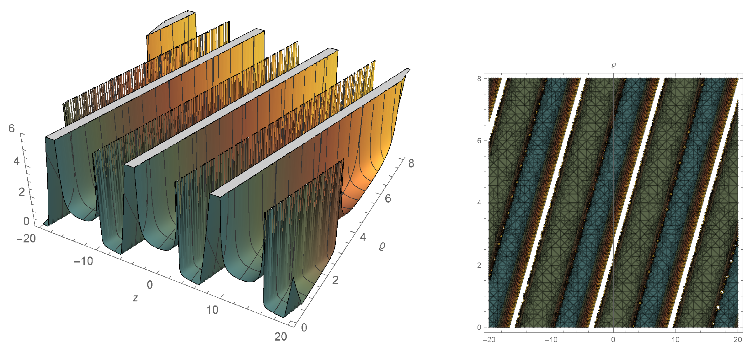
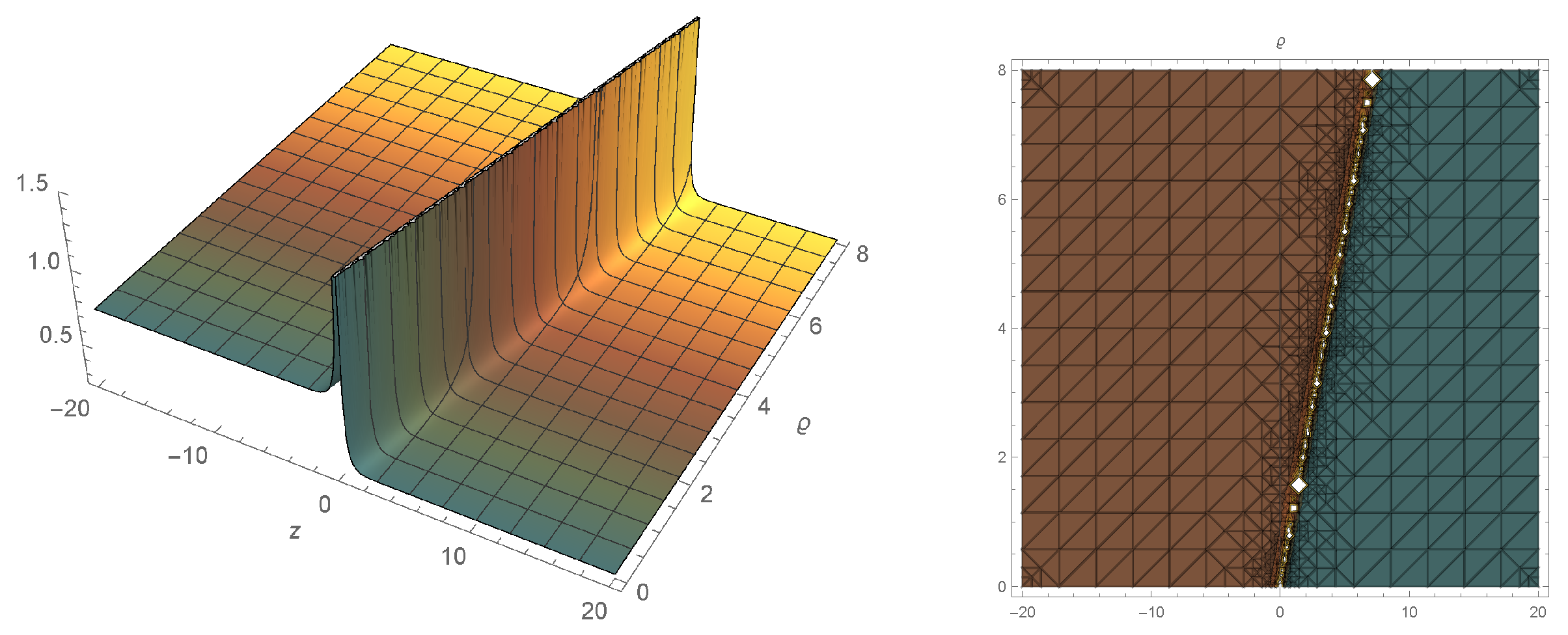
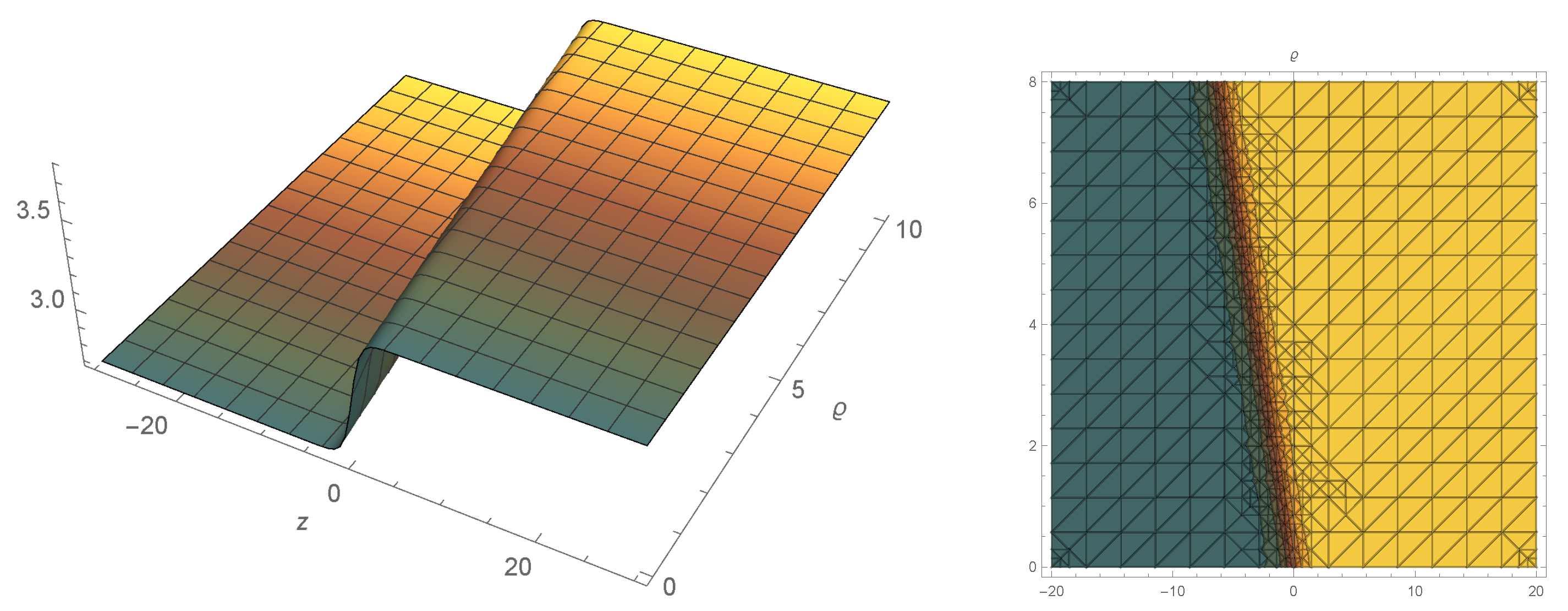
4. Graphic Representation of Solutions

In this section, 3D and contour graphs of some obtained solutions are presented to clarify the shape of some waves produced by the solutions and also to show the physical behavior of some reported solutions. Figure 1 displays a singular periodic wave solution of Equation (17) when $g_2=-0.5,G=-1.6,A=-1.6,k=0.8,\Omega =1.6,q=0.7,V=1.5$ and $-20<z<20$. Figure 2 displays a rational solution of Equation (18) when $g_2=-0.5,$$G=0.6,A=0.6,k=0.6,\Omega =0.6,q=0.7,V=0.5$ and $-10<z<15$. Figure 3 displays a singular soliton solution of Equation (19) when $g_2=-0.8,G=-1.7,A=-1.1,$$k=0.95,$$\Omega =1.6,q=1.1,V=1.7$ and $-20<z<20$. Figure 4 displays a periodic solution of Equation (24) when $g_2=1.5,G=-1.2,A=-1.4,k=1.8,\Omega =0.6,q=1.7,V=0.5$ and $-15<z<15$. Figure 5 displays a soliton solution of the bright type of Equation (27) when $g_2=2,G=-0.6,A=-0.6,k=1.1,\Omega =1.3,q=1.7,V=0.5$ and $-6<z<7$. Figure 6 displays a dark soliton solution of Equation (41) when $g_2=1.7,G=1.2,$$A=1.6,$$k=1.8,\Omega =1.6,q=-1.3,V=1.5$ and $-30<z<30$.

5. Conclusions

We investigated solitons and other solutions for the KE equation with a quintic nonlinearity and Raman effect using the improved modified extended tanh-function technique. Numerous species of solutions were obtained such as the dark soliton solutions, the bright soliton solutions, the singular soliton solution, the singular periodic solutions, the exponential solutions, the rational solutions, the Jacobi elliptic solutions, and the Weierstrass elliptic doubly periodic solutions. A graphical representation section is added to illustrate some obtained solutions.

References

1. Jagtap, A.D.; Kawaguchi, K.; Karniadakis, G.E. Adaptive activation functions accelerate convergence in deep and physics-informed neural networks. J. Comput. Phys. 2020, 404, 109136. [Google Scholar] [CrossRef] [Green Version]
2. Yin, H.M.; Pan, Q.; Chow, K.W. The Fermi–Pasta–Ulam–Tsingou recurrence for discrete systems: Cascading mechanism and machine learning for the Ablowitz–Ladik equation. Commun. Nonlinear Sci. Numer. Simul. 2022, 114, 106664. [Google Scholar] [CrossRef]
3. Zhang, R.F.; Li, M.C. Bilinear residual network method for solving the exactly explicit solutions of nonlinear evolution equations. Nonlinear Dyn. 2022, 108, 521–531. [Google Scholar] [CrossRef]
4. Alesemi, M.; Iqbal, N.; Botmart, T. Novel analysis of the fractional-order system of non-linear partial differential equations with the exponential-decay kernel. Mathematics 2022, 10, 615. [Google Scholar] [CrossRef]
5. Kudryashov, N.A. Optical solitons of the resonant nonlinear Schrödinger equation with arbitrary index. Optik 2021, 235, 166626. [Google Scholar] [CrossRef]
6. Kudryashov, N.A.; Biswas, A. Optical solitons of nonlinear Schrödinger’s equation with arbitrary dual-power law parameters. Optik 2021, 252, 168497. [Google Scholar] [CrossRef]
7. Kudryashov, N.A. Stationary solitons of the generalized nonlinear Schrödinger equation with nonlinear dispersion and arbitrary refractive index. Appl. Math. Lett. 2022, 128, 107888. [Google Scholar] [CrossRef]
8. Hu, X.; Arshad, M.; Xiao, L.; Nasreen, N.; Sarwar, A. Bright-dark and multi wave novel solitons structures of Kaup-Newell Schrödinger equations and their applications. Alex. Eng. J. 2021, 60, 3621–3630. [Google Scholar] [CrossRef]
9. Rabie, W.B.; Seadawy, A.R.; Ahmed, H.M. Highly dispersive Optical solitons to the generalized third-order nonlinear Schrödinger dynamical equation with applications. Optik 2021, 241, 167109. [Google Scholar] [CrossRef]
10. Nauman, R.N.; Hassan, Z.; Seadawy, A. Computational Soliton solutions for the variable coefficient nonlinear Schrödinger equation by collective variable method. Opt. Quantum Electron. 2021, 53, 1–16. [Google Scholar]
11. Mathanaranjan, T.; Rezazadeh, H.; Şenol, M.; Akinyemi, L. Optical singular and dark solitons to the nonlinear Schrödinger equation in magneto-optic waveguides with anti-cubic nonlinearity. Opt. Quantum Electron. 2021, 53, 1–16. [Google Scholar] [CrossRef]
12. Chen, J.; Luan, Z.; Zhou, Q.; Alzahrani, A.K.; Biswas, A.; Liu, W. Periodic soliton interactions for higher-order nonlinear Schrödinger equation in optical fibers. Nonlinear Dyn. 2020, 100, 2817–2821. [Google Scholar] [CrossRef]
13. Savaissou, N.; Gambo, B.; Rezazadeh, H.; Bekir, A.; Doka, S.Y. Exact optical solitons to the perturbed nonlinear Schrödinger equation with dual-power law of nonlinearity. Opt. Quantum Electron. 2020, 52, 1–16. [Google Scholar] [CrossRef]
14. Razzaq, W.; Zafar, A.; Ahmed, H.M.; Rabie, W.B. Construction solitons for fractional nonlinear Schrödinger equation with β-time derivative by the new sub-equation method. J. Ocean. Eng. Sci. 2022. [Google Scholar] [CrossRef]
15. Ma, G.; Zhao, J.; Zhou, Q.; Biswas, A.; Liu, W. Soliton interaction control through dispersion and nonlinear effects for the fifth-order nonlinear Schrödinger equation. NOnlinear Dyn. 2021, 106, 2479–2484. [Google Scholar] [CrossRef]
16. Liu, S.; Rezaei, S.; Najati, S.A.; Mohamed, M.S. Novel wave solutions to a generalized third-order nonlinear Schrödinger’s equation. Results Phys. 2022, 37, 105457. [Google Scholar] [CrossRef]
17. Dutta, H.; Günerhan, H.; Ali, K.K.; Yilmazer, R. Exact soliton solutions to the cubic-quartic non-linear Schrödinger equation with conformable derivative. Front. Phys. 2020, 8, 62. [Google Scholar] [CrossRef]
18. Mirzazadeh, M.; Hosseini, K.; Dehingia, K.; Salahshour, S. A second-order nonlinear Schrödinger equation with weakly nonlocal and parabolic laws and its optical solitons. Optik 2021, 242, 166911. [Google Scholar] [CrossRef]
19. Yildirim, Y. Bright, dark and singular optical solitons to Kundu–Eckhaus equation having four-wave mixing in the context of birefringent fibers by using of modified simple equation methodology. Optik 2019, 182, 110–118. [Google Scholar] [CrossRef]
20. Biswas, A.; Yildirim, Y.; Yasar, E.; Triki, H.; Alshomrani, A.S.; Ullah, M.Z.; Belic, M. Optical soliton perturbation with full nonlinearity for Kundu–Eckhaus equation by modified simple equation method. Optik 2018, 157, 1376–1380. [Google Scholar] [CrossRef] [Green Version]
21. Biswas, A.; Ekici, M.; Sonmezoglu, A.; Kara, A.H. Optical solitons and conservation law in birefringent fibers with Kundu–Eckhaus equation by extended trial function method. Optik 2019, 179, 471–478. [Google Scholar] [CrossRef]
22. El Sheikh, M.M.A.; Ahmed, H.M.; Arnous, A.H.; Rabie, W.B.; Biswas, A.; Khan, S.; Alshomrani, A.S. Optical solitons with differential group delay for coupled Kundu–Eckhaus equation using extended simplest equation approach. Optik 2020, 208, 164051. [Google Scholar] [CrossRef]
23. El-Borai, M.M.; El-Owaidy, H.M.; Hamdy, M.A.; Ahmed, H.A.; Seithuti, M.; Anjan, B.; Milivoj, B. Topological and singular soliton solution to Kundu–Eckhaus equation with extended Kudryashov’s method. Optik 2017, 128, 57–62. [Google Scholar] [CrossRef]
24. Triki, H.; Sun, Y.; Biswas, A.; Zhou, Q.; Yıldırım, Y.; Zhong, Y.; Alshehri, H.M. On the existence of chirped algebraic solitary waves in optical fibers governed by Kundu–Eckhaus equation. Results Phys. 2022, 34, 105272. [Google Scholar] [CrossRef]
25. Yang, Z.; Hon, B.Y. An improved modified extended tanh-function method. Z. Naturforschung A 2006, 61, 103–115. [Google Scholar] [CrossRef]
26. Esen, H.; Ozisik, M.; Secer, A.; Bayram, M. Optical soliton perturbation with Fokas–Lenells equation via enhanced modified extended tanh-expansion approach. Optik 2022, 267, 169615. [Google Scholar] [CrossRef]
Figure 1. Three-dimensional (3D) and contour plots of the singular periodic wave solution of Equation (17).
Mathematics 10 04203 g001
Figure 2. Three-dimensional (3D) and contour plots of the rational solution of Equation (18).
Mathematics 10 04203 g002
Figure 3. Three-dimensional (3D) and contour plots of the singular soliton solution of Equation (19).
Mathematics 10 04203 g003
Figure 4. Three-dimensional (3D) and contour plots of the periodic solution of Equation (24).
Mathematics 10 04203 g004
Figure 5. Three-dimensional (3D) and contour plots of the bright soliton solution of Equation (27).
Mathematics 10 04203 g005
Figure 6. Three-dimensional (3D) and contour plots of the dark soliton solution of Equation (41).
Mathematics 10 04203 g006
Publisher’s Note: MDPI stays neutral with regard to jurisdictional claims in published maps and institutional affiliations.