The Analytical Solutions of the Stochastic mKdV Equation via the Mapping Method

Abstract

Here, we analyze the (2+1)-dimensional stochastic modified Kordeweg–de Vries (SmKdV) equation perturbed by multiplicative white noise in the Stratonovich sense. We apply the mapping method to obtain new trigonometric, elliptic, and rational stochastic fractional solutions. Because of the importance of the KdV equation in characterizing the behavior of waves in shallow water, the obtained solutions are beneficial in interpreting certain fascinating physical phenomena. We plot our figures in MATLAB and show several 3D and 2D graphical representations to show how the multiplicative white noise affects the solutions of the SmKdV. We show that the white noise around zero stabilizes SmKdV solutions.

1. Introduction

The development of innovative traveling wave solutions for non-linear partial differential equations (NLPDEs) is crucial and important from many viewpoints for the most physical mathematical phenomena.The non-linear wave phenomenon occurs in a variety of disciplines of science and engineering, including meteorology, geology, solid-state physics, biology, chemical kinematics, fluid-mechanics, ocean engineering, and chemical physics [1,2,3,4]. In non-linear wave equations, the non-linear wave phenomena of convection, diffusion, dispersion, response, and dissipation are very significant. Consequently, one of the central issues of interest in physics and mathematics has been the study of exact solutions to those equations. Numerous techniques, such as the generalized Kudryashov method [5], sine-Gordon expansion [6,7], Exp-function [8], perturbation [9,10], Lie symmetry [11], Ricatti equation expansion [12], sn-ns method [13], Bernoulli sub-equation function [14], improved $tan(\phi /2)$-expansion [15], tanh-sech [16,17,18], and ($G^{\prime }/G$)-expansion [19], have been explored, and some of them have been created in the process of looking for exact solutions to those equations.

One of the most familiar models for NLPDEs is the Korteweg–de Vries (KdV) equation:

$${\phi }_t+6\phi {\phi }_x+{\phi }_{xxx}=0.$$

(1)

The KdV equation explains ion acoustic-waves in plasma, acoustic-waves on a crystal lattice, and long internal waves in a density-stratified ocean and in weakly interacting shallow-water waves. Numerous researchers have explored various forms of the KdV equation using different methodologies and approaches from a variety of perspectives (see, for example, Refs. [20,21,22,23,24,25,26,27] and the references therein).

On the other hand, the modified Kordeweg–de Vries (mKdV) equation

$${\phi }_t+6{\phi }^2{\phi }_x+{\phi }_{xxx}=0,$$

(2)

has had a significant impact on the history of soliton theory. Additionally, it was employed to create an unlimited number of conservation laws for the KdV equation [28], that led to the identification of the Lax pair for the KdV equation and the invention of the inverse scattering transform [29]. Many authors have addressed exact solutions using different methods, such as the Exp-function [30], first integral [31], ($G^{\prime }/G$)-expansion [32], and tanh methods [33], Bifurcation [34], etc.

A new (2+1)-dimensional mKdV equation that depends on the extended Lax equation was established and reported in 2019 [35] in the following form

$${\phi }_t+6{\phi }^2({\phi }_y-{\phi }_x)-{\phi }_{xxx}+{\phi }_{yyy}+3{\phi }_{xxy}-3{\phi }_{xyy}=0.$$

(3)

It is worth noting that if $\phi$ does not rely on x, i.e., $\phi =\phi (y,t)$, then Equation (3) turns out the mKdV equation

$${\phi }_t+6{\phi }^2{\phi }_y+{\phi }_{yyy}=0.$$

(4)

If we rewrite the variable y as x, we have the mKdV Equation (2). The mKdV equation has multiple uses, including fluid mechanics [36], the dynamics of traffic flow [37], and the study of waves propagating in plasma [38]. Additionally, it is utilized in non-linear optics to explain pulses made up of a few optical cycles [39].

In recent years, the realization of adding random effects when predicting, modeling, simulating, and evaluating complex systems has been extensively appreciated in telecommunications, cryptography, biology, computer science, signal processing, climatic dynamics, physics, chemistry, geophysics, neuroscience, ecology, and other domains. Therefore, here, we consider Equation (3), which is derived by multiplicative noise, in the following form:

$$d\phi +[6{\phi }^2({\phi }_y-{\phi }_x)-{\phi }_{xxx}+{\phi }_{yyy}+3{\phi }_{xxy}-3{\phi }_{xyy}]dt=\sigma \phi \circ d\beta .$$

(5)

where $\beta \left(t\right)$ is the white noise and $\sigma$ is the intensity of noise.

If we evaluate the stochastic integral in the middle, the integral ${\int }_0^t\phi \left(\tau \right)d\beta \left(\tau \right)$ is called the Stratonovich stochastic integral (denoted by ${\int }_0^t\phi \left(\tau \right)\circ d\beta \left(\tau \right)$). If we evaluate it at the left end, the integral ${\int }_0^t\phi \left(\tau \right)d\beta \left(\tau \right)$ is called the Itô stochastic integral (denoted by ${\int }_0^t\phi \left(\tau \right)d\beta \left(\tau \right)$) [40]. The Itô integral and Stratonovich integral have the following relationship:

$${\int }_0^t\sigma \phi \left(\tau \right)d\beta \left(\tau \right)={\int }_0^t\sigma \phi \left(\tau \right)\circ d\beta \left(\tau \right)-\frac{{\sigma }^2}{2}{\int }_0^t\phi \left(\tau \right)d\tau .$$

(6)

Our objective is to apply the mapping method to determine the exact stochastic solutions of the SmKdV Equation (5). The solutions provided would be tremendously helpful to physicists in characterizing some important physical phenomena. Additionally, we explore the influence of noise on the analytical solutions of the SmKdV Equation (5) by introducing several figures through the use of MATLAB software.

The following is the order of the article: In Section 2, we employ wave transformation to attain the wave equation for the stochastic SmKdV Equation (5). In Section 3, we describe the mapping method, which we use in this article. In Section 4, the mapping method is used to ensure the exact stochastic solution of the SmKdV Equation (5). Next, in Section 5, we can see the influence of white noise on the acquired solutions of the SmKdV equation. Finally, the article’s conclusions are provided.

2. Traveling Wave Equation for SmKdV

The wave equation for the SmKdV Equation (5) is obtained using the transformation:

$$\phi (x,y,t)=\psi \left(\mu \right)e^{[\sigma \beta \left(t\right)-{\sigma }^{2}t]},\mu ={\mu }_{1}x+{\mu }_{2}y+{\mu }_{3}t,$$

(7)

where $\psi$ is a real deterministic function and ${\mu }_1,{\mu }_2,{\mu }_3$ are non-zero constants. We note that

$$\begin{array}{ccc}\hfill d\phi & =& [{\mu }_3{\psi }^{\prime }dt+\sigma \psi d\beta -\frac{1}{2}{\sigma }^2\psi dt]e^{[\sigma \beta \left(t\right)-{\sigma }^{2}t]}\hfill \\ & =& [{\mu }_3{\psi }^{\prime }dt+\sigma \psi \circ d\beta ]e^{[\sigma \beta \left(t\right)-{\sigma }^{2}t]},\hfill \end{array}$$

(8)

and

$$\begin{array}{ccc}\hfill {\phi }_x& =& {\mu }_1{\psi }^{\prime }{e}^{[\sigma \beta \left(t\right)-{\sigma }^{2}t]},{\phi }_{xxx}={\mu }_1^3{\psi }^{‴}{e}^{[\sigma \beta \left(t\right)-{\sigma }^{2}t]},\hfill \\ \hfill {\phi }_y& =& {\mu }_2{\psi }^{\prime }{e}^{[\sigma \beta \left(t\right)-{\sigma }^{2}t]},{\phi }_{yyy}={\mu }_2^3{\psi }^{‴}{e}^{[\sigma \beta \left(t\right)-{\sigma }^{2}t]}\hfill \\ \hfill {\phi }_{xxy}& =& {\mu }_1^2{\mu }_2{\psi }^{‴}{e}^{[\sigma \beta \left(t\right)-{\sigma }^{2}t]},{\phi }_{xyy}={\mu }_1{\mu }_2^2{\psi }^{‴}{e}^{[\sigma \beta \left(t\right)-{\sigma }^{2}t]}.\hfill \end{array}$$

(9)

Inserting Equation (7) into (5) and utilizing (8) and (9), we obtain

$${({\mu }_2-{\mu }_1)}^3{\psi }^{‴}+{\mu }_3{\psi }^{\prime }+6({\mu }_2-{\mu }_1){\psi }^2{\psi }^{\prime }{e}^{[2\sigma \beta \left(t\right)-2{\sigma }^{2}t]}=0.$$

(10)

Considering the expectations on both sides, we attain

$${({\mu }_2-{\mu }_1)}^3{\psi }^{‴}+{\mu }_3{\psi }^{\prime }+6({\mu }_2-{\mu }_1){\psi }^2{\psi }^{\prime }{e}^{-2{\sigma }^{2}t}\mathbb{E}{e}^{\left[2\sigma \beta \right(t\left)\right]}=0.$$

(11)

Since $\beta \left(t\right)$ is the normal process, then $E\left(e^{2\sigma \beta \left(t\right)}\right)=e^{2{\sigma }^{2}t}$. Therefore, Equation (11) becomes

$${({\mu }_2-{\mu }_1)}^3{\psi }^{‴}+{\mu }_3{\psi }^{\prime }+6({\mu }_2-{\mu }_1){\psi }^2{\psi }^{\prime }=0.$$

(12)

Integrating Equation (12) once and setting the constant of integration equal to zero, we have the following Duffing equation

$${\psi }^{″}+{\ell }_1{\psi }^3+{\ell }_2\psi =0,$$

(13)

where

$${\ell }_1=\frac{2}{{({\mu }_2-{\mu }_1)}^2}\mathrm{and}{\ell }_2=\frac{{\mu }_3}{{({\mu }_2-{\mu }_1)}^3}.$$

3. The Description of Mapping Method

Let us now explain the mapping method stated in Ref. [41]. Supposing that the solutions to Equation (13) are

$$\psi \left(\mu \right)=\sum _{i=0}^m{\hslash }_i{F}^i\left(\mu \right),$$

(14)

where ${\hslash }_i,$ for $i=1,2,\dots ,{\hslash }_m,$ are undefined constants to be evaluated and F fulfills the first type of elliptic equation

$$F^{\prime }=\sqrt{r+q{F}^2+p{F}^4},$$

(15)

where the parameters r, q, and p are real.

We see that Equation (15) has several solutions based on $r,q$, and p as following

Table 1. All solutions for Equation (15) for various $r,q$, and p values.

Case	p	q	r	$\mathit{F}\left(\mathit{\mu }\right)$
1	${\kappa }^2$	$-(1+{\kappa }^2)$	1	$sn\left(\mu \right)$
2	1	$2{\kappa }^2-1$	$-{\kappa }^2(1-{\kappa }^2)$	$ds\left(\mu \right)$
3	1	$2-{\kappa }^2$	$(1-{\kappa }^2)$	$cs\left(\mu \right)$
4	$-{\kappa }^2$	$2{\kappa }^2-1$	$(1-{\kappa }^2)$	$cn\left(\mu \right)$
5	$-1$	$2-{\kappa }^2$	$({\kappa }^2-1)$	$dn\left(\mu \right)$
6	$\frac{{\kappa }^2}{4}$	$\frac{({\kappa }^2-2)}{2}$	$\frac{1}{4}$	$\frac{sn\left(\mu \right)}{1\pm dn\left(\mu \right)}$
7	$\frac{{\kappa }^2}{4}$	$\frac{({\kappa }^2-2)}{2}$	$\frac{{\kappa }^2}{4}$	$\frac{sn\left(\mu \right)}{1\pm dn\left(\mu \right)}$
8	$\frac{-1}{4}$	$\frac{({\kappa }^2+1)}{2}$	$\frac{-{(1-{\kappa }^2)}^2}{4}$	$\kappa cn\left(\mu \right)\pm dn\left(\mu \right)$
9	$\frac{{\kappa }^2-1}{4}$	$\frac{({\kappa }^2+1)}{2}$	$\frac{({\kappa }^2-1)}{4}$	$\frac{dn\left(\mu \right)}{1\pm sn\left(\mu \right)}$
10	$\frac{1-{\kappa }^2}{4}$	$\frac{(1-{\kappa }^2)}{2}$	$\frac{(1-{\kappa }^2)}{4}$	$\frac{cn\left(\mu \right)}{1\pm sn\left(\mu \right)}$
11	$\frac{{(1-{\kappa }^2)}^2}{4}$	$\frac{{(1-{\kappa }^2)}^2}{2}$	$\frac{1}{4}$	$\frac{sn\left(\mu \right)}{dn\pm cn\left(\mu \right)}$
12	1	0	0	$\frac{c}{\mu }$
13	0	1	0	$c{e}^{\mu }$

:

Where $cn\left(\mu \right)=cn(\mu ,\kappa ),sn\left(\mu \right)=sn(\mu ,\kappa ),dn\left(\mu \right)=dn(\mu ,\kappa )$, for $0<\kappa <1$ are the Jacobi elliptic functions (JEFs). If $\kappa \to$ 1, then JEFs are transformed into the following hyperbolic functions:

$$\begin{array}{ccc}\hfill cs\left(\mu \right)& \to & csch\left(\mu \right),sn\left(\mu \right)\to tanh\left(\mu \right),cn\left(\mu \right)\to sech\left(\mu \right),\hfill \\ \hfill dn\left(\mu \right)& \to & sech\left(\mu \right),ds\to csch\left(\mu \right).\hfill \end{array}$$

4. Exact Solutions of mKdV

To find the parameter m, let us equalize ${\psi }^{″}$ with ${\psi }^3$ in Equation (13) as

$$m+2=3m⟹m=1.$$

Rewriting Equation (15) with $m=1$ as

$$\psi \left(\mu \right)={\hslash }_0+{\hslash }_{1}F\left(\mu \right).$$

(16)

Differentiating Equation (16) twice and using (15), we obtain

$${\psi }^{″}={\hslash }_{1}qF+{\hslash }_{1}p{F}^3.$$

(17)

Plugging Equations (16) and (17) into Equation (13) we have

$$({\hslash }_{1}p+{\ell }_1{\hslash }_1^3)F^3+3{\hslash }_0{\hslash }_1^2{\ell }_1{F}^2+({\hslash }_{1}q+3{\ell }_1{\hslash }_0^2{\hslash }_1+{\ell }_2{\hslash }_1)F+({\ell }_1{\hslash }_0^3+{\ell }_2{\hslash }_0)=0.$$

Comparing each coefficient of $F^j$ with zero, we attain

$${\hslash }_{1}p+{\ell }_1{\hslash }_1^3=0,$$

$$3{\hslash }_0{\hslash }_1^2{\ell }_1=0,$$

$${\hslash }_{1}q+3{\ell }_1{\hslash }_0^2{\hslash }_1+{\ell }_2{\hslash }_1=0,$$

and

$${\ell }_1{\hslash }_0^3+{\ell }_2{\hslash }_0=0.$$

When we solve these equations, we obtain

$${\hslash }_0=0,{\hslash }_1=\pm \sqrt{\frac{-p}{{\ell }_1}},q=-{\ell }_2.$$

Therefore, Equation (13) has the solution:

$$\psi \left(\mu \right)=\pm \sqrt{\frac{-p}{{\ell }_1}}F\left(\mu \right),$$

(18)

for $p<0$ where ${\ell }_1=\frac{2}{{({\mu }_2-{\mu }_1)}^2}>0.$ There are many cases for the solutions $\psi \left(\mu \right)$ of Equation (13) relying on p as shown in Table 1, as following

Table 2. All solutions for wave Equation (13) when $p<0$.

Case	p	q	r	$\mathit{F}\left(\mathit{\mu }\right)$	$\mathit{\psi }\left(\mathit{\mu }\right)$
1	$-{\kappa }^2$	$2{\kappa }^2-1$	$(1-{\kappa }^2)$	$cn\left(\mu \right)$	$\pm \sqrt{\frac{-p}{{\ell }_1}}cn\left(\mu \right)$
2	$-1$	$2-{\kappa }^2$	$({\kappa }^2-1)$	$dn\left(\mu \right)$	$\pm \sqrt{\frac{-p}{{\ell }_1}}dn\left(\mu \right)$
3	$\frac{-1}{4}$	$\frac{({\kappa }^2+1)}{2}$	$\frac{-{(1-{\kappa }^2)}^2}{4}$	$\kappa cn\left(\mu \right)\pm dn\left(\mu \right)$	$\pm \sqrt{\frac{-p}{{\ell }_1}}[\kappa cn\left(\mu \right)\pm dn\left(\mu \right)]$
4	$\frac{{\kappa }^2-1}{4}$	$\frac{({\kappa }^2+1)}{2}$	$\frac{({\kappa }^2-1)}{4}$	$\frac{dn\left(\mu \right)}{1\pm sn\left(\mu \right)}$	$\pm \sqrt{\frac{-p}{{\ell }_1}}\frac{dn\left(\mu \right)}{1\pm sn\left(\mu \right)}$

:

If $\kappa \to 1$, then Table 2 degenerates to

Table 3. All solutions for wave Equation (13) when $\kappa \to 1$ and $p<0$.

Case	p	q	r	$\mathit{F}\left(\mathit{\mu }\right)$	$\mathit{\psi }\left(\mathit{\mu }\right)$
1	$-1$	1	0	$sech\left(\mu \right)$	$\pm \sqrt{\frac{1}{{\ell }_1}}sech\left(\mu \right)$
2	$\frac{-1}{4}$	2	0	$2sech\left(\mu \right)$	$\pm \sqrt{\frac{1}{{\ell }_1}}sech\left(\mu \right)$

.

Now, by utilizing Table 2 (or Table 3 when $\kappa \to 1$), we can have the exact solutions of the SmKdV Equation (5) as follows:

$$\phi (x,y,t)=\psi \left(\mu \right)e^{[\sigma \beta \left(t\right)-{\sigma }^{2}t]}.$$

(19)

Remark 1. 

We can use various methods, including the Adomian decomposition, $exp(-\phi )$-expansion method, improved $tan\left(\frac{\varphi \left(\rho \right)}{2}\right)$ expansion, extended tanh method, Exp-function, Hirota bilinear, Weierstrass elliptic function, extended trial equation, complex hyperbolic function, etc., to obtain various solutions.

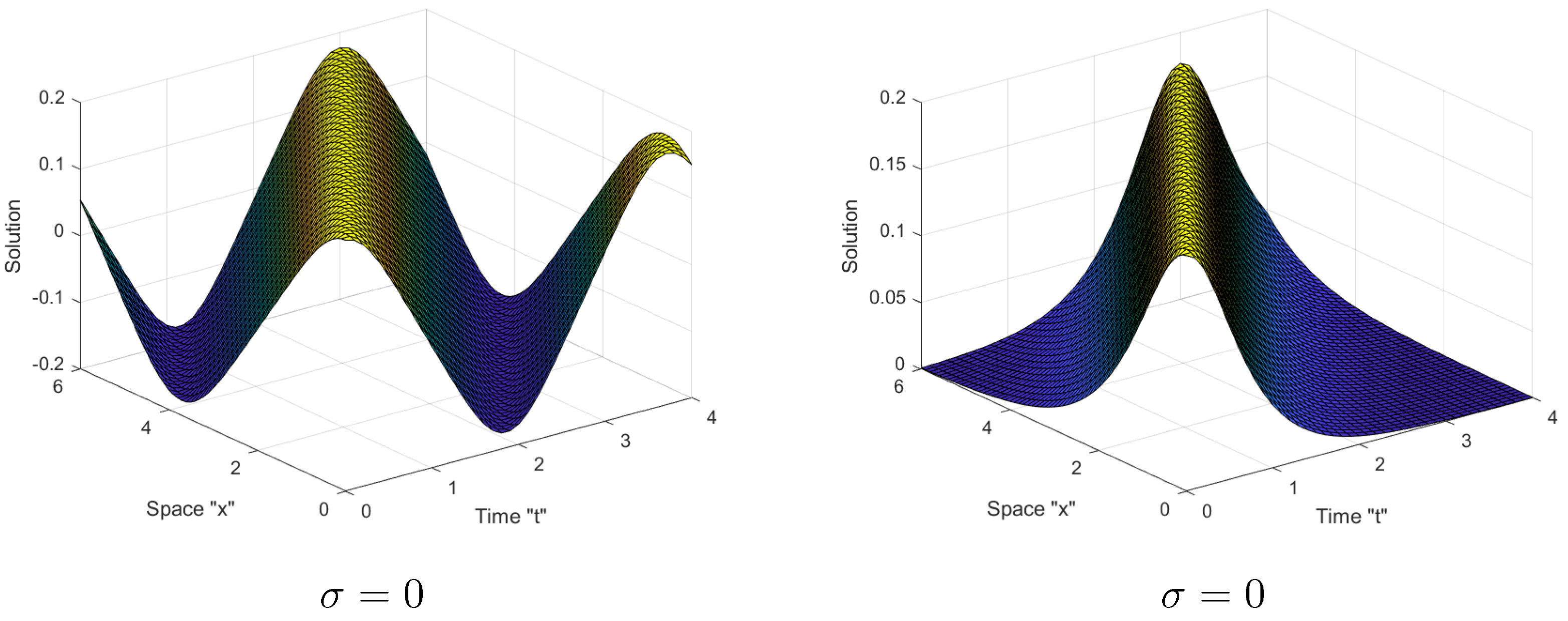
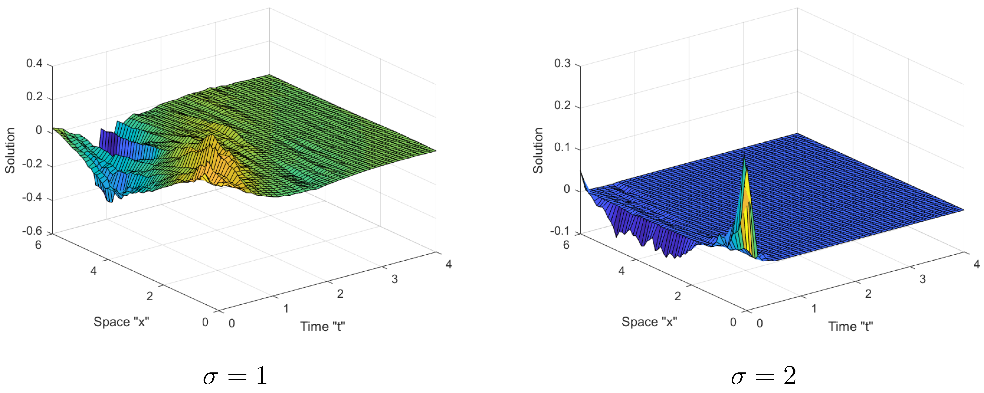
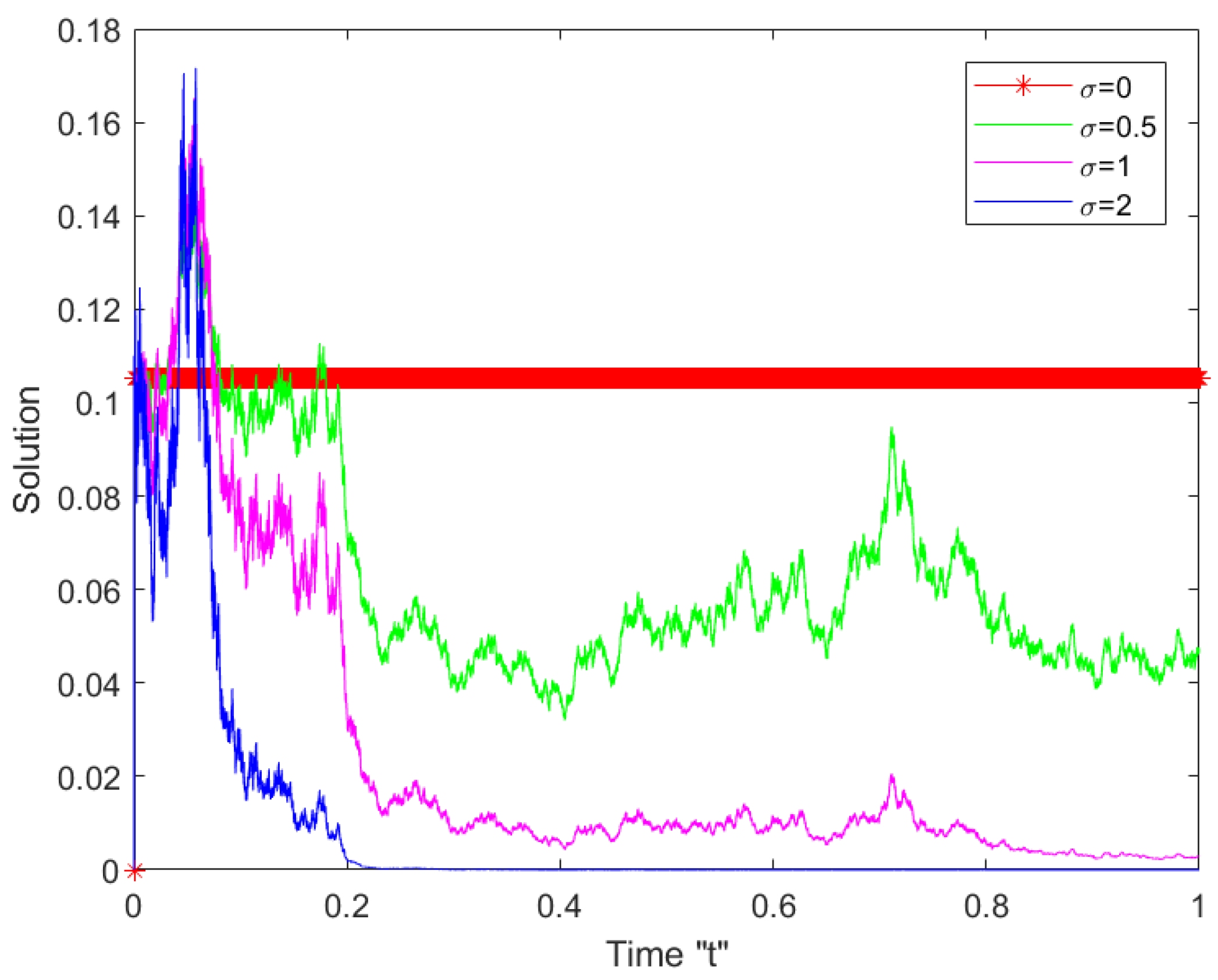
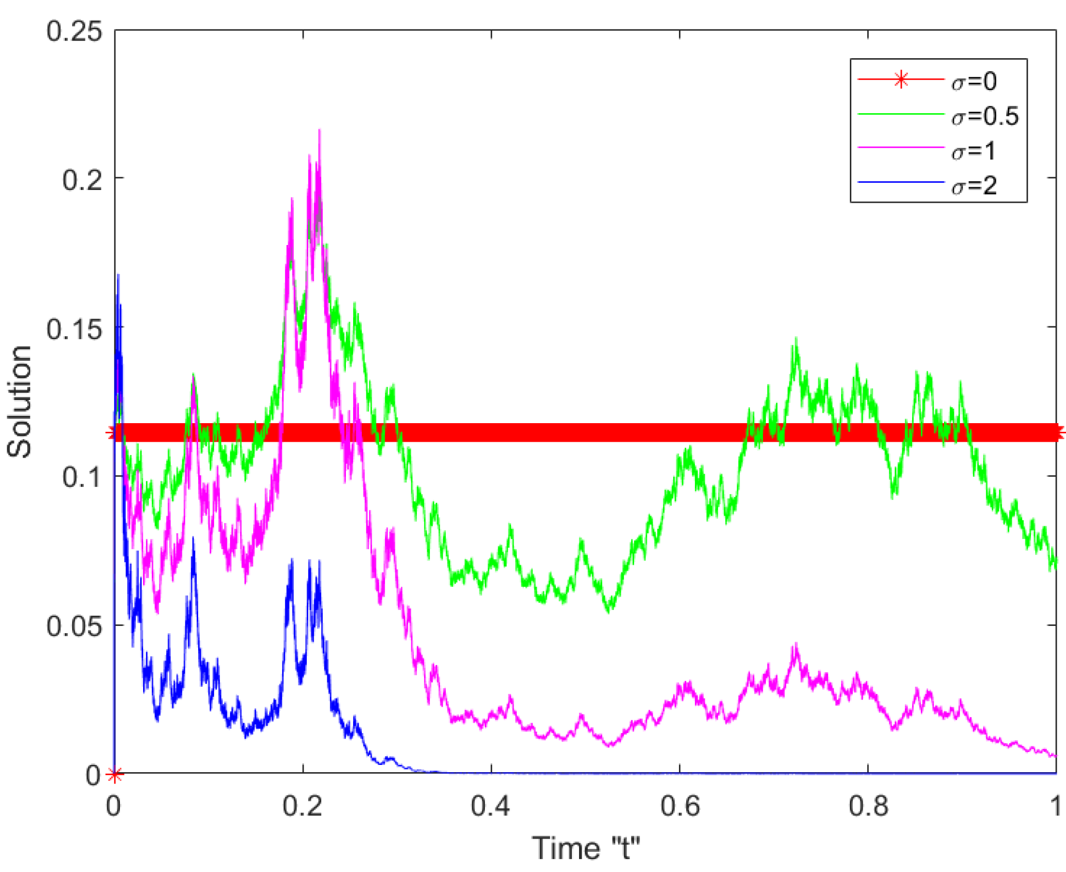
5. The Effect of Noise on SmKdV Solutions

Here, we address the effect of white noise on the analytical solutions of the SmKdV Equation (5). We give various figures to describe the behavior of these solutions. For various $\sigma$ (noise strength), we simulate some figures for obtained solutions, such as

$$\phi (x,y,t)=\frac{\kappa }{\sqrt{2}}\left|{\mu }_2-{\mu }_1\right|cn({\mu }_{1}x+{\mu }_{2}y+{\mu }_{3}t)e^{[\sigma \beta \left(t\right)-{\sigma }^{2}t]},$$

(20)

and

$$\phi (x,y,t)=\frac{1}{\sqrt{2}}\left|{\mu }_2-{\mu }_1\right|sech({\mu }_{1}x+{\mu }_{2}y+{\mu }_{3}t)e^{[\sigma \beta \left(t\right)-{\sigma }^{2}t]}.$$

(21)

Let us first fix the parameters ${\mu }_1, {\mu }_2$, and ${\mu }_3$ as follows: ${\mu }_1=1,{\mu }_2=0.5,$ ${\mu }_3=-2$, and $\kappa =0.5.$ Additionally, let $y=0,x\in [0,5]$ and $t\in [0,5].$ In the next Figure 1, when there is no noise (i.e., $\sigma =0$), we observe that the surface fluctuates

While we see that in Figure 2 and Figure 3, after minor transit behaviors, the surface turn into more planar:

In Figure 4 and Figure 5, we draw a two-dimensional graph representing the solution $\phi (x,y,t)$ in Equations (20) and (21) to illustrate our previous results as follows:

6. Conclusions

In this paper, we took into account the stochastic mKdV equation, which was created in the Stratonovich sense by multiplicative white noise. Utilizing the mapping method, we were able to obtain exact solutions. These solutions play a vital role in describing a number of interesting and complicated physical phenomena. Finally, the MATLAB package was used to demonstrate the effect of multiplicative white noise on the exact solution of the SmKdV equation.

References

1. Johnson, R.S. Anon-linear equation incorporating damping and dispersion. J. Fluid Mech. 1970, 42, 49–60. [Google Scholar] [CrossRef]
2. Younis, M.; Ali, S. Solitary wave and shock wave solutions to the transmission line modelfor nano-ionic currents along microtubules. Appl. Math. Comput. 2014, 246, 460–463. [Google Scholar]
3. Younis, M.; Rizvi, S.T.R.; Ali, S. Analytical and soliton solutions: Nonlinear model of nanobioelectronics transmis sion lines. Appl. Math. Comput. 2015, 265, 994–1002. [Google Scholar] [CrossRef]
4. Razborova, P.; Moraru, L.; Biswas, A. Perturbation of dis persive shallow water waves with Rosenau- KdV RLW equation and power law nonlinearity. Rom. J. Phys. 2014, 59, 7–8. [Google Scholar]
5. Zhou, Q.; Ekici, M.; Sonmezoglu, A.; Manafian, J.; Khaleghizadeh, S.; Mirzazadeh, M. Exact solitary wave solutions to the generalized Fisher equation. Optik 2016, 127, 12085–12092. [Google Scholar] [CrossRef]
6. Baskonus, H.M.; Bulut, H. New wave behaviors of the system of equations for the ion sound and Langmuir Waves. Waves Random Complex Media 2016, 26, 613–625. [Google Scholar] [CrossRef]
7. Baskonus, H.M. New acoustic wave behaviors to the Davey-Stewartson equation with power-law nonlinearity arising in fluid dynamics. Nonlinear Dyn. 2016, 86, 177–183. [Google Scholar] [CrossRef]
8. Manafian, J.; Lakestani, M. Optical solitons with Biswas-Milovic equation for Kerr law nonlinearity. Eur. Phys. J. Plus 2015, 130, 61. [Google Scholar] [CrossRef]
9. Mohammed, W.W.; Blömker, D. Fast-diffusion limit for reaction-diffusion equations with multiplicative noise. J. Math. Anal. Appl. 2021, 496, 124808. [Google Scholar] [CrossRef]
10. Mohammed, W.W.; Iqbal, N. Impact of the same degenerate additive noise on a coupled system of fractional space diffusion equations. Fractals 2022, 30, 2240033. [Google Scholar] [CrossRef]
11. Tchier, F.; Yusuf, A.; Aliyu, A.I.; Inc, M. Soliton solutions and conservation laws for lossy nonlinear transmission line equation. Superlattices Microstruct. 2017, 107, 320–336. [Google Scholar] [CrossRef]
12. Zhou, Q. Optical solitons in medium with parabolic law nonlinearity and higher order dispersion. Waves Random Complex Media 2016, 25, 52–59. [Google Scholar] [CrossRef]
13. Salas, A.H. Solving nonlinear partial differential equations by the sn-ns method. Abstr. Appl. Anal. 2012, 2012, 340824. [Google Scholar] [CrossRef] [Green Version]
14. Baskonus, H.M.; Bulut, H. Exponential prototype structures for (2+1)-dimensional Boiti-Leon-Pempinelli systems in mathematical physics. Waves Random Complex Media 2016, 26, 201–208. [Google Scholar] [CrossRef]
15. Manafian, J. Optical soliton solutions for Schrodinger type nonlinear evolution equations by the tan(φ/2)-expansion method. Optik 2016, 127, 4222–4245. [Google Scholar] [CrossRef]
16. Wazwaz, A.M. The tanh method: Exact solutions of the Sine–Gordon and Sinh–Gordon equations. Appl. Math. Comput. 2005, 167, 1196–1210. [Google Scholar] [CrossRef]
17. Mohammed, W.W.; Alshammari, M.; Cesarano, C.; El-Morshedy, M. Brownian Motion Effects on the Stabilization of Stochastic Solutions to Fractional Diffusion Equations with Polynomials. Mathematics 2022, 10, 1458. [Google Scholar] [CrossRef]
18. Al-Askar, E.M.; Mohammed, W.W.; Albalahi, A.M.; El-Morshedy, M. The Impact of the Wiener process on the analytical solutions of the stochastic (2+1)-dimensional breaking soliton equation by using tanh–coth method. Mathematics 2022, 10, 817. [Google Scholar] [CrossRef]
19. Manafian, J.; Lakestani, M. Solitary wave and periodic wave solutions for Burgers, Fisher, Huxley and combined forms of these equations by the (G′/G)-expansion method. Pramana J. Phys. 2015, 130, 31–52. [Google Scholar] [CrossRef]
20. Ablowitz, M.J.; Segur, H. Solitons and the Inverse Scattering Transform; SIAM: Philadelphia, PA, USA, 1981. [Google Scholar]
21. Hirota, R. The Direct Method in Soliton Theory; Osaka City University: Osaka, Japan, 2004. [Google Scholar]
22. Olver, P.J. Application of Lie Group to Differential Equation; Springer: New York, NY, USA, 1986. [Google Scholar]
23. Wazwaz, A.M. A KdV6 hierarchy: Integrable members with distinct dispersion relations. Appl. Math. Lett. 2015, 45, 86–92. [Google Scholar] [CrossRef]
24. Geng, X.; Xue, B. N-soliton and quasi-periodic solutions of the KdV6 equations. Appl. Math. Comp. 2012, 219, 3504–3510. [Google Scholar] [CrossRef]
25. Azwaz, A.M.; Xu, G.Q. An extended modified KdV equation and its Painlevé integrability. Nonlinear Dyn. 2016, 86, 1455–1460. [Google Scholar] [CrossRef]
26. Zhang, Y.; Dang, X.L.; Xu, H.X. Backlund transformations and soliton solutions for the KdV6 equation. Appl. Math. Comp. 2011, 217, 6230–6236. [Google Scholar] [CrossRef]
27. Wen, X.Y.; Gao, Y.T.; Wang, L. Darboux transformation and explicit solutions for the integrable sixth-order KdV equation for nonlinear waves. Appl. Math. Comp. 2011, 218, 55–60. [Google Scholar] [CrossRef]
28. Miura, R.M.; Gardner, C.S.; Kruskal, M.D. KdV equation and generalizations.II. Existence of conservation laws and constant of motion. J. Math. Phys. 1968, 9, 1204–1209. [Google Scholar] [CrossRef]
29. Gardner, C.S.; Green, J.M.; Kruskal, M.D.; Miura, R.M. Method for solving the Korteweg–de Vries equation. Phys. Rev. Lett. 1967, 19, 1095–1097. [Google Scholar] [CrossRef]
30. Raslan, K.R. The application of He’s Exp-function method for MKdV and Burgers’ equations with variable coefficients. Int. Nonlinear Sci. 2009, 7, 174–181. [Google Scholar]
31. Yang, Y. Exact solutions of the mKdV equation. IOP Conf. Ser. Earth Environ. Sci. 2021, 769, 042040. [Google Scholar] [CrossRef]
32. Taghizadeh, N. Comparison of solutions of mKdV equation by using the first integral method and (G′/G)-expansion method. Math. Aeterna 2012, 2, 309–320. [Google Scholar]
33. Wazwaz, A.M. The tanh method for generalized forms of nonlinear heat conduction and Burgers–Fisher equations. Appl. Math. Comput. 2005, 169, 321–338. [Google Scholar] [CrossRef]
34. Elmandouha, A.A.; Ibrahim, A.G. Bifurcation and travelling wave solutions for a (2+1)-dimensional KdV equation. J. Taibah Univ. Sci. 2020, 14, 139–147. [Google Scholar] [CrossRef] [Green Version]
35. Wang, G.; Kara, A.H. A (2+1)-dimensional KdV equation and mKdV equation: Symmetries, group invariant solu tions and conservation laws. Phys. Lett. A 2019, 383, 728–731. [Google Scholar] [CrossRef]
36. Helal, M.A. Soliton solution of some nonlinear partial differential equations and its applications in fluid mechanics. Chaos Solitons Fractals 2002, 13, 1917–1929. [Google Scholar] [CrossRef]
37. Li, Z.P.; Liu, Y.C. Analysis of stability and density waves of traffic flow model in an ITS environment. Eur. Phys. J. B 2006, 53, 367–374. [Google Scholar] [CrossRef]
38. Khater, A.H.; El-Kalaawy, O.H.; Callebaut, D.K. Bäcklund transformations and exact solutions for Alfven solitons in a relativistic electronpositron plasma. Phys. Scr. 1998, 58, 545–548. [Google Scholar] [CrossRef]
39. Leblond, H.; Mihalache, D. Few-optical-cycle solitons: Modified Kortewegde Vries sine-Gordon equation versus other non-slowly-varying-envelopeapproximation models. Phys. Rev. A 2009, 79, 063835-1-7. [Google Scholar] [CrossRef] [Green Version]
40. Kloeden, P.E.; Platen, E. Numerical Solution of Stochastic Differential Equations; Springer: New York, NY, USA, 1995. [Google Scholar]
41. Peng, Y.Z. Exact solutions for some nonlinear partial differential equations. Phys. Lett. A 2013, 314, 401–408. [Google Scholar] [CrossRef]
Figure 1. 3D-diagram of solution φ ( x , y , t ) in Equations (20) and (21).
Mathematics 10 04212 g001
Figure 2. 3D-diagram of solution φ ( x , y , t ) in Equation (20) for different σ = 1 , 2 .
Mathematics 10 04212 g002
Figure 3. 3D-diagram of solution φ ( x , y , t ) in Equation (21) for different σ = 1 , 2 .
Mathematics 10 04212 g003
Figure 4. 2D-diagram of solution φ ( x , y , t ) in Equation (20).
Mathematics 10 04212 g004
Figure 5. 2D-diagram of solution φ ( x , y , t ) in Equation (21).
Mathematics 10 04212 g005