1. Introduction
Parkinson’s disease (PD) is the second most common age-related neurodegenerative disease only after Alzheimer’s disease. It occurs when people get older. It affects their nervous system, causing them to tremble and stiffen, and resulting in difficulty in walking, standing, and organizing their actions [
1]. It also has an impact on the voice and causes other cognitive issues. Both motor and non-motor signs are present in Parkinson’s disease. Motor symptoms include tremors, slowness of movement due to muscle stiffness, gait issues, and speech difficulties. Non-motor symptoms, on the other hand, include sleep, mood, and cognitive disorders, such as memory loss, sleep difficulties, and impaired abstract thought, problem-solving, vocabulary, and visual emotional capacities. The disease is caused by the degeneration of a brain area called the “substantia nigra” in the thalamic region. The dopamine hormone, a synaptic information-relaying neurotransmitter, is in charge of brain and body coordination. PD is characterized by a decrease in dopamine hormone production, which impairs brain–body coordination.
Because there is no treatment for Parkinson’s disease unless it is discovered early, numerous researchers have been working in this sector for the past few years to develop a method for early detection. Utilizing the PD dataset from the University of California-Irvine’s (UCI) deep learning database of speech signals, M. Hariharan et al. developed a hybrid approach for identifying PD using three supervised classifiers. Least squares support vector machines, probabilistic neural networks, and general regression neural networks were the classifiers used in [
2]. Using a combination of feature pre-processing approaches, such as Gaussian mixture modelling (GMM), and efficient feature reduction/selection methods, such as principal component analysis (PCA) and linear discriminant analysis, the Parkinson’s dataset achieved a cumulative classification accuracy of 100%. With an accuracy of 97.57%, Satyabrata et al. used voice data to distinguish the PD population from the control group, utilizing feature sets based on PCA and a non-linear-based classification approach [
3]. Peker et al. utilized a hybrid model to achieve 98.25% accuracy, selecting features based on minimal redundancy maximum significance (mRMR) and putting them into a complex-valued artificial neural network [
4].
Hand tremor is the most frequent symptom used by PD patients to detect the disorder from hand-drawn images/sketches/handwriting, along with many of the other symptoms of Parkinson’s disease. A lot of study has been conducted in the last several years to classify PD using handwriting and hand-drawn pictures. Drotár et al. [
5] used the PaHaW Parkinson’s disease handwriting database, which comprised 37 PD patients and 38 healthy persons who completed eight different handwriting tasks, such as drawing an Archimedean spiral and orthographically writing basic syllables, phrases, and sentences. This study used three classifiers—k-nearest neighbor (KNN), support vector machine (SVM), and AdaBoost—to predict PD using conventional kinematic and handwriting pressure data, with an accuracy of 81.3%. Loconsole et al. [
6] investigated a novel method for integrating ElectroMyoGraphy data with machine vision algorithms, such as morphological operators and image segmentation. In this investigation, the accuracy of ANN was 95.81% and 95.52%, respectively, for two different situations (dataset 1 with two dynamic and two static characteristics and dataset 2 with only two dynamic features). Using data from a pen with several sensors, Pereira et al. [
7] used a convolutional neural network (CNN) to discriminate between PD patients and stable patients. Spiral and meander designs generated by both PD and healthy people made up the findings. Folador et al. [
8] employed the histogram of oriented gradients (HOG) descriptor in conjunction with a random forest classifier to accurately distinguish between persons with Parkinson’s disease and those who are healthy. In our previous work, Das et al. [
9] evaluated the performance of different machine learning algorithms, using only the features extracted from HOG descriptors for hand-drawn images.
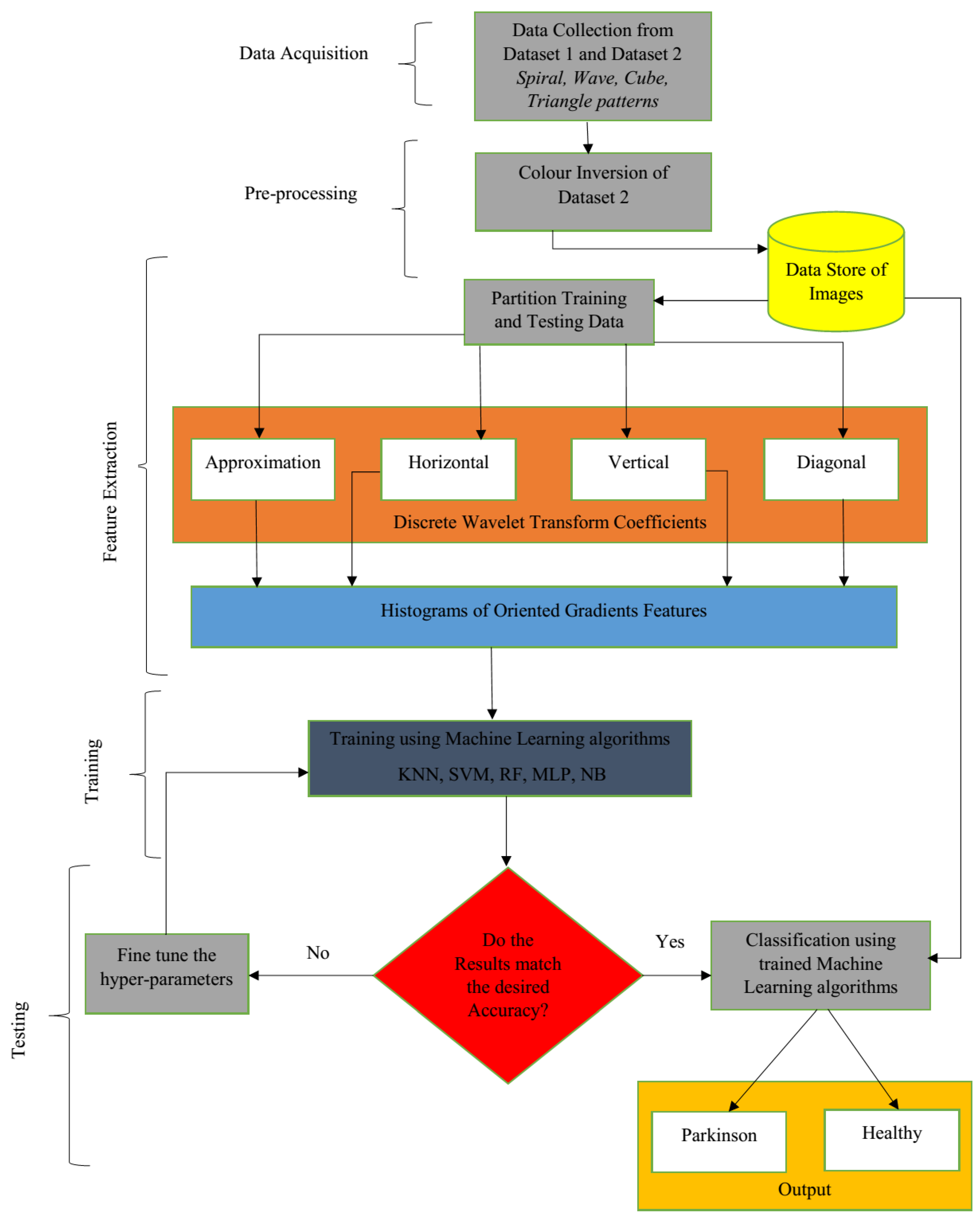
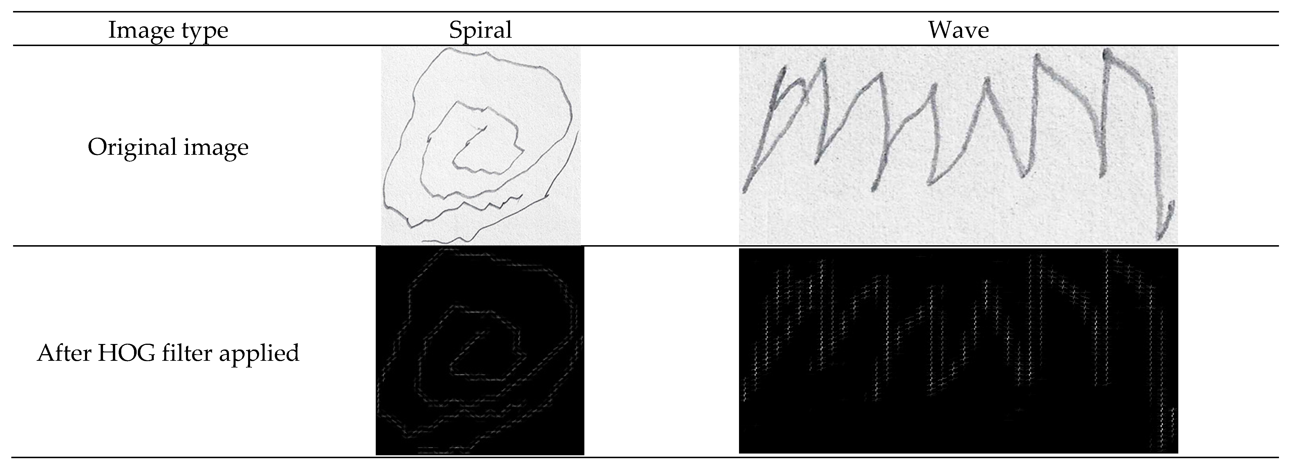
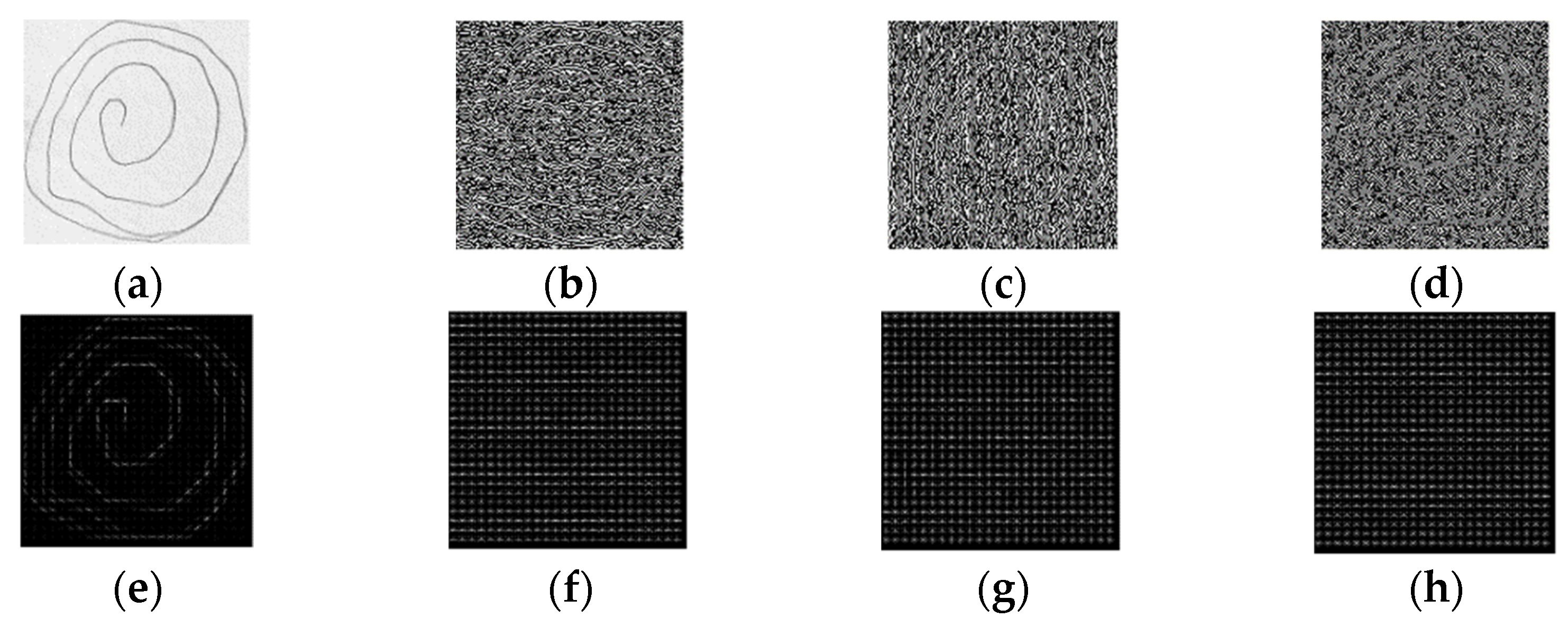
This paper proposes an efficient hybrid fusion-based approach for the early detection of Parkinson’s disease using hand-drawn images. The goal of this work was to use hand-drawn artworks to detect Parkinson’s disease patients, using the fusion of discrete wavelet transform (DWT) coefficients and HOG features, and several classification techniques were utilized to test the efficacy of the proposed model. HOG features are widely used in computer vision tasks for object detection. The HOG descriptor focuses on the structure or the shape of an object. The working dataset consisted of spiral and wave images, where investigation requires not only edge features, but also edge direction, which can be extracted by the HOG descriptor only using the gradients in both the x and y directions. Wavelet transforms are useful for image processing to accurately analyze the abrupt changes in the image that localize means in time and frequency. Wavelets exist for a finite duration, and they have different sizes and shapes. This work also evaluated the performance of various classifiers, using a variety of performance metrics, such as accuracy, precision, specificity, sensitivity, and F-score. The main contribution of this paper lies in the following aspects:
The main focus is on the early detection of Parkinson’s disease with the help of hand-drawn images, which will reduce the high cost of laboratory examinations and will be useful for poor people who cannot bear the extreme cost of clinical examinations.
In continuation from our earlier work, in this work, along with HOG features, DWT coefficients were also explored, and a fusion strategy of feature refinement was exploited.
The proposed models were evaluated on two different datasets composed of various types of patterns.
The targets were to first identify which type of image was more useful, the impact of higher number of images, which dataset gave better results, and which classification technique would be more useful for this work.
This study is structured as follows:
Section 2 explains the database along with the proposed mechanism.
Section 3 explains the experimental results of the proposed model, followed by the discussion in
Section 4. Finally, the conclusion of the paper is presented in
Section 5.
3. Results
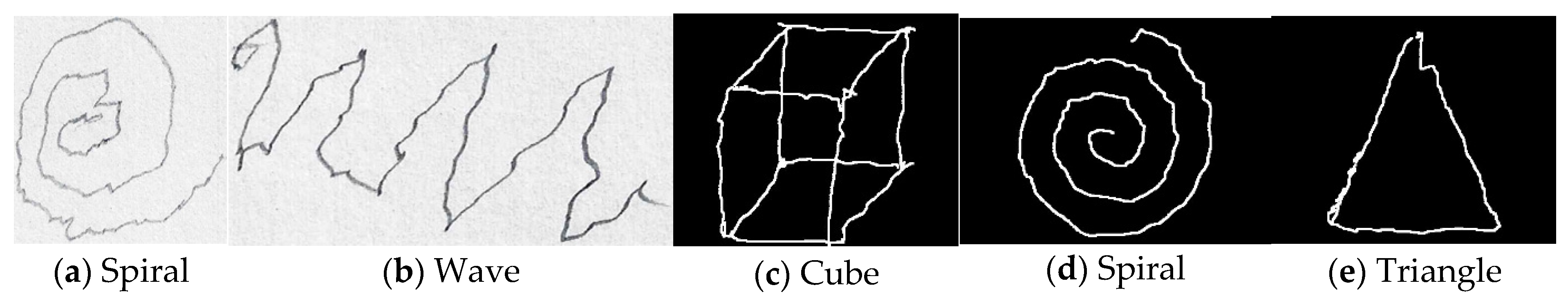
To confirm the efficacy of each picture form, the proposed experimental investigation was conducted in two phases. Comparable images from many categories, such as spiral, wave, triangle, and cube, were trained and assessed in the first phase. The model was then evaluated using a random figure in the second stage, which used a combination of various categories of images from the relevant dataset in the training phase.
For the classification task, we used the following metrics to check the performance of each classifier. From the confusion matrix, we obtained the following parameters: (a) true positives (TP), (b) false negatives (FN), (c) true negatives (TN), and (d) false positives (FP).
Table 2 shows the various performance metrics evaluated to check the efficiency of the proposed model in this work.
3.1. Using Only Approximation Coefficient of DWT with HOG
3.1.1. Dataset 1
Table 3,
Table 4,
Table 5,
Table 6 and
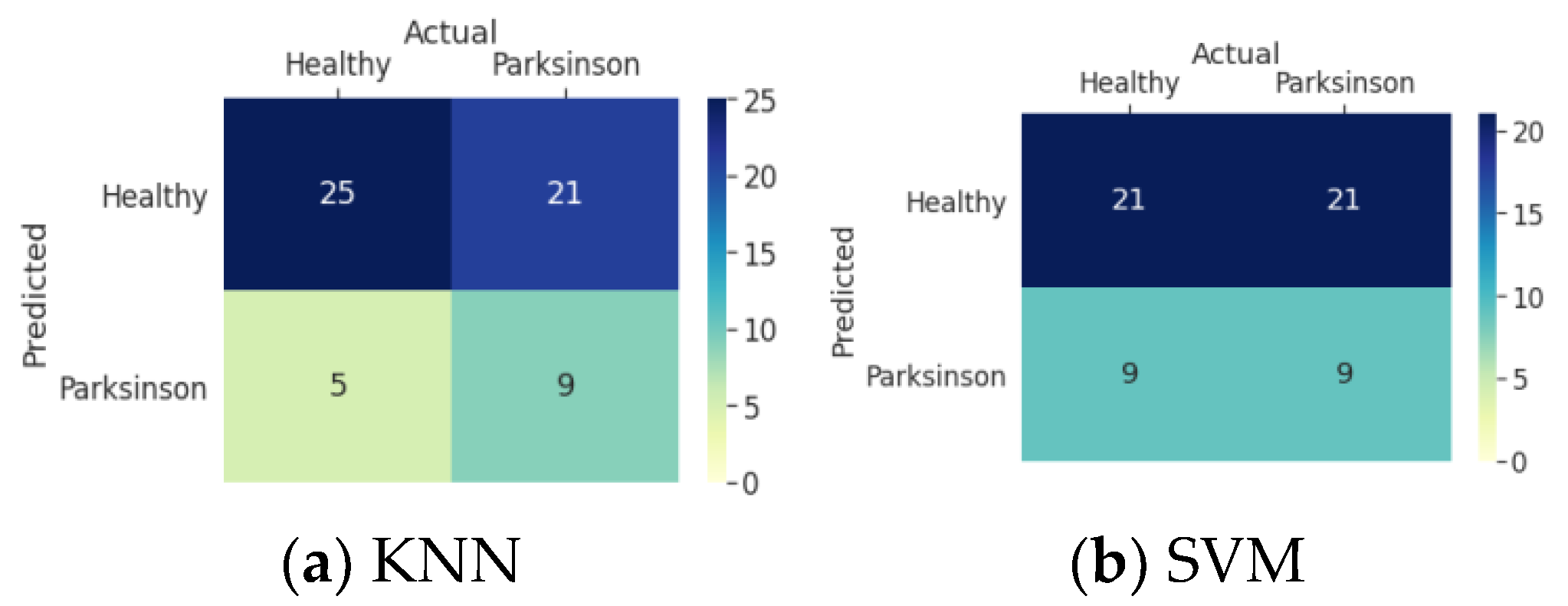
Table 7 contain the result sets for spiral and wave images, as well as a mixture of spiral and wave images, from when HOG features were extracted from only the approximation coefficient. From
Table 3 and
Table 4 of spiral and wave images, the spiral images showed a maximum possible recognition rate of 81.3%, and from
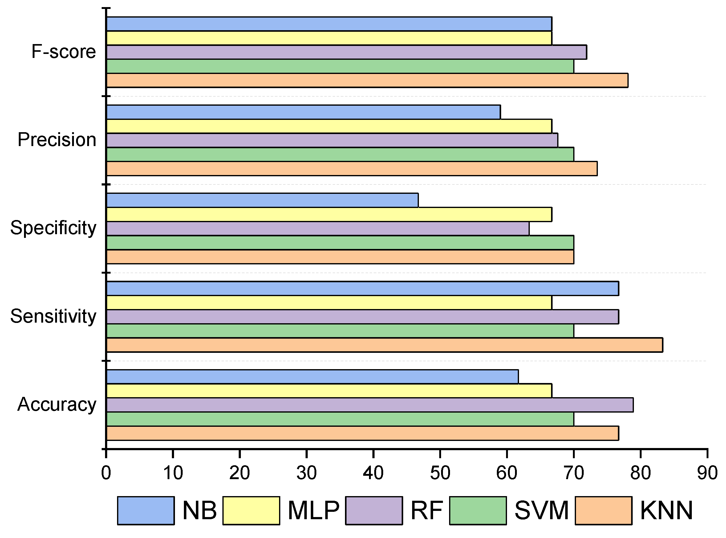
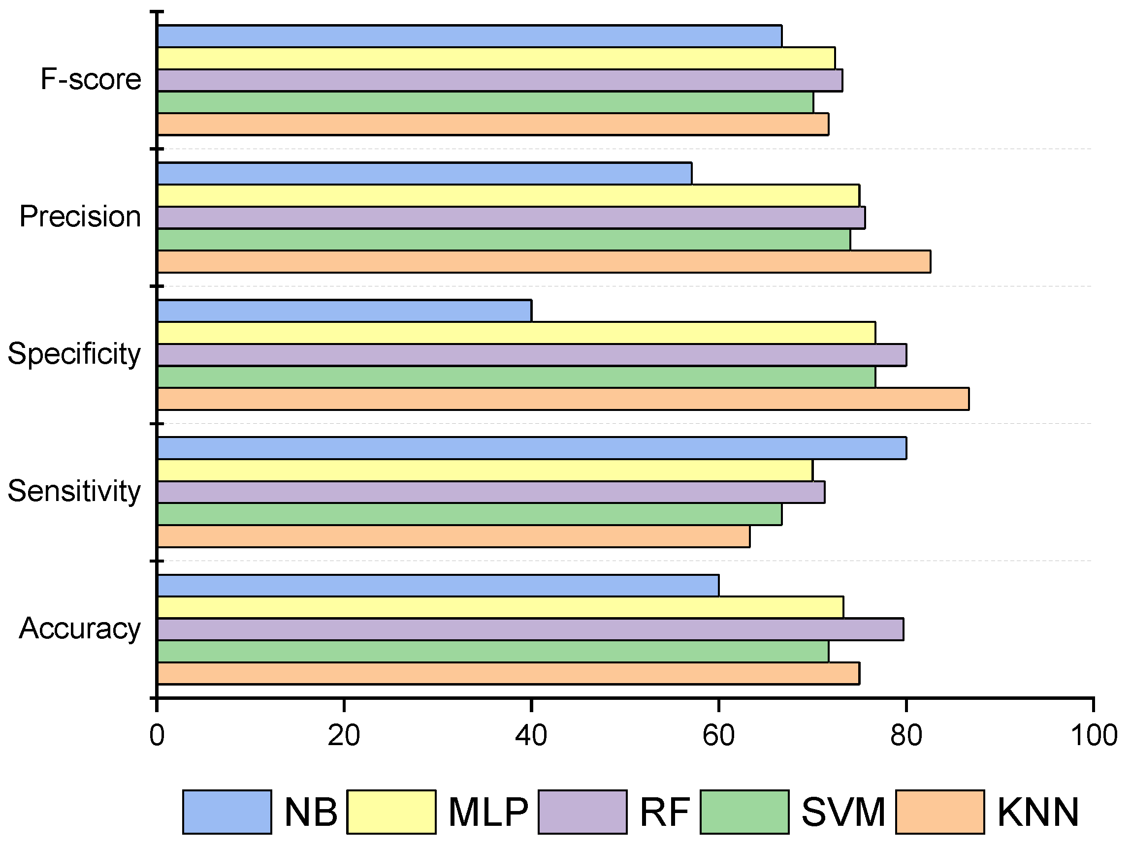
Figure 5 and
Figure 6, it can be seen that the overall RF algorithm gave the most accurate result, with an accuracy of 78.9%.
Table 3.
Results of five machine learning algorithms using spiral images.
Table 3.
Results of five machine learning algorithms using spiral images.
| | KNN (%) | SVM (%) | RF (%) | MLP (%) | NB (%) |
|---|
| Accuracy | 73.3 | 76.7 | 81.3 | 73.3 | 56.7 |
| Sensitivity | 80.0 | 80.0 | 70.7 | 73.3 | 86.7 |
| Specificity | 66.7 | 73.3 | 85.3 | 73.3 | 26.7 |
| Precision | 70.6 | 75.0 | 83.1 | 73.3 | 54.2 |
| F-score | 75.0 | 77.4 | 76.3 | 73.3 | 66.7 |
Table 4.
Results of five machine learning algorithms using wave images.
Table 4.
Results of five machine learning algorithms using wave images.
| | KNN (%) | SVM (%) | RF (%) | MLP (%) | NB (%) |
|---|
| Accuracy | 80.0 | 70.0 | 80.3 | 66.7 | 43.3 |
| Sensitivity | 86.7 | 73.3 | 86.7 | 66.7 | 40.0 |
| Specificity | 73.3 | 66.7 | 62.7 | 66.7 | 46.7 |
| Precision | 76.5 | 68.8 | 68.4 | 66.7 | 42.9 |
| F-score | 81.3 | 71.0 | 76.5 | 66.7 | 41.4 |
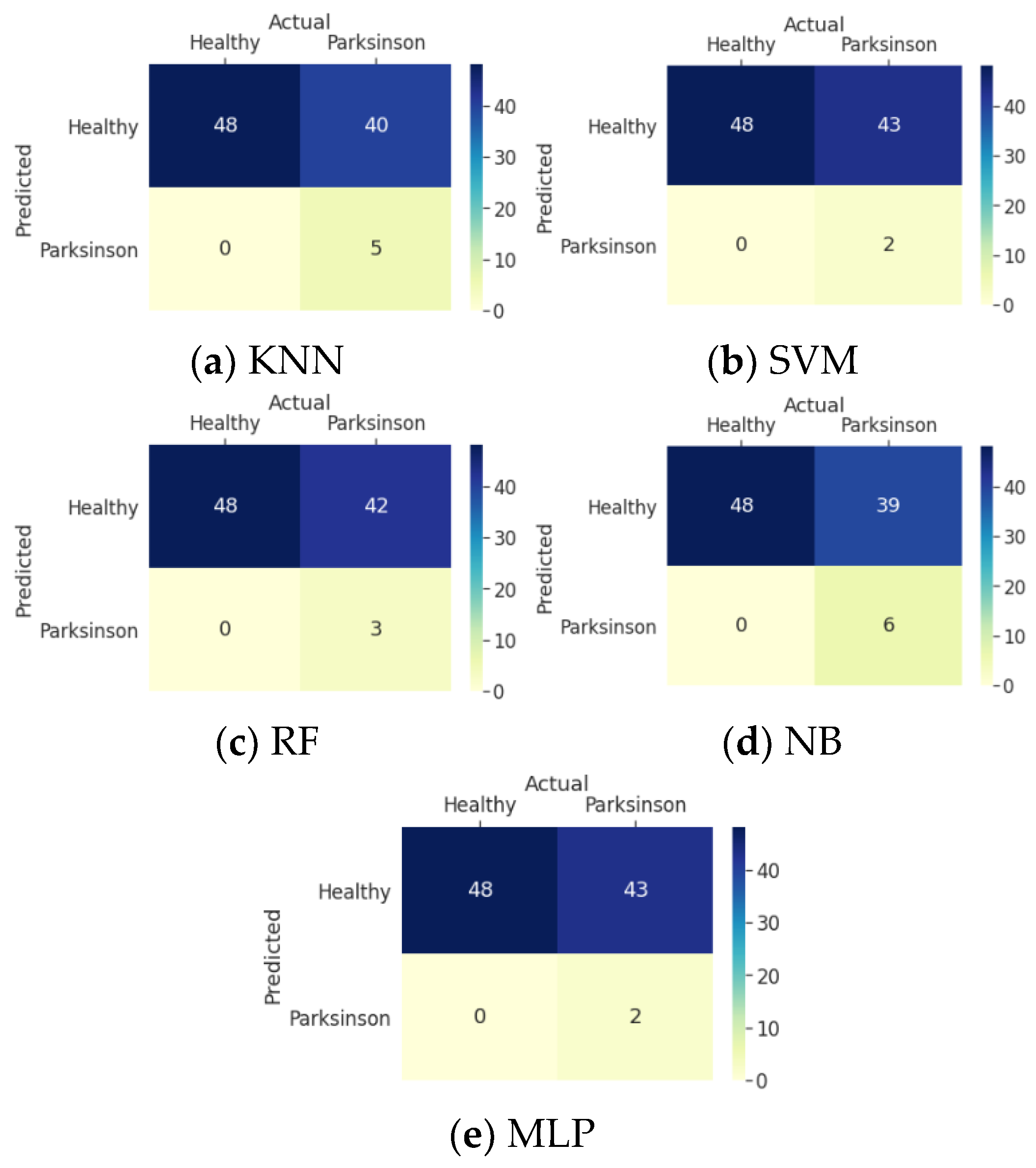
Figure 5.
Confusion matrices (a–e) for approximation coefficient from dataset 1.
Figure 5.
Confusion matrices (a–e) for approximation coefficient from dataset 1.
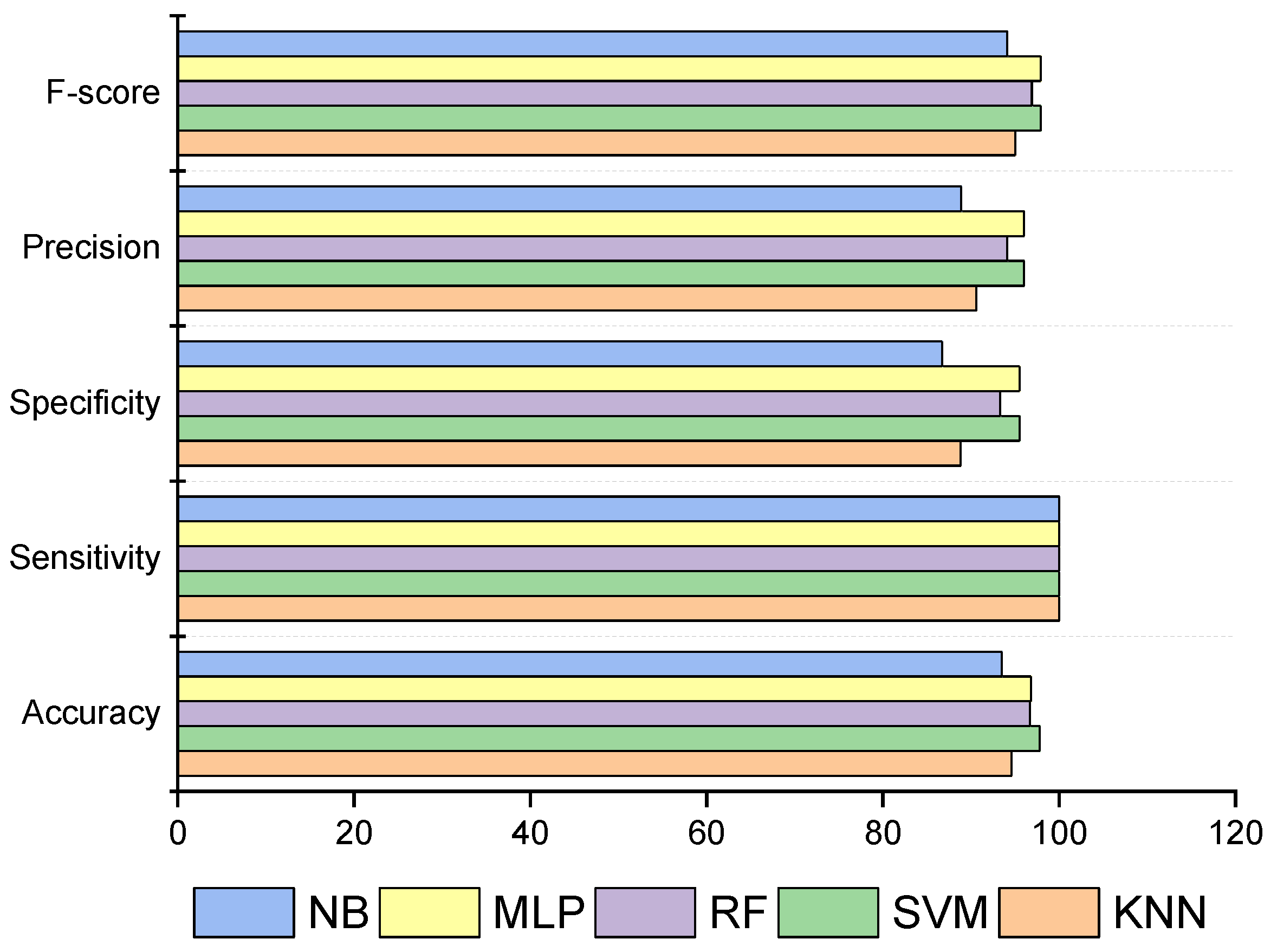
Figure 6.
Performance summary of dataset 1 (%).
Figure 6.
Performance summary of dataset 1 (%).
Table 5.
Results of five machine learning algorithms using spiral images.
Table 5.
Results of five machine learning algorithms using spiral images.
| | KNN (%) | SVM (%) | RF (%) | MLP (%) | NB (%) |
|---|
| Accuracy | 79.2 | 95.8 | 87.5 | 95.8 | 87.5 |
| Sensitivity | 100 | 100 | 100 | 100 | 83.3 |
| Specificity | 16.7 | 83.3 | 50.0 | 83.3 | 100 |
| Precision | 78.2 | 94.7 | 85.7 | 94.7 | 100 |
| F-score | 87.8 | 97.3 | 92.3 | 97.3 | 90.9 |
Table 6.
Results of five machine learning algorithms using cube images.
Table 6.
Results of five machine learning algorithms using cube images.
| | KNN (%) | SVM (%) | RF (%) | MLP (%) | NB (%) |
|---|
| Accuracy | 100 | 100 | 100 | 100 | 100 |
| Sensitivity | 100 | 100 | 100 | 100 | 100 |
| Specificity | 100 | 100 | 100 | 100 | 100 |
| Precision | 100 | 100 | 100 | 100 | 100 |
| F-score | 100 | 100 | 100 | 100 | 100 |
Table 7.
Results of five machine learning algorithms using triangle images.
Table 7.
Results of five machine learning algorithms using triangle images.
| | KNN (%) | SVM (%) | RF (%) | MLP (%) | NB (%) |
|---|
| Accuracy | 94.8 | 94.7 | 91.7 | 91.7 | 91.6 |
| Sensitivity | 100 | 100 | 100 | 100 | 100 |
| Specificity | 83.3 | 66.7 | 73.3 | 66.7 | 66.7 |
| Precision | 94.7 | 90.0 | 91.9 | 90.0 | 90.0 |
| F-score | 97.3 | 94.7 | 95.7 | 94.7 | 94.7 |
3.1.2. Dataset 2
From
Table 5,
Table 6 and
Table 7, it is clearly visible that, for the approximation coefficient, cube images are the most suitable ones, and from
Figure 7 and
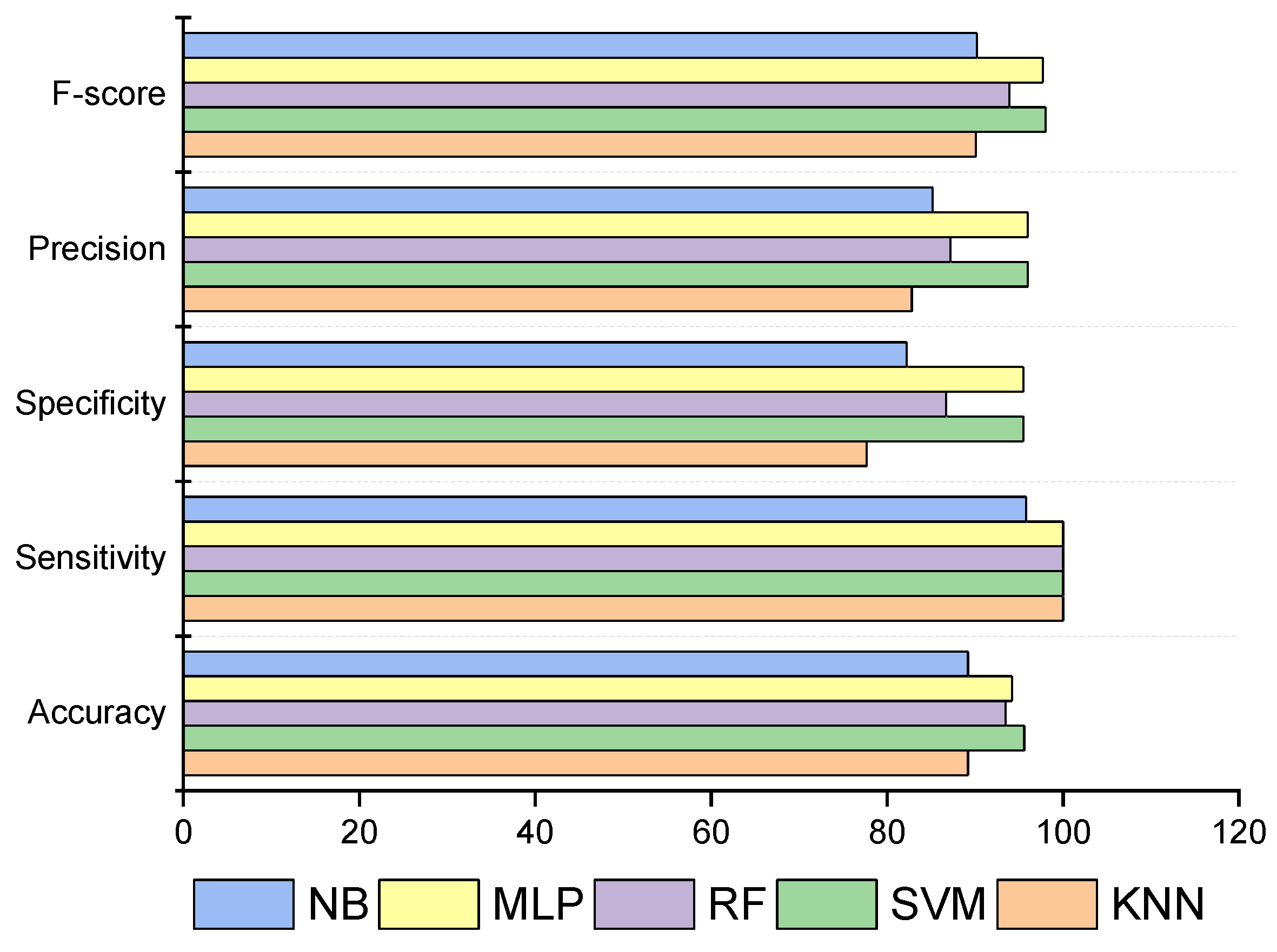
Figure 8, it can be concluded that overall SVM performed best for dataset 2, with an accuracy of 95.6%.
3.2. Using All Four DWT Coefficients with HOG
Table 8,
Table 9,
Table 10,
Table 11 and
Table 12 contain the result sets for spiral, cube, and triangle images, as well as a mixture of spiral, cube, and triangle images, from when HOG features were extracted from all four DWT coefficients, which are approximation, horizontal, vertical, and diagonal.
3.2.1. Dataset 1
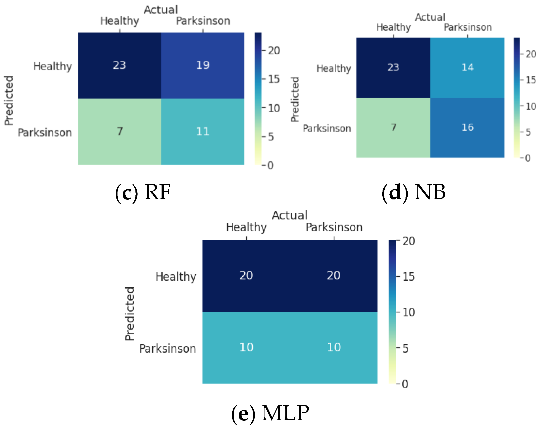
From
Table 8 and
Table 9 of spiral and wave images, the spiral images showed a maximum possible recognition rate of 82.7%, and from
Figure 9 and
Figure 10, we can conclude that overall RF achieved 79.7% accuracy.
Table 8.
Results of five machine learning algorithms using spiral images.
Table 8.
Results of five machine learning algorithms using spiral images.
| | KNN (%) | SVM (%) | RF (%) | MLP (%) | NB (%) |
|---|
| Accuracy | 70.0 | 76.7 | 82.7 | 76.7 | 53.3 |
| Sensitivity | 53.3 | 80.0 | 73.3 | 80.0 | 93.3 |
| Specificity | 86.7 | 73.3 | 86.7 | 73.3 | 13.3 |
| Precision | 80.0 | 75.0 | 84.6 | 75.0 | 51.8 |
| F-score | 64.0 | 77.4 | 78.6 | 77.4 | 66.7 |
Table 9.
Results of five machine learning algorithms using wave images.
Table 9.
Results of five machine learning algorithms using wave images.
| | KNN (%) | SVM (%) | RF (%) | MLP (%) | NB (%) |
|---|
| Accuracy | 73.3 | 73.3 | 76.7 | 73.3 | 53.3 |
| Sensitivity | 60.0 | 66.7 | 80.0 | 66.7 | 53.3 |
| Specificity | 86.7 | 80.0 | 73.3 | 80.0 | 53.3 |
| Precision | 81.8 | 76.9 | 75.0 | 76.9 | 53.3 |
| F-score | 69.2 | 71.4 | 77.4 | 71.4 | 53.3 |
Figure 9.
Confusion matrices (a–e) for all DWT coefficients from dataset 1.
Figure 9.
Confusion matrices (a–e) for all DWT coefficients from dataset 1.
Figure 10.
Performance summary of dataset 1 (%).
Figure 10.
Performance summary of dataset 1 (%).
3.2.2. Dataset 2
From
Table 10,
Table 11 and
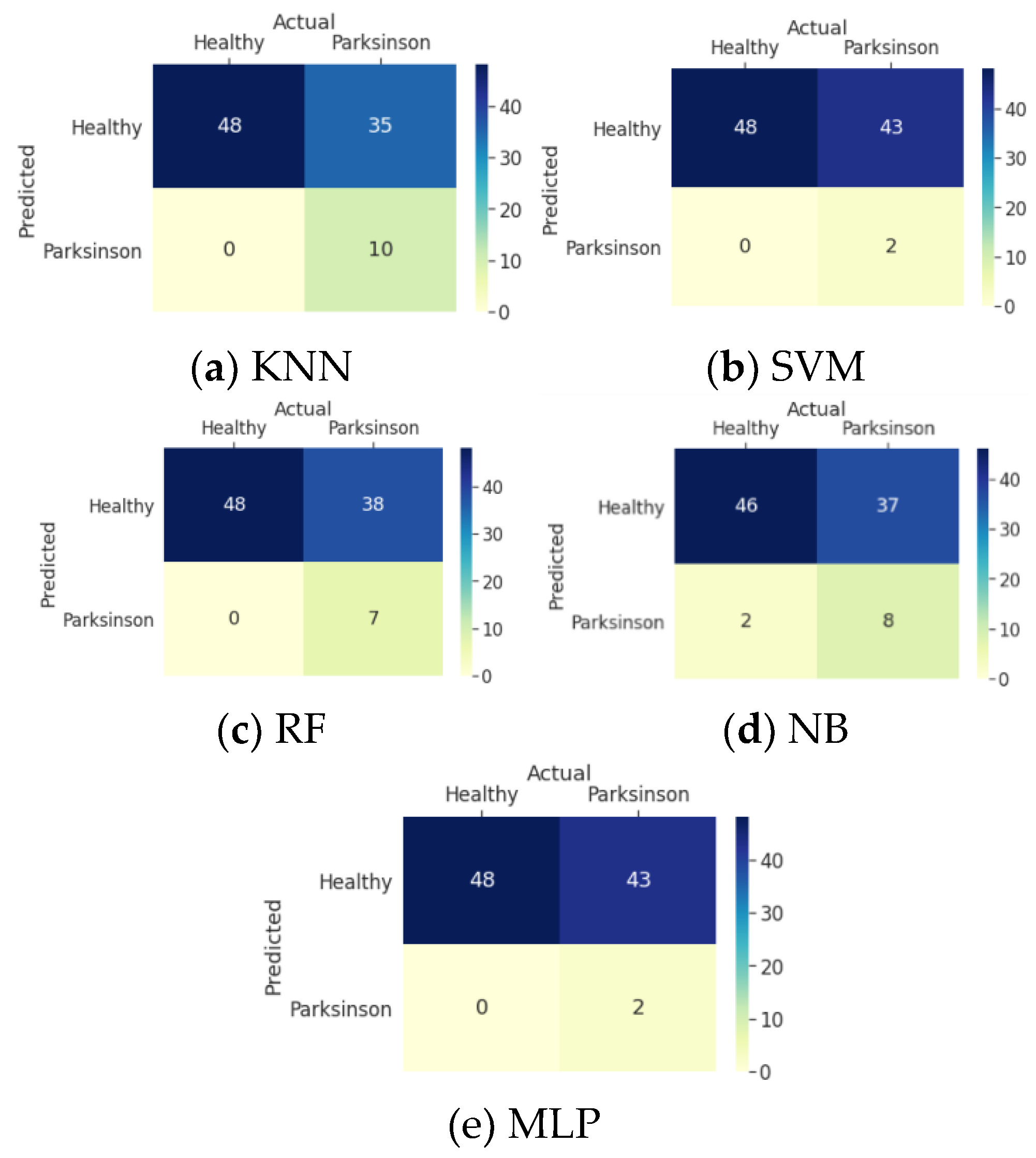
Table 12, we can conclude that for all four coefficients, the cube images achieved maximum accuracy, and from
Figure 11 and
Figure 12, it can be seen that overall SVM achieved an accuracy of 97.8%.
Table 10.
Results of five machine learning algorithms using spiral images.
Table 10.
Results of five machine learning algorithms using spiral images.
| | KNN (%) | SVM (%) | RF (%) | MLP (%) | NB (%) |
|---|
| Accuracy | 87.5 | 95.8 | 95.8 | 95.8 | 95.8 |
| Sensitivity | 100 | 100 | 100 | 100 | 100 |
| Specificity | 50.0 | 83.3 | 83.3 | 83.3 | 83.3 |
| Precision | 85.7 | 94.7 | 94.7 | 94.7 | 94.7 |
| F-score | 92.3 | 97.2 | 97.2 | 97.2 | 97.2 |
Table 11.
Results of five machine learning algorithms using cube images.
Table 11.
Results of five machine learning algorithms using cube images.
| | KNN (%) | SVM (%) | RF (%) | MLP (%) | NB (%) |
|---|
| Accuracy | 100 | 100 | 100 | 100 | 100 |
| Sensitivity | 100 | 100 | 100 | 100 | 100 |
| Specificity | 100 | 100 | 100 | 100 | 100 |
| Precision | 100 | 100 | 100 | 100 | 100 |
| F-score | 100 | 100 | 100 | 100 | 100 |
Table 12.
Results of five machine learning algorithms using triangle images.
Table 12.
Results of five machine learning algorithms using triangle images.
| | KNN (%) | SVM (%) | RF (%) | MLP (%) | NB (%) |
|---|
| Accuracy | 95.8 | 91.7 | 91.7 | 91.7 | 91.7 |
| Sensitivity | 100 | 100 | 100 | 100 | 100 |
| Specificity | 83.3 | 66.7 | 66.7 | 66.7 | 66.7 |
| Precision | 94.7 | 90.0 | 90.0 | 90.0 | 90.0 |
| F-score | 97.2 | 94.7 | 94.7 | 94.7 | 94.7 |
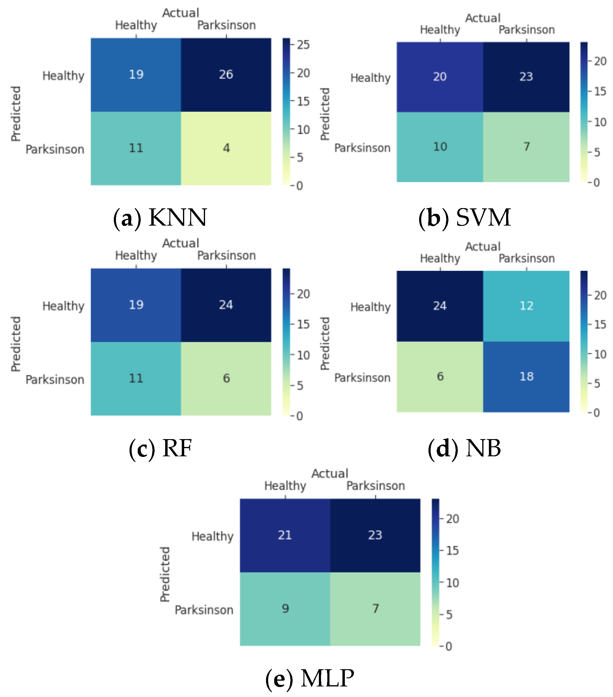
Figure 11.
Confusion matrices (a–e) for all DWT coefficients from dataset 2.
Figure 11.
Confusion matrices (a–e) for all DWT coefficients from dataset 2.
Figure 12.
Performance summary of dataset 2 (%).
Figure 12.
Performance summary of dataset 2 (%).
4. Discussion
From the experimental results, it can be concluded that the fusion-based features surpassed the result obtained using only the approximation coefficient. Folador et al. [
8] utilized the HOG descriptor in conjunction with a random forest classifier to accurately distinguish between persons with Parkinson’s disease and those who are healthy. They achieved a highest accuracy, sensitivity, and specificity classification success rates of 83%, 85%, and 81%, respectively. In our previous work [
9], we evaluated the performance of different machine learning algorithms using only the features extracted from HOG descriptors for hand-drawn images. It was found that for dataset 1 and dataset 2, the proposed model was able to achieve a highest accuracy of 74.7% and 96.8%, respectively.
To further enhance the previous results, in this work, two different approaches were compared. The key feature of this work is that DWT coefficients were extracted first, and on top of that, HOG features were extracted for feature refinement; thereafter, the extracted features were fed to the different machine learning algorithms. In DWT coefficients, there are also various types of coefficients; therefore, in this work, the efficiency of those coefficients was also evaluated. One experimental approach was to extract using the approximation coefficient, and the other one was with all the four coefficients. An analysis was performed for the approximation coefficient against all coefficients. From the findings, it can be concluded that the second approach outperformed the first approach.
Table 13 shows the accuracy performance comparison of the proposed approaches with other state-of-the-art techniques.
5. Conclusions
In this work, we adopted a fusion technique, combining discrete wavelet transform coefficients and histograms of oriented gradient features to detect Parkinson’s disease from the hand-drawn images drawn by Parkinson’s disease-affected patients. It outperformed the same experiment that was performed with only histograms of oriented gradient features. The main purpose of this research was to extract relevant information from discrete wavelet transform coefficients and identify the most important coefficients. In addition, a fusion technique was used to compare the performance of the approach to previous work that exclusively used histograms of oriented gradient characteristics. The results of the experiments show that fusion-based features outperform the outcome produced using merely the approximation coefficient. In our earlier work, we examined the effectiveness of several machine learning techniques for hand-drawn pictures, using just the features retrieved from histograms of oriented gradient descriptors. For datasets 1 and 2, an accuracy of 74.7% and 96.8%, respectively, was attained solely using histograms of oriented gradient features on various machine learning methods. In order to improve on the prior findings, two distinct methodologies were examined in this research. The main characteristic of this work is that discrete wavelet transform coefficients were extracted first, followed by histograms of oriented gradient features for feature refinement, and finally, the extracted features were fed as input to various machine learning methods. There are numerous sorts of coefficients in the discrete wavelet transform; thus, the effectiveness of various coefficients was also investigated in this work. The first method was to extract using only the approximation coefficient, and the second method was to extract using all four coefficients. The approximation coefficient was compared against other discrete wavelet transform coefficients, such as horizontal, vertical, and diagonal. According to the findings of the experiments, the second strategy obtained 76.7% and 97.4% accuracy for dataset 1 and dataset 2, respectively. Another conclusion is that random forest and support vector machine classifiers had the most promising outcomes when compared to other classifiers; out of different kinds of hand-drawn figures, spiral pattern images showed the best performance. The suggested method has a restriction because there is not as much data for the hand-drawn images. With a larger amount of data, the robustness of the proposed models could have been tested. While the experimental results for the small dataset scenario are encouraging, more work can be performed to expand the datasets using augmentation techniques. With more image classes being available, we may develop deep learning models for the better detection of features.


 ,
, 


