Abstract
An algorithm is derived for active business management. The key component of the algorithm is the definition and solution of an appropriate portfolio problem. For the last one, the disbursements for the business management are regarded as potential portfolio resources. For the portfolio definition, the increases or decreases of the disbursements are assumed to be the assets, whose weights are found as solutions from the portfolio optimization problem. These solutions recommend the reallocation of the resources between different disbursements, which increases the income of the business entity. The definition and solution of this portfolio problem are made sequentially in time, and the obtained solutions are applied as recommendations for future business management steps. An algorithm for business management, based on the sliding mode of repetitive definitions and solutions of portfolio problems with historical data of last disbursements, gives recommendations for the reallocation of resources for the next future period of management. The algorithm is numerically tested with real data on animal husbandry from Bulgaria. The empirical results demonstrate an advantage in increasing the husbandry income in comparison with the lack of such an active business policy. The algorithm can be implemented as a software solution in an appropriate programming system, supporting fintech service for active business management.
MSC:
91B28; 91B32; 68W01
1. Introduction
The main approach in this paper is to motivate that the business management decisions have to be based on quantitative assessments and solutions. Quantitative solutions can be found by applying an optimization approach by definition and solution of an appropriate optimization problem. This research targets the usage of quantitative models, which are applied to the business management of animal husbandry. It is chosen quantitative modeling and optimization to be performed in the framework of the portfolio theory. Thus, business management will be performed under two important criteria for maximization of return and minimization of risk. Our research targets an approach coming from the fintech domain for the usage and application of information technology solutions in business management activities. Thus, our application of the portfolio theory will result in deriving an algorithm for business management. The existence of a working algorithm gives the opportunity for parts of the business management decisions to be performed in an automatic way by the usage of software tools, which implement the algorithm derived in this paper.
This research is based on the overlapping points between the topics of business management, the fintech domain, and portfolio modeling. The overview below tries to point out cases that can illustrate the power of business solutions, which can benefit from the application of a quantitative business approach, applied in an algorithmic sequence for optimal management of a business and production entity.
To clear the content of business management, we use the definition of management science as “the broad interdisciplinary study of problem-solving and decision making in human organization, with strong links to management, economics, business, engineering, management consulting and other fields” [1]. Business management is an important domain of management science, and its roots come in the early years of the last century [2]. This kind of management applies methods that are related to analyzing and modeling business processes [3]. Business management, in general, contains different elements, which are described mainly in a qualitative way. For example, in [4], six general elements of business management are outlined: strategic alignment, governance, methods, information technology, people, and culture. These elements are qualitatively assessed and estimated by the components, which have to be performed for their satisfaction. In [5], one can find descriptions of six main functional areas for applications of business management: people management; operation management of production process; accounting for management of finances; strategy management as high-level business entity control; data analytics, targeting the optimization of the business performance; marketing, which includes advertising and social media presence. It exists wider forms of decomposition of the business functional management. For illustration, Ref. [6] defines purchase function; productivity; personnel function; research and development; financial management, and economics.
This paper does not claim an extended overview of the application domains of business management nor the content of its functions. This short reference tries to illustrate that the main contents of the business management activities are mainly described in a qualitative descriptive way.
The benefit of business management generally comes from quantitative decisions and recommendations. In our work, we generally pay attention to quantitative solutions, which can be derived and implemented in real business cases. Our approach to quantification of business decisions is directed towards the financial management of a business entity that has production activities of goods.
The contributions of this paper concern the quantitative approach, which is applied to considering decision making for business management. This is achieved by the definition and solution of a portfolio optimization problem. As portfolio assets, a set of disbursements of the production activities of a business entity are regarded. The portfolio problem addresses the increase or decrease in the disbursements by means of increasing the income without having additional resources for disbursements. The portfolio solutions recommend the reallocation of the available resource. This portfolio problem is incorporated in an algorithm, which targets the increase in income by reallocation of resources. The empirical results confirm the benefit of the derived algorithm. The rest of the paper is organized as follows: in Section 2, an analysis of the quantitative models for business management is given. In Section 3, key elements of the portfolio theory are discussed. In Section 4, our model for the portfolio problem, addressing the increase or decrease in income, is derived. In Section 5, the algorithm is presented, which incorporates the usage of the portfolio problem. In Section 6, the rules for the application of the algorithm are presented. Section 7 gives numerical results of the empirical experiments with real data. Section 8 discusses the obtained results and the potential for improving and complicating the algorithm. Finally, Section 9 concludes this paper.
2. Quantitative Models for Business Management and Applications of Portfolio Theory
The quantitative models in business management provide analysis of data and support decision making. The quantitative approach allows being found the best solutions, providing efficient decisions. The quantitative solutions are obtained mainly from the application of different parts of mathematics. As an example, in [7], the solutions to a set of problems for business management are illustrated with the application of a linear set of equations, matrix algebra, mathematics of finance, linear programming, network analysis and scheduling, transportation problems, and inventory planning. Quantitative methods for management and decision making in the business domain are discussed in [8]. Our research addresses problems related to the financial management of enterprise resources. This makes it important to discuss the topic of fintech applications for financial services. Fintech refers mainly to the application of information technologies in financial services [9]. An overview of the fintech approaches one can find in [10,11,12]. Following [13], the term fintech appeared at first in business journals. It addresses problems and services in the financial sector. Fintech is defined as a service that applies information technology, supporting the financial domain [14,15]. An important part of fintech solutions is the development and implementation of algorithmic and software components for fintech services. Thus, information technologies are the backbone for the implementation of new financial services and decision solutions in this domain. For example, Fintech services are related to the domains of credit reports, digital banking, insurance, investing, lending, payments, real estate, and risk analysis [13]. Because our primary goal of this research is to provide info service to a production business management, our approach is to model the production process as a sequence of investment decisions. We assume that all disbursements made for a production process have to be assumed as an appropriate form of investment. The investment decisions are quantified under the approaches of the portfolio optimization theory [16]. Thus, our research deals with the development of models and algorithms, which basically use formal descriptions from the portfolio theory.
The portfolio theory has been launched with the famous works of [16]. We mention important stages of its development with the works of [17,18]. In [16], the formal optimization portfolio problem was introduced, which minimizes the risk of the investment, and supports an appropriate level of portfolio return. In [17], the portfolio theory introduced a new portfolio parameter as the market portfolio. Respectively, additional relations for the portfolio have been derived in the so-called Capital Asset Pricing Model. It has introduced new important relations, named Capital Market Line, Security Market Line, and characteristic line. A new step in the development of portfolio theory was the works of Black–Litterman, where additional new parameters were introduced, named “implied returns” [18,19,20]. These new parameters integrate the assessment both from the historical dynamics and the expert expectation for the future levels of the asset returns giving an assessment about the next future levels of the assets. The usage of the “implied returns” according to the Black–Litterman model gives better results in comparison with the classical portfolio model of Markowitz. The portfolio problem has been extended with additional constraints by means to reflect real business cases with transactional costs. Respectively the cardinality constraints, with nixed integer constraint, reduce the size of the assets included in the portfolio.
An extension of the term risk and its formal presentation was the definition of the parameter Value at Risk (VaR) [21]. Respectively, the portfolio model can accommodate risk with two formal descriptions with the value of variance and VaR of the portfolio return and/or loss and its derivative form Conditional VaR (CVaR). The portfolio problem is complicated in [22] by the application of CVaR in a goal function of the portfolio problem, defined as an appropriate Sharpe ratio. The portfolio problem takes additional cardinality constraints. The resulting portfolio problem is solved with neuro dynamic optimization due to its complexity.
The analysis above targets to convince the reader that the portfolio theory has its own way of development, which increases its potential for quantitative decisions and management recommendations. The portfolio theory is successfully applied for the assessment of the economic value of business management because it gives a universal metric for the comparison of different business applications [23].
Nevertheless, that portfolio theory is applied in financial and investment domains, and its quantitative models are used in different cases and applications. In [24], portfolio formalism is used in solving the problem of structural choice, which gives a structural diagnosis for resource distribution. In [25], the Capital Asset Pricing Model is quantitatively applied for fintech decisions, increasing the number of factors taken into consideration in the investment process. The portfolio mean-variance modeling is applied for the integration of healthcare services [26]. In [27], the portfolio theory is used to disperse the supply chain, finding efficient supplier combinations.
A trading algorithm based on portfolio theory is discussed in [28]. The portfolio theory is applied to choosing a combination of wheat, which enhances the profitability over the selection of a single sort of wheat [29]. Commercial real estate portfolios are analyzed with quantitative categories of the portfolio theory in [30]. A solution for decreasing the risk in the agriculture domain is performed by the application of the portfolio theory [31]. The application of quantitative modeling of business management is assessed and evaluated in [32,33]. The stock process of companies for the development of e-business services is predicted and managed, applying portfolio modeling and optimization to assess the future behavior of the e-business [34]. Purchasing decisions for procurement and supply chains by applying portfolio modeling are given in [35]. Improvements in pension plans by foreign assets are also evaluated on portfolio formalism [36].
This sequence of applications of the portfolio theory proves and gives evidence that portfolio formalism is a powerful tool for the quantification of decision making in managing different forms of business activities. Next, we introduce the key points of the portfolio theory, which we use in the next sections of the paper.
3. Formal Background of the Portfolio Theory
The basic input parameters for the portfolio problems are the records of the historical returns of the assets, which will participate in the portfolio
where N is the number of assets, and n is the length of the historical period. is the current return of asset i for the time (j).
The initial set of data R allows evaluating three important statistical characteristics of the assets returns:
- -
- Mean value of the return:
- -
- Standard deviations:
- -
- Covariance square matrix Σ, N × N between the asset returns Ri, Rj, i, j, 1 = N:
The portfolio theory assumes that the standard deviations, together with the covariance, are quantitative measures for the risk of each asset as of the portfolio, which is a combination of the assets.
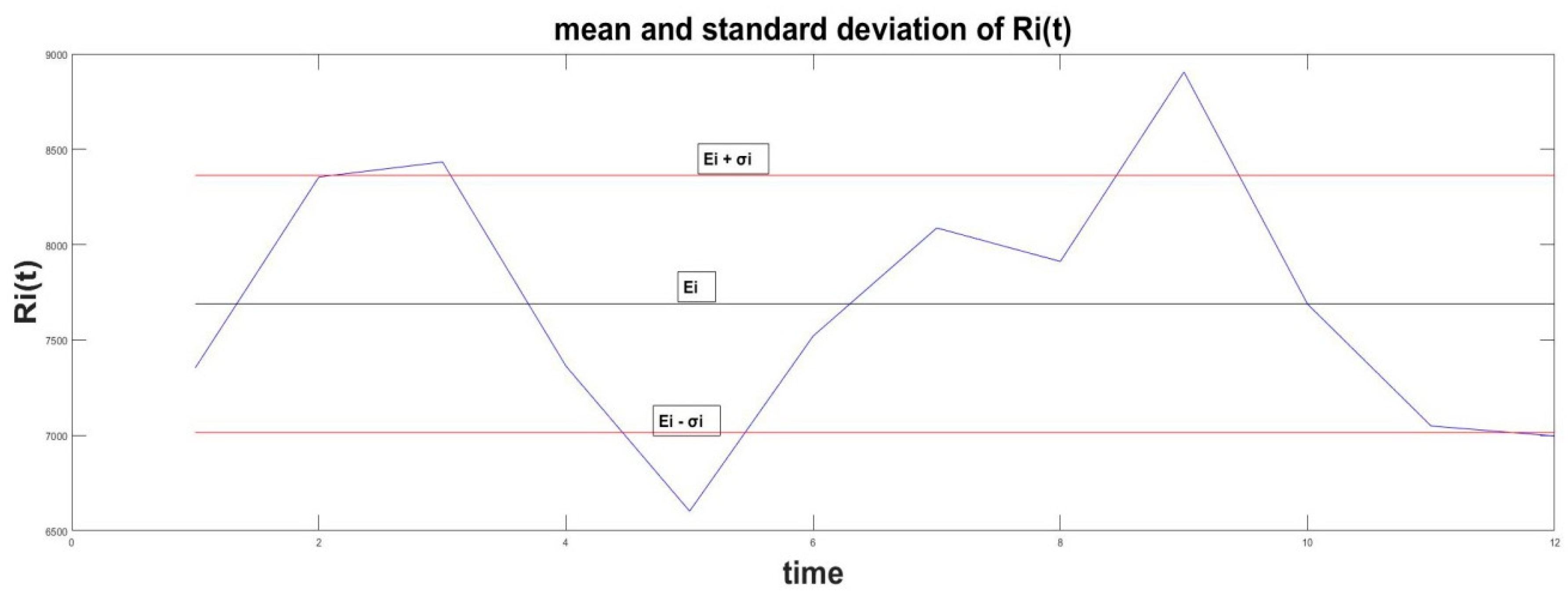
The risk interpretation comes from the statistics [37], given that the predominant set of the real returns Ri(t) will belong to the set of values given by the inequality
This relation says that the probability that the values of returns Ri(t) belong to the space [Ei − , Ei + ] is about 68%. Not all values of Ri(t) will be there, but the predominant amount of them will belong to this diapason. The graphical interpretation of this relation is given in Figure 1.
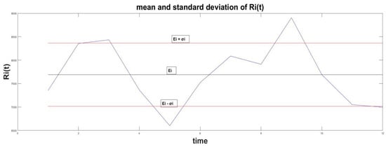
Figure 1.
Illustration between the mean , standard deviation , and stochastic value Ri(t).
Hence, if the standard deviation has a small value, then the real value of the return Ri(t) will be close to the mean estimation and the decision maker can use this value as a forecast for the future level of asset return.
These asset parameters are used for the evaluation of the portfolio return and risk. Because the portfolio is a combination of assets, its return and risk depend on the weights wi, i = 1, N of each asset, how many amounts of it participates in the portfolio
where is the portfolio return, —portfolio risk, Σ—covariance matrix of the asset returns.
For the weights wi a normalization equation is applied
With such defined portfolio relation, the optimization problem, which evaluated the optimal weights of assets in the portfolio, can be evaluated by the portfolio problem
The next step of the portfolio theory comes from the definition and inclusion of a new term, named market return EM and market risk [17]. This new parameter has been formally related to the risks and returns of the portfolio and assets. Thus, coming from the Capital Asset Pricing Model, the following formal relations are introduced in the portfolio theory:
where is the return of the risky free asset.
The CML gives an assessment of the possible relation between the portfolio return and risk for the particular market, which has market return EM and market risk . Particularly the assessment of these values (EM, ) comes from the values of the index of the corresponding market.
where .
The SML gives straight relation between the market return EM and the return of the individual asset Ei. The coefficient depends on the covariance between the return of asset i and this one of the market.
It gives the relation between the current values of the asset return Ri and this one of the market RM. This relation can be used to forecast the level of the asset return Ri according to the value of the current market return RM.
In this research, we use these formal relations from the portfolio theory. Particularly the characteristic line plays an important role in the derived algorithm. This relation plays an important role in the analytical definition of the relations between the portfolio return and the disbursements in the business entity.
To have a more complex view of the analytical relations of portfolio theory, one can refer to the overview [38].
4. Portfolio Model for the Business Management
The particular case, which is under consideration, is the management of animal husbandry. It produces milk and meat from cows, but these products are related to a set of disbursements. The application of the portfolio theory targets the quantification of how much a type of disbursement is to be reduced or increased by means to increase the income of the husbandry. The initial data of incomes and disbursements come from the balance sheets of the husbandry for 3 previous years, 2019, 2020, and 2021.
The disbursements are classified in N = 12 categories: R1 ≡ drugs; R2 ≡ electricity, R3 ≡ salaries, R4 ≡ insurances, R5 ≡ credits, R6 ≡ interest loans, R7 ≡ leasing contracts, R8 ≡ fuel, R9 ≡ repairs, R10 ≡ fodders, R11 ≡ others, and R12 ≡ animal insemination products. The animal husbandry incomes are also estimated per month. Formally the input data of the husbandry production and business are illustrated in Table 1.

Table 1.
Available input data of the husbandry production.
Having these historical data, the management problem concerns the evaluation of the relative increases or decreases of the disbursements Ri = , Ri, i = 1, N, by means to increase the husbandry income RM. The evaluation of the relative weights for increase or decrease is performed by a formal model based on portfolio relations.
From the initial data from Table 1, it is possible to evaluate the mean values of disbursements and the income as their standard deviations as a measure of risk or
To simplify the notations, these values are calculated only for a period of one year, or n = 12 months. Following the portfolio formalism, the characteristic line HC formally is defined as a linear relationship between the current market return RM and the current asset return Ri
where and are coefficients.
The assumptions made in this research take to be the husbandry income and is the corresponding ith disbursement. Because we want to find how disbursement influences the husbandry return, we interchange the roles of and in a formal relation
where and are unknown coefficients. For the evaluation of , one can use two possible solutions.
4.1. Evaluation by the Usage of the Covariance Matrix
Assuming that relation (7) holds for the current values of and this relation has to be valid also for the mean values of EM and Ei of the income and disbursement i or
The covariance between M and i is equal to
Substituting (7) and (8) in (9) gives
Respectively from (8)
The values define the tendencies between the disbursement i in the income M.
If , this means that the increase in the disbursement i will increase the income M.
If , this means that the decrease in the disbursement i will decrease the income M.
4.2. Evaluation by Application of the Least Square Method
The analytical approximation between and is a linear one. The least square method evaluates the unknown coefficients and by a linear system of equations [39]
Thus, using directly the initial data from Table 1, the least square method gives the values of the unknown coefficients and .
Relation (7) gives a formal description of the influence of each disbursement towards the income . Because we need to find the simultaneous influences of all to the income we derive such analytical relation in the following way, taking into consideration that (7) is also valid for the mean values and :
4.3. Definition of a Portfolio Problem
Let us start from the derived analytical relation for particular disbursement i, given by the linear relation (8). We assume that due to the manager’s decisions, the disbursement i will change its mean with a relative weight of . Hence, the new value of the income will be equal to
The increase in the income is related to the sign of the coefficient :
- If > 0, the increase in the income is ;
- If < 0, the increase in the income is due to the decrease in disbursement i from relative 1 to (1 − , or .
The increases due to all disbursements i = 1, N can be used in a portfolio problem for the evaluation of the weights for finding how much to increase or decrease the mean value of a corresponding disbursement.
Hence, the portfolio problem targets the maximization of the increase in the income given by all disbursements i = 1, N or formally
Because is a relative increase in disbursement i, such increase has to satisfy the relative relation
because only a few changes of could be eligible.
The portfolio problem takes an analytical form
The portfolio problem (12) can accommodate additional constraints for resource allocation. Such a constraint can insist on the volume of resources, which decreases from disbursement j for which is to be allocated for disbursement i where . Thus additional resources for business management are not used, but by a reorganization of the available ones, the income is increased according to the portfolio problem (12). Formally such additional constraint can take the form
However, this form of the portfolio problem does not consider the risk of the income increase .
4.4. Evaluation of the Risk of the Income Increase
The portfolio theory states that the real increase will belong predominantly in the space
For the portfolio problem, it is needed to find an analytical description of the standard deviation of the income increase , which is a measure of the risk for the income increase . By definition, the volatility of the increase is evaluated as
However,
Respectively,
After substitution (15) and (16) in (14), the last takes the form
To simplify the notations, a matrix form of relations is used
where b = (bq, … bN).
The covariance matrix ∑ is evaluated from the initial data from Table 1 according to relations (4). Using relation (17), the portfolio problem, which minimizes the risk of the increase and maximizes the mean increase takes the analytical form
This portfolio problem incorporates both the risk and return in a single analytic relation, known as the Sharpe ratio [17]. Towards this portfolio, problem relation (13) can be added as a constraint, which means that there are no additional investment resources for the portfolio. Portfolio problem (18) is incorporated in an algorithm, which evaluates the relative weights and recommends which and how many to increase or decrease the appropriate disbursement by means to maximize the mean income of the production.
5. Algorithm for Business Management of a Husbandry
5.1. Initial Data
The historical records of monthly disbursements and income are in the form given in Table 1. These data are available for a period of three years: 2019, 2020, and 2021. For illustration purposes, the historical records are illustrated for 2021, given in Table 2. It is seen that the scales of these values differ in a wide range. That is why we conducted normalization of these values considering the influence of each disbursement towards the husbandry income.

Table 2.
Illustration of the real disbursement and income data.
5.2. Normalization of the Values of Disbursements
The normalization of the disbursements is made for each month or for each row of the matrix in Table 2.
normalizes disbursement i for the month k.
5.3. Normalization of Income
The normalization of the income is performed individually for each month according to the income for the overall year
5.4. Rearrangement of the Income towards the Increasing Values of the Disbursements
The modification of the portfolio problem insists on the sequence of the values of the income be arranged according to the increasing values of the disbursements because the relation (8) defines as an argument for the linear function of or
5.5. Evaluation of Mean Values
The normalized data are used for the evaluation of the disbursements and income for the entire year
Their numerical values are given in Table 3.

Table 3.
Mean values of disbursements and incomes for 2021.
5.6. Evaluations of the Coefficients of the Linear Approximations ai and bi
These coefficients are calculated according to the least square method, formally given by the linear set of Equation (10). The resulting evaluations are given in Table 4.

Table 4.
Values of the coefficients ai and bi.
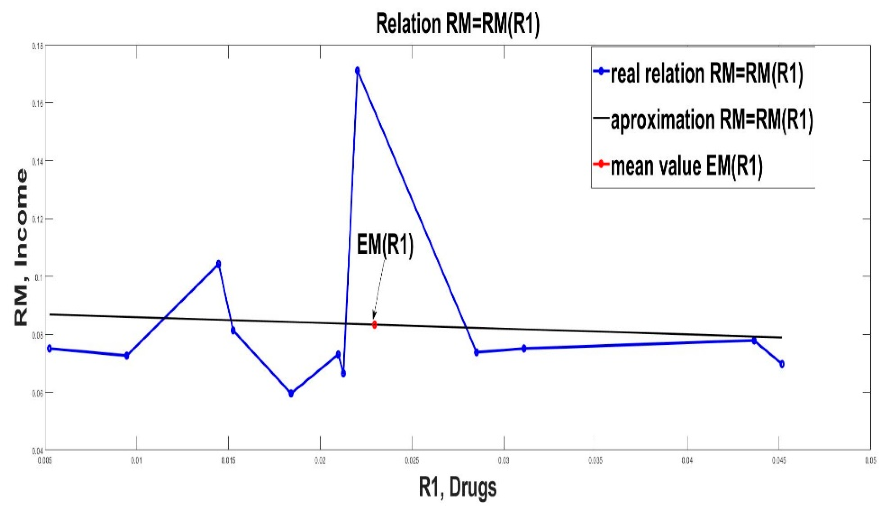
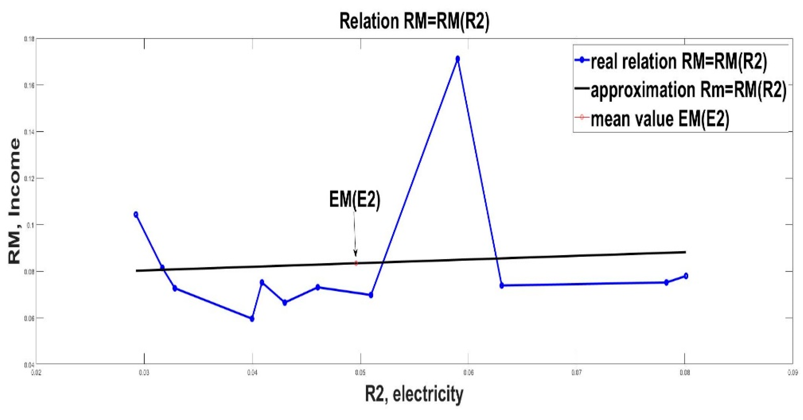
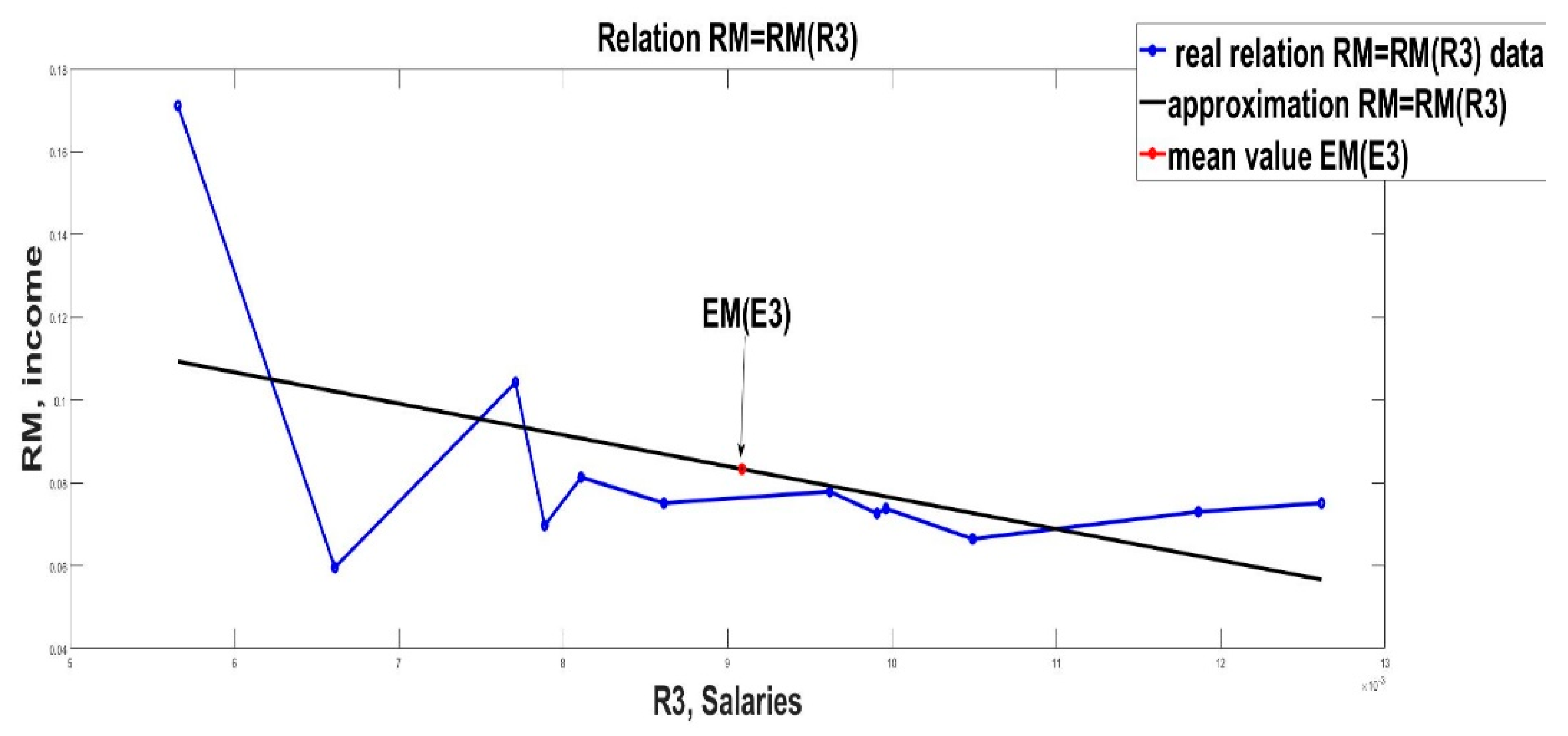
Graphical illustrations of the linear approximation (8) are given in Figure 2, Figure 3 and Figure 4.
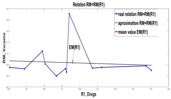
Figure 2.
Linear approximation of income RM from R1 (drugs).
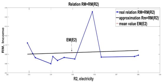
Figure 3.
Linear approximation of income RM from R1 (electricity).
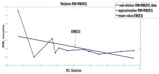
Figure 4.
Linear approximation of income RM from R3 (salaries).
5.7. Definition and Solution of Portfolio Problem (18)
Relation (13) for zero new investment resources is added as an additional constraint to the portfolio problem (18). The solutions to this portfolio problem are illustrated in Table 5.

Table 5.
Solutions of the portfolio problem (18) and constraint (13).
These results are interpreted according to the signs of the parameters bi, which is given in Table 5. For w4 and w5, the coefficients are b4 > 0 and b5 > 0, and the portfolio solutions recommend the disbursements of categories 4 and 5 to be increased by 85% and 0.2%, but the disbursement of category 10 must be decreased by 14% from its current value.
Without the portfolio solutions, the mean value of the income is . If the solutions of the portfolio problem are applied to increase or decrease the disbursements the income of the husbandry will be . Hence, the optimal management of the disbursements will increase the income with
These simulation results prove that the portfolio management of the disbursements can increase the mean husbandry income. The drawback of the algorithm comes from the sequence of usage of the initial portfolio data. For the definition of the parameters of the portfolio problem, the decision maker has to use available data for disbursements and income, but for the real case of business management, the real levels of the disbursements and income are not known currently, and they can be calculated hardly at the end of the management period. That is why in this research, we modify the algorithm above with the inclusion of a sliding procedure for active business management.
6. Active Business Management Applying the Derived Algorithm
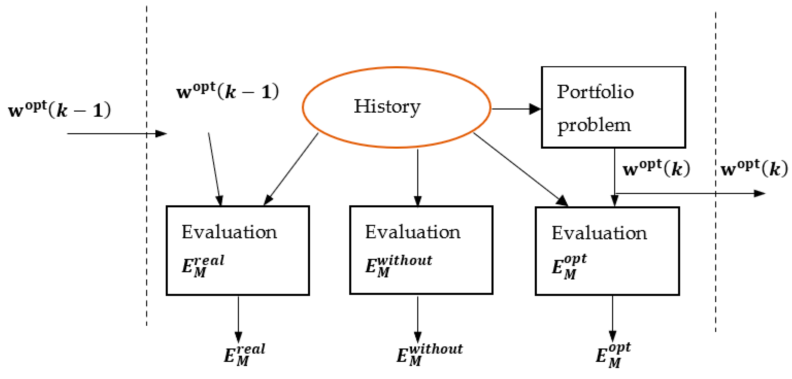
Active business management applies in a repeated way derived algorithm with different initial data. A window with a set of initial data is moving sequentially ahead for each step of management by definition and solving the appropriate portfolio problem. This rolling procedure is graphically illustrated in Figure 5.

Figure 5.
Rolling procedure for definition and solutions of portfolio problems.
For this research, the historical period for the data in the window is chosen for 3 months. These historical data are used for the definition and solution of a corresponding portfolio problem. The optimal solutions are applied for the next future period by correcting the disbursements and or providing recommendations for the future limitations of the mean disbursements per category. Thus, the business management will have reference data about the recommendations for the mean amount of disbursement per category by means to achieve the maximal level of income.
This active management procedure is assessed by calculating three types of income values:
- —For the management period k, it is used the available historical data. The recommendations from the previous period , which were evaluated by the portfolio problem, are applied by changing the current mean disbursements for the period k. The resulting income is evaluated. This is the real income found by the application of the portfolio problem.
- —This income is evaluated according to the current historical data. The resulting income is calculated without the application of portfolio optimization.
- —This is the optimal possible value of the income. It is evaluated according to the actual optimal weights , which are solved by the portfolio problem. This evaluation can be performed only at the end of period k, when the real mean values of disbursements should be available. This value gives the maximum income, which can be obtained if the weights were applied for business management for period k.
The evaluated are given as old values for the next k + 1 period and . The graphical interpretation of this active management is presented in Figure 6.
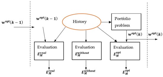
Figure 6.
Rolling active business management by changing the recommendations for mean levels of disbursements.
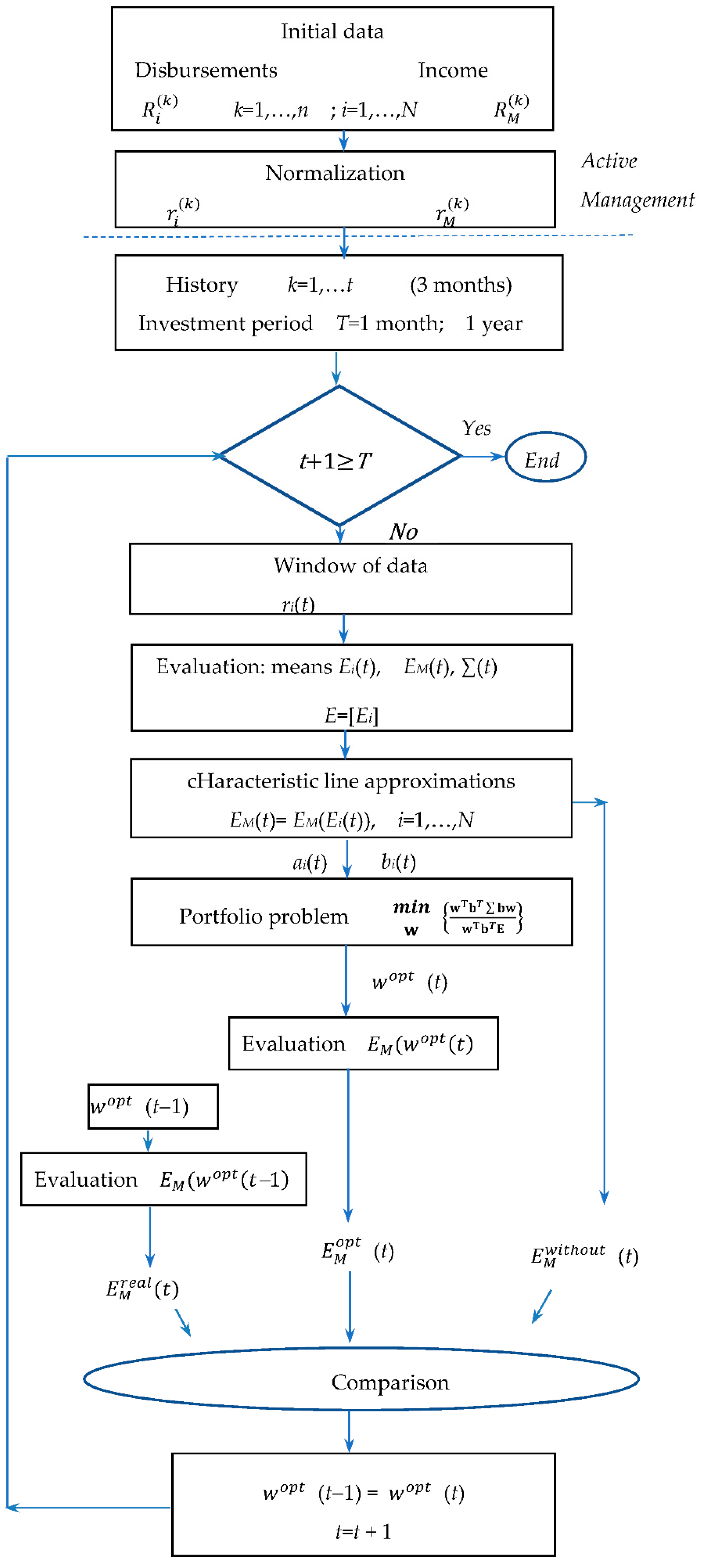
A flow chart of the operational rules of the algorithm is graphically interpreted in Figure 7. The initial data contain the monthly disbursements and income where k = 1, n is the period of available data, i = 1, N are the type of of disbursement. These sets of data are normalized to and by means of operating with fewer values of the data. For the active management, the historical period is chosen to be t = 1 year, and the investment period T is fixed to T = 3 years for Case1: 2019–2021, with results in Table 6. For Case 2, it takes t = 3 months history and T = 12 months (one year) with results in Table 7. According to the length and sequence of the widow, the corresponding initial data are taken from the set of normalized values and . The corresponding means of disbursements and income , , and covariance are calculated. Using these data, the corresponding characteristics lines are estimated by evaluation of the coefficients and , i = 1, N. They are used to evaluate the parameters for the portfolio problem (18) and constraints (13), where concerns the risk of the income increase, and is the mean value of the income increase. The solutions to the portfolio problem give recommendations on which type of disbursement to be increased (for ) and which to be decreased (for ). Then the comparison is made between the mean income for the defined period , the real achieved income, with the application of the evaluated weights from the previous period and the maximal potential case assuming precise forecast for the means values for the time window t. These three values are used as benchmarks for the evaluation of the benefit of the derived algorithm for the reallocation of resources between different types of disbursements.
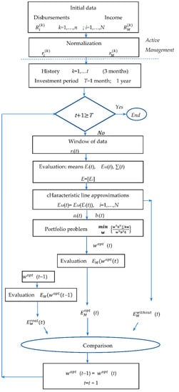
Figure 7.
Flow chart diagram of active business management.

Table 6.
Numerical results for the case of one-year historical period.

Table 7.
Comparisons between the income’s values with and without the application of active business management.
7. Empirical Simulations and Results
The amount of the historical period influences the solutions obtained by the portfolio problem. Respectively, the evaluated weights recommend the allocation of resources per disbursement for the mean values for the defined historical period. Here is the illustration of the results from the active management, applying different durations of the historical period.
7.1. Case 1: 2019–2021
The historical period is with duration of one year. The evaluated weights are applied for the next year as a management period. The graphical illustration of this active management is illustrated in Figure 8.

Figure 8.
Evaluation of the different categories of income for a historical period of one year.
The numerical results are summarized in Table 6.
These results demonstrate that the application of active business management gives income . The value of is calculated without the application of active management. The value of is the maximal potential income if actual weights have been applied, which will increase the real income or .
For illustration purposes, the evaluated weights per period k are given as follows. Only the nonzero values are denoted.
These results recommend for the next year 2020 the mean disbursements for E5 (credits) be decreased by 70% and increase the mean E10 (crops) by 29.66%.
These results recommend for 2021 the mean disbursements for E4 (insurance) increase by 43.96% and the mean disbursements for E10 (crops) decrease by 24.23%.
These recommendations are for 2022 again to increase the mean E4 (insurance) and to decrease the mean disbursements for E10 (crops) with the evaluated coefficients. Unfortunately, the real and optimal value of the income is not possible to evaluate in advance because the actual mean disbursements for 2022 are not available.
7.2. Case 2: 2021
For this case, the historical period is shortened to 3 months. The evaluated weights are applied one month ahead of the management period. In that case, the sequence of evaluation and sliding the management period is graphically presented in Figure 5. The initial historical period is for months 1–3 in 2021. The evaluated portfolio weights are applied for month 4. The corresponding incomes , , and are evaluated with and without the application of the weights are evaluated and compared. Then the active management makes a move for the historical period from months 2 till4. The newly evaluated weights are applied for month 5, and the corresponding values of the income are evaluated. For the 2021 year, such steps and sliding evaluations are k = 12 months − 3 months history = 9 steps. The results for the 2021 year are given in Table 7.
The increase in the mean real income towards the mean increase without the application of active management is
7.3. Case 3: 2019–2021
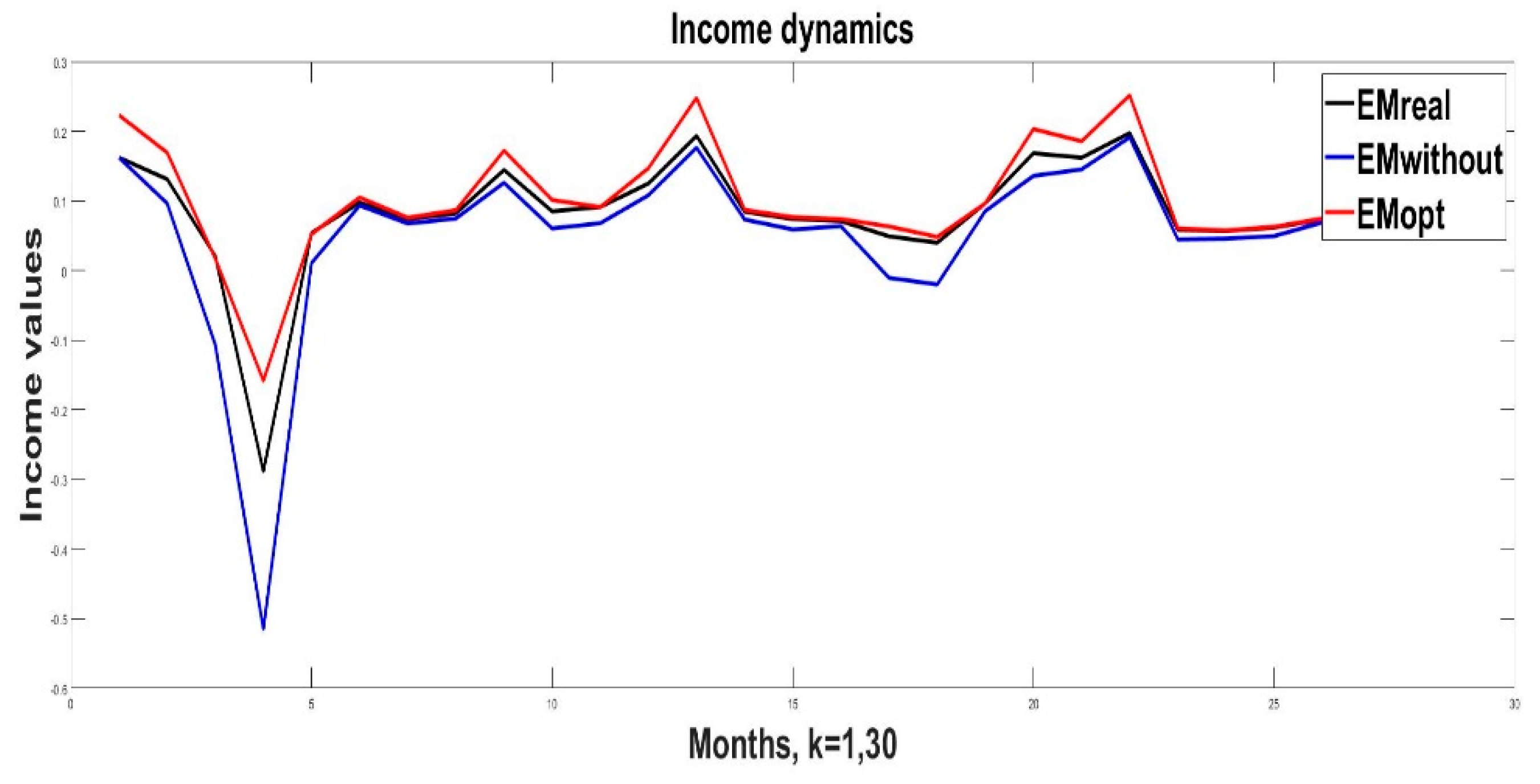
Here, the historical period is again 3 months. The application of the weights is for the next month, but the duration of the active management is for the entire period from 2019 to 2021. The behavior of the values of the three categories of incomes , , and are given in a graphical way in Figure 9.
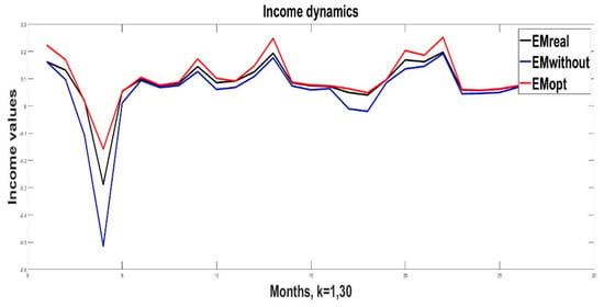
Figure 9.
The behavior of the three categories of income , , and .
To simplify the description and comparison of the resulting evaluations, here only the resulting mean values of the three categories of income are presented for the entire 3-year period.
It is seen again that the real mean income with application of the active management is bigger than the mean income without the application of the derived algorithm for recommending the levels of disbursements ≥ , but the value of a potential to increase till the level of . Even for this longer period of active management, the relations ≤ is kept. The increase in income, due to the application of the derived algorithm for active management, is
8. Discussion
The derived policy for active business management is based on the algorithm, which performs sequential definition and solution of portfolio problems. The obtained solutions are applied for the next future period (k + 1). Because in the future time the mean values of the disbursements will be different, the real mean income will differ, and it will be less than the potential optimal one . The solutions recommend a decrease or increase in corresponding disbursements according to the current levels of mean disbursements. The production technology of the business entity can insist limits on the resources that are needed; such constraints can be added to complicate the portfolio problem. This can be implemented simply by adding low and upper bounds to the values of disbursement in the portfolio problem or more complex mutual equalities or inequalities, but the algorithm does not estimate the future levels of such disbursements. Nevertheless, of the unknown values of the means Ei, the recommendations give an increase in the income when the means Ei are estimated at the end of the active future period k + 1. A potential exists by defining the portfolio problem with parameters, which are evaluated not only from the available data from the history of the disbursements but by the application of forecast approaches. Such approaches can be based on ARMA modeling (Auto-Regressive and Moving Average) [40], GARCH modeling (General Auto Regressive Conditional Heteroskedasticity) process [41], application of the Black–Litterman model for integration of historical data with expert subjective assessments about the future behavior of disbursements. Hence, a sequence of forecasting the levels of future means of disbursement can benefit the real obtained income , which should be closer to the potential optimal value . It is expected that such additional improvements and modifications of the derived algorithm will make less the difference between the real income and the potential maximal one for the used management period.
9. Conclusions
This research derives an algorithm that provides active management of the production policy of a business entity such as animal husbandry. The management is concerned with the appropriate redistribution of available resources between different types of disbursements. Thus, the income from production can increase without investing additional resources for production. The key component of this algorithm is the definition and solution of appropriate portfolio problems. Their solutions recommend the redistribution of resources between the different types of disbursements.
The numerical simulations illustrate that the application of the derived algorithm in the sequential application of the portfolio problem gives an increase in the husbandry income in comparison with the lack of such active business management. The numerical simulation has been performed with real data on animal husbandry from the region of Stara Zagora of Bulgaria. This active business management allows being automated the needed calculations by appropriate software suit. It has been discussed that the algorithm can be complicated with forecast modeling of the levels of disbursements, which will increase additionally the real husbandry income.
Author Contributions
Conceptualization, T.S.; methodology, T.S.; software, K.S.; validation, K.S.; formal analysis, T.S. and K.S. All authors have read and agreed to the published version of the manuscript.
Funding
This research was funded by Ministry of education and science of Bulgaria under the National Science Program INTELLIGENT ANIMAL HUSBANDRY, grant agreement N D01-62/18.03.2021.
Data Availability Statement
Bulgarian Science Program INTELLIGENT ANIMAL HUSBANDRY, grant agreement N D01-62/18.03.2021.
Conflicts of Interest
The authors declare no conflict of interest.
References
- Management Sciences. 2022. Available online: https://www.bing.com/search?q=management+sciences&cvid=99dcb5fc5e864436a573840efab06843&aqs=edge..69i57j0l8.4909j0j1&pglt=41&FORM=ANNTA1&PC=U531 (accessed on 17 October 2022).
- Taylor, F.W. The Principles of Scientific Management; Harper & Brothers: New York, NY, USA; London, UK, 1911. [Google Scholar]
- Vom Brocke, J.; Rosemann, M. Business Process Management. In Wiley Encyclopedia of Management; Wiley: Hoboken, NJ, USA, 2015. [Google Scholar]
- Rosemann, M.; vom Brocke, J. The Six Core Elements of Business Process Management. In Handbook on Business Process Management; Springer: Cham, Switzerland, 2010. [Google Scholar]
- Fundamentals of Business Management. Available online: https://blog.edx.org/6-fundamentals-of-business-management#:~:text=Fundamentals%20of%20Business%20Management%3A%20Explore%206%20Functional%20Areas,5.%20Data%20Analytics%20...%206%206.%20Marketing%20 (accessed on 17 October 2022).
- Business Functions. Available online: https://www.businessmanagementideas.com/business/functions-business/business-functions-7-main-types-of-business-function/3744 (accessed on 17 October 2022).
- Ngugi, D. Quantitative Methods for Business Management. 2018, p. 420. Available online: https://www.researchgate.net/publication/329031752_Quantitative_Methods_For_Business_Management (accessed on 17 October 2022).
- Fred, S.; Nassuna, A.; Byarugaba, P.; Arinaitwe, A. Quantitative Methods for Managerial Decision Making. 2020. Available online: https://www.researchgate.net/publication/340754384_quantitative_methods_for_managerial_decision_making (accessed on 17 October 2022).
- Alshater, M.M.; Saba, I.; Supriani, I.; Rabbani, M.R. Fintech in islamic finance literature: A review. Heliyon 2022, 8, e10385. [Google Scholar] [CrossRef] [PubMed]
- Soriano, R.R.; Budi, I.; Purwandari, B. Challenges and Trends of Financial Technology (Fintech): A Systematic Literature Review. Information 2020, 11, 590. [Google Scholar] [CrossRef]
- Sarhan, H. Fintech: An Overview; ResearchGate: Berlin, Germany, 2020; pp. 1–34. [Google Scholar] [CrossRef]
- Khotinskay, G.I. Fin Tech: Fundamental Theory and Empirical Features. In Proceedings of the Social and Behavioural Sciences GCPMED 2018 International Scientific Conference, 2019; Conference: GCPMED 2018—International Scientific Conference “Global Challenges and Prospects of the Modern Economic Development, Samara, Russia, 6–8 December 2018; pp. 222–229. Available online: https://www.researchgate.net/publication/331905682_Fin_Tech_Fundamental_Theory_And_Empirical_Features (accessed on 17 October 2022).
- Varga, D. Fintech, the new era of financial services. Vez. Bp. Manag. Rev. 2017, 48, 22–32. Available online: http://unipub.lib.uni-corvinus.hu/3170/1/VT_2017n11p22.pdf (accessed on 17 October 2022). [CrossRef]
- Kim, Y.; Choi, J.; Park, Y.; Yeon, J. The Adoption of Mobile Payment Services for “Fintech”. Int. J. Appl. Eng. Res. 2016, 11, 1058–1061. [Google Scholar]
- Yong, C.; Tham, J.; Azam, S.M.F.; Khatibi, A. Empirical study on acceptance of mobile payment and its competitive advantage in Malaysia. Eur. J. Soc. Sci. Stud. 2021, 7. [Google Scholar] [CrossRef]
- Markowitz, H. Portfolio selection. J. Financ. 1952, 7, 77–91. [Google Scholar]
- Sharpe, W. Portfolio Theory and Capital Market; McGraw Hill: London, UK, 2000; 316p. [Google Scholar]
- Black, F.; Litterman, R. Asset Allocation: Combining investor views with market equilibrium. J. Fixed Income 1991, 1, 7–18. [Google Scholar] [CrossRef]
- Satchell, S.; Scowcroft, A. A demystification of the Black–Litterman model: Managing quantitative and traditional portfolio construction. J. Asset Manag. 2000, 1, 138–150. [Google Scholar] [CrossRef]
- Meucci, A. The Black–Litterman approach: Original model and extensions. In The Encyclopedia of Quantitative Finance; Wiley: New York, NY, USA, 2010. [Google Scholar]
- Chen, J.M. On Exactitude in Financial Regulation: Value-at-Risk, Expected Shortfall, and Expectiles. Risks 2018, 6, 61. [Google Scholar] [CrossRef]
- Leung, M.; Wang, J.; Che, H. Cardinality-constrained portfolio selection via two-timescale duplex neurodynamic optimization. J. Neural Netw. 2022, 153, 399–410. [Google Scholar] [CrossRef]
- Dobrowolski, Z.; Drozdowski, G.; Panait, M.; Babczuk, A. Can the Economic Value Added Be Used as the Universal Financial Metric? Sustainability 2022, 14, 2967. [Google Scholar] [CrossRef]
- Sukharev, O.S. Portfolio Theory in Solving the Problem Structural Choice. J. Risk Financ. Manag. 2020, 13, 195. [Google Scholar] [CrossRef]
- Kato, Y. AI/Fintech and Asset Management Businesses. Policy Research Institute, Ministry of Finance, Japan. Public Policy Rev. 2020, 16, 1–28. [Google Scholar]
- Fagefors, C.; Lantz, B. Application of Portfolio Theory to Healthcare Capacity Management. Int. J. Environ. Res. Public Health 2021, 18, 659. [Google Scholar] [CrossRef]
- Lao, B.; Liu, N. Application of Portfolio Theory in Controlling Supply Chain Crisis. In Integration and Innovation Orient to E-Society 1; Wang, W., Ed.; IFIP International Federation for Information Processing, 251; Springer: Boston, MA, USA, 2007; pp. 9–16. Available online: https://link.springer.com/content/pdf/10.1007/978-0-387-75466-6_2.pdf (accessed on 17 October 2022).
- Cui, Y.; Cheng, C. Modern Portfolio Theory and Application in Australia. J. Econ. Bus. Manag. 2022, 10, 128–132. Available online: http://joebm.com/vol10/686-EM4270.pdf (accessed on 17 October 2022). [CrossRef]
- Barkley, A.; Peterson, H.H. Wheat Variety Selection: An Application of Portfolio Theory to Improve Returns. In Proceedings of the NCCC-134 Conference on Applied Commodity Price Analysis, Forecasting, and Market Risk Management, St. Louis, MO, USA, 21–22 April 2008. [Google Scholar]
- Hines, E. Application of Portfolio Theory to Commercial Real Estate. Johns Hopkins University, 2009. Available online: https://jscholarship.library.jhu.edu/bitstream/handle/1774.2/35837/Hines_Application%20of%20Portfolio%20Theory%20to%20Commercial%20Real%20Estate_2009_Gouline.pdf (accessed on 17 October 2022).
- Paut, R.; Sabatier, R.; Tchamitchian, M. Reducing risk through crop diversification: An application of portfolio theory to diversified horticultural systems. Agric. Syst. 2019, 168, 123–130. [Google Scholar] [CrossRef]
- Pulido-Rojano, A.; Pizarro-Rada, A.; Padilla-Polanco, M.; Sánchez-Jiménez, M.; De-la-Rosa, L.L. An optimization approach for inventory costs in probabilistic inventory models: A case study. Ing. Rev. Chil. Ing. 2020, 28, 383–395. [Google Scholar] [CrossRef]
- Mondal, R.; Shaikh, A.A.; Bhunia, A.K.; Hezam, I.M.; Chakrabortty, R.K. Impact of Trapezoidal Demand and Deteriorating Preventing Technology in an Inventory Model in Interval Uncertainty under Backlogging Situation. Mathematics 2022, 10, 78. [Google Scholar] [CrossRef]
- Chaiboonsri, C.; Wannapan, S. Multi-Process Analysis and Portfolio Optimization Based on Quantum Mechanics (QM) Under Risk Management in ASEAN Exchanges: A Case Study of Answering to the E-Commerce and E-Business Direction. In Handbook of Research on Innovation and Development of E-Commerce and E-Business in ASEAN; Almunawar, M.N., Ali, M.A., Lim, S.A., Eds.; IGI Global: Hershey, PA, USA, 2021; pp. 46–61. [Google Scholar] [CrossRef]
- Liu, X.; Luo, G.; Xu, X. Optimal Purchasing Decisions with Supplier Default in Portfolio Procurement. Mathematics 2022, 10, 3155. [Google Scholar] [CrossRef]
- Tang, M.-L.; Wu, T.-P.; Hung, M.-C. Optimal Pension Fund Management with Foreign Investment in a Stochastic Environment. Mathematics 2022, 10, 2468. [Google Scholar] [CrossRef]
- Standard Normal Distribution Showing Standard Deviations. Available online: https://www.statisticshowto.com/wp-content/uploads/2013/09/standard-normal-distribution.jpg (accessed on 17 October 2022).
- Kolm, P.N.; Tutuncu, R.; Fabozzi, F.J. 60 Years of portfolio optimization: Practical challenges and current trends. Eur. J. Oper. Res. 2014, 234, 356–371. [Google Scholar] [CrossRef]
- Kantar, Y.M. Generalized least squares and weighted least squares estimation methods for distributional parameters. REVSTAT Stat. J. 2015, 13, 263–282. [Google Scholar]
- Liu, C.; Shi, H.; Wu, L.; Guo, M. The Short-Term and Long-Term Trade-off between Risk and Return: Chaos vs Rationality. J. Bus. Econ. Manag. 2020, 21, 23–43. [Google Scholar] [CrossRef]
- Engle, R.F. Autoregressive Conditional Heteroscedasticity with Estimates of the Variance of United Kingdom Inflation. J. Econom. 1982, 50, 987–1007. [Google Scholar] [CrossRef]
Publisher’s Note: MDPI stays neutral with regard to jurisdictional claims in published maps and institutional affiliations. |
© 2022 by the authors. Licensee MDPI, Basel, Switzerland. This article is an open access article distributed under the terms and conditions of the Creative Commons Attribution (CC BY) license (https://creativecommons.org/licenses/by/4.0/).

