Article

Forecasting Day-Ahead Traffic Flow Using Functional Time Series Approach

1
Department of Statistics, Quaid-i-Azam University, Islamabad 45320, Pakistan
2
United Nations Industrial Development Organization, Islamabad 1051, Pakistan
3
Directorate of Sustainability and Environment, Capital University of Science and Technology, Islamabad 44000, Pakistan
4
Department of Mathematics, College of Sciences and Arts (Muhyil), King Khalid University, Muhyil 61421, Saudi Arabia
5
Department of Mathematics and Computer, College of Sciences, Ibb University, Ibb 70270, Yemen
6
Mathematics Department, Prince Sattam Bin Abdulaziz University, Al-Kharj 16278, Saudi Arabia
7
Department of Statistics and Information, Sana’a University, Sana’a 1247, Yemen
*
Author to whom correspondence should be addressed.
These authors contributed equally to this work.
Mathematics 2022, 10(22), 4279; https://doi.org/10.3390/math10224279
Submission received: 8 October 2022 / Revised: 10 November 2022 / Accepted: 12 November 2022 / Published: 16 November 2022

Abstract

:
Nowadays, short-term traffic flow forecasting has gained increasing attention from researchers due to traffic congestion in many large and medium-sized cities that pose a serious threat to sustainable urban development. To this end, this research examines the forecasting performance of functional time series modeling to forecast traffic flow in the ultra-short term. An appealing feature of the functional approach is that unlike other methods, it provides information over the whole day, and thus, forecasts can be obtained for any time within a day. Within this approach, a Functional AutoRegressive (FAR) model is used to forecast the next-day traffic flow. For empirical analysis, the traffic flow data of Dublin airport link road, Ireland, collected at a fifteen-minute interval from 1 January 2016 to 30 April 2017, are used. The first twelve months are used for model estimation, while the remaining four months are for the one-day-ahead out-of-sample forecast. For comparison purposes, a widely used model, namely AutoRegressive Integrated Moving Average (ARIMA), is also used to obtain the forecasts. Finally, the models’ performances are compared based on different accuracy statistics. The study results suggested that the functional time series model outperforms the traditional time series models. As the proposed method can produce traffic flow forecasts for the entire next day with satisfactory results, it can be used in decision making by transportation policymakers and city planners.

1. Introduction

The invention of vehicles has certainly made transportation easy, but it has also created multiple problems in today’s congested world, such as chronic, huge rush on a road at a time. This could lead to different issues, for example, accidents, delays for emergency travelers and wasting of precious time even for routine travelers. The accurate modeling and forecasting of traffic flow are crucial in today’s advanced world to get rid of such problems [1]. No one can subjectively predict the atypical conditions of traffic flow. Therefore, an accurate forecast could prevent people from facing major problems [2]. The United Nations Sustainable Development Goals (SDG) Agenda 2030 ties several goals to quality transportation and on-road mobility. There are a number of SDG targets directly related to transport, including SDG 3 on health (increased road safety), SDG 7 on energy, SDG 8 on decent work and economic growth, SDG 9 on resilient infrastructure, SDG 11 on sustainable cities (access to transport and expanded public transport), SDG 12 on sustainable consumption and production (ending fossil fuel subsidies) and SDG 14 on oceans, seas and marine resources (Sustainable Development Goals, UN knowledge platform, 2016). In addition, the accuracy of short-term traffic flow prediction as an indispensable measure is essential for the timely reporting of traffic conditions to the public and for the decision making of law enforcement to resolve traffic congestion [3].
A huge array of literature focuses on an intelligent transportation system to have better forecasting capability. Short-term traffic flow forecasting is essential for operations management and the dynamic scheduling of transport networks due to variations in traffic flow from hour to hour and day to day [4,5]. Most transportation management systems use short-term traffic flow forecasting techniques to undertake immediate decisions. In addition, these forecasts are helpful for policymakers to formulate policies accordingly for the future. Furthermore, accurate traffic flow forecasting can be very helpful for travelers to plan their travels accordingly. The realization of traffic control and guidance forms the core issue of an intelligent transportation system, and the real-time prediction of short-term traffic flow is a prerequisite for the scientific management and control of transport systems. Therefore, the real-time prediction of short-term traffic flow with accuracy is of enormous significance for effectively managing the traffic department and daily commuters [6].
In the past, different forecasting methods have been introduced in order to improve traffic flow forecasting accuracy [7]. Despite massive investments in transportation-related infrastructure, traffic congestion remains a societal and public policy problem of paramount importance. Intelligent transportation systems (ITS) have been potentially proposed as a solution to this issue, but their effectiveness remains vague in research and applied practices. Ref. [8] stated that “ITS helps individual commuters to make better travel decisions, and it helps local governments to develop an urban traffic management capability”. Their study concluded that there is significant empirical evidence that supports the underlying theories and shows that ITS helps commuters to schedule and sequence travel more efficiently, opt for appropriate navigation routes, and optimize their work trip transportation mode. Secondly, the social impact of ITS is highly dependent upon the available road network and the widely accessible public transit services.
The main aim of this research is to propose an efficient model for forecasting a day-ahead traffic flow based on functional time series modeling. An appealing feature of the functional approach is that unlike other methods, it provides information over the whole day, and thus, forecasts can be obtained for any time within a day. In this study, a functional datum is referred to the day profile of traffic flow collected at some discretized points. Considering the day profile as a single functional datum solves the problem of high dimension and enables use of the correlation among values within a functional datum. The proposed model performs better on weekdays as well as on weekends. The forecasting accuracy of the functional model is compared with the classical ARIMA models that are frequently used in the literature for traffic flow forecasting.
The remaining article is organized as follows. Section 2 provides a literature review concerning traffic flow forecasting. The methods and models used in this study are given in Section 3. Section 4 presents an empirical investigation of the model’s performance on a real data set, while Section 5 provides the conclusion and future recommendations.

2. Literature Review

In recent decades, researchers have proposed a variety of short-term traffic forecasting models differing in complexity, methodology, and performances [9,10,11,12,13]. The researchers used different traffic flow parameters to propose efficient models in different scenarios. For example, ref. [14] compared three different models, i.e., the random walk model, Holt–Winter’s exponential smoothing model, and the Seasonal AutoRegressive Integrated Moving Average (SARIMA) model for forecasting traffic flow. Holt–Winter’s exponential smoothing model was declared the best, while the SARIMA was competitive. Ref. [15] used the functional principle components analysis technique to develop high-quality internet traffic volume projections. It was found that the functional principal components analysis increases the forecasting ability. Ref. [16] used functional clustering to know the traffic flow pattern. The functional mixture prediction approach used by [17] was found to be better than the functional principal components approach. Ref. [18] implemented a functional nonparametric kernel regression model to forecast the traffic flow. Ref. [19] used the Generalized AutoRegressive Conditional Heteroskedasticity (GARCH) model for forecasting traffic flow. Ref. [20] considered the long-range temporal dependence and daily temporal dependence for modeling the traffic flow time series and suggested that both the dependencies are equally important and should be considered simultaneously.
A hybrid model for short-term traffic flow forecasting was proposed by [21] which combines ARIMA and the support vector machine (SVM) technique. Ref. [22] introduced a hybrid model namely dynamic spatio-temporal ARIMA for short-term traffic flow forecasting. Ref. [23] analyzed the correlation between the long short-term memory network (LSTM) and the statistical characteristics of the traffic flow data to modify a long short-term memory network model. The logistic regression model and ARIMA model were compared by [24]. The study suggested that ARIMA produced better results than the logistic model. Ref. [25] proposed a model which overcomes the memoryless property of the previous nonparametric method. Ref. [26] compared four regression models for traffic flow forecasting: sequential minimal optimization (SMO) regression, linear regression, multilayer perceptron, M5P model tree, and random forest. Ref. [4] proposed a novel method for forecasting combining the framework of the heaped auto-encoder and radial basis function neural network. Ref. [27] developed a hierarchical linear vector AutoRegressive model to know the spatio-temporal relations of the traffic flow. Ref. [28] constructed a prediction network to forecast traffic flow, i.e., long short-term memory, based on a deep learning algorithm. An adaptive hybrid model that combines linear ARIMA and nonlinear wavelet neural network to predict short-term traffic flow was proposed by [29]. Ref. [30] compared the forecasting performance of gradient boosting decision tree and wavelet neural network to propose a better model for traffic flow forecasting. Ref. [31] presented a combined deep learning model for short-term traffic flow forecasting based on LSTM, Gater Recurrent Unit (GRU), Convolution Neural Network (CNN), and Dynamic Optimal Weighted Coefficient Algorithm (DOWCA).
For short-term traffic flow forecasting, the proposed model by [32] decomposes data into three modeling components, i.e., periodic trend by introducing spectral analysis technique, the volatility estimated by the GRU-GARCH model, and a deterministic part modeled by the ARIMA model. Ref. [33] presented a hybrid Particle Swarm Optimization (PSO)-SVR method for short-term traffic flow forecasting. A PSO-ELM (Extreme Learning Machine) model based on particle swarm optimization for short-term traffic flow forecasting was proposed by [34]. The model was capable of controlling the nonlinear relationship effect that could result in lower forecast accuracy. Ref. [35] compared the forecasting performance of a nonparametric K-Nearest Neighbor (KNN)-based regression model with a neural network. The KNN method was more effective than the neural network, which had the advantage of strong transplant ability compared to the neural network. Ref. [36] proposed a hybrid model for short-term traffic flow forecasting by combining a deep polynomial neural network and SARIMA model. In addition, researchers also compared statistical models with artificial intelligence models. For example, ref. [37] compared ARIMA, neural network, and nonparametric regression models. Nonparametric regression performed better when traffic flow fluctuates quickly. However, it was concluded that all the models perform equally when traffic flow does not fluctuate quickly. Ref. [38] analyzed statistical methods for short-term traffic flow forecasting. The methods include average history methods, ARIMA, SARIMA, space-time ARIMA, nonparametric methods, neural networks, support vector machine, and hybrid models. The hybrid techniques were declared the best among these models. Ref. [15] proposed a novel compound model for short-term traffic flow forecasting in the presence of both typical and atypical traffic flow conditions. Ref. [39] compared the proposed model “ S V R R B F s ” with several statistical and artificial intelligence-based models. Ref. [40] compared different statistical and artificial intelligence-based models, such as historical average, back-propagation neural network, time series and nonparametric regression. The nonparametric regression model was the best among the three models. Ref. [41] considered three models for forecasting the traffic flow of major urban areas. Among the three models, the neural network model was more effective.

3. Methods and Models

The main goal of this study is to forecast a day-ahead traffic flow by using a functional time series model. For this purpose, a Functional Autoregressive (FAR) is used for forecasting a day-ahead traffic flow. The functional model FAR is compared with the popular ARIMA(p,d,q). Before going into details of the models mentioned above, a brief introduction to the functional data analysis is given below.

3.1. Functional Data Analysis

Functional data analysis (FDA) is a group of methods analyzing data over a curve, surface, or continuum. FDA considers each curve as a single observation instead of a collection of discrete data points [42,43,44]. In FDA, the data collected at discretized points, often equally spaced, are converted to functional data by implementing a suitable basis functions system. The functional data are then represented in the form of curves. The basis functions have the ability to eliminate the common noise and represent each data curve that resembles the original data by means of smoothing. A basis functions system is defined as a set of functions that is a linear combination of the coefficients c k and basis functions ϕ k . The linear combination of coefficient c k and ϕ k explains the functional observations. For example, a functional observation x ( t ) is defined as
x ( t ) = k = 1 K c k ϕ k ( t ) ,
where c k are parameters (coefficients) and ϕ k are known basis functions. Here, K denotes the number of basis functions used in the basis function system that is generally computed by the cross-validation technique. Different basis functions are available that can capture the underlying process more efficiently. For periodic data, Fourier basis functions are generally used. Fourier basis are a linear combination of sine and cosine functions of increasing frequency. Mathematically, the Fourier basis can be written as
x ^ ( t ) = c 0 + c 1 sin ω t + c 2 cos ω t + c 3 sin 2 ω t + c 4 cos 2 ω t + .
Here, c 0 = 1 is a constant, and c 1 , c 2 ,…, c k are the coefficients of K basis functions. In addition, K will always be odd number because of one constant. The ω defines the period 2 π / ω .

3.2. Functional Autoregressive Model

Functional data analysis is a modern and relatively less explored field for forecasting traffic flow, where analysis is performed by using the traffic flow information over an entire day. In this research, the FAR model is used, which is an extension of the autoregressive model but in the functional context. The time series values are formed functionally via discretized points representing discrete data collected at some intervals of a day. Mathematically, the FAR(1) model is given as:
Y t j = ψ Y t 1 j + ϵ t ( j ) .
Here, Y t j and ϵ t ( j ) are curves evaluated at j discretized points, and ψ is an operator called a projector (parameter). The ϵ t ( j ) is a random error, such that ϵ t ( j ) is normally distributed with mean zero and variance σ ϵ 2 ( j ) . The Y t ( j ) is an observed functional datum which is assumed a causal process for any j [45]. The estimation of autoregressive operator of the FAR(1) model can be estimated under the conditions that there exists an integer j 0 0 such that ψ j 0 < 1 and the process { Y t } satisfies E Y 0 4 < . The first condition is denoted by C 0 , while the second condition is denoted by C 1 . To understand the estimation of the FAR(1) model, first consider the traditional AR(1) model given as
Y t = ψ Y t 1 + ϵ t .
In this model, all the quantities are scalars. It is assumed that | ψ | < 1 , which indicates the process is stationary. AR(1) is multiplied by Y t 1 followed by taking expectation on both sides that results, γ 1 = ψ γ 0 . Similarly, γ k = E[ Y t , Y t + k ] is defined. The γ k autocovariance is estimated by γ k ^ which denotes the sample autocovariance. Finally, the estimator of ψ is ψ ^ = γ ^ 1 / γ ^ 0 . This technique is extended to the functional time series model to estimate FAR(1) model [46] as follows.
E Y t , y Y t 1 = E ψ ( Y t 1 ) , y Y t 1 .
Now, the lag 1 autocovariance operator is defined by,
C 1 ( y ) = E Y t , y Y t + 1 .
It is denoted by the adjoint operator, i.e., superscript · T . Then, C 1 T = C ψ T because it is already known that C 1 T = E Y t , y Y t + 1 , i.e.,
C 1 = ψ C
Since Equation (4) is similar to the scalar case, the estimate of ψ can be obtained by implementing a finite sample version of the relation ψ = C 1 C 1 . Since the operator C has no bounded inverse on the H (Hilbert-space), which means that C 1 ( C ( y ) ) = y , where
C 1 ( x ) = j = 1 λ j 1 x , ν j ν j .
The operator C 1 can be defined if all λ j are positive. If λ 1 λ 2 λ p > λ p + 1 = 0 , then { Y t } is in the space spanned by { ν 1 , , ν p } . The C 1 can be defined by C 1 ( x ) = j = 1 p λ j 1 x , ν i ν i on the subspace. The ‖ C 1 ‖ = λ t 1 , as t tends to , so, it is unbounded. This scenario makes it burdensome to estimate the bounded operator Ψ using the relation Ψ = C 1 C 1 . The solution to this problem is to utilize the first p most important empirical functional principal components (EFPC’s) ν ^ j . Thus,
I C ^ p ( y ) = j = 1 p λ ^ j 1 y , ν ^ j ν ^ j .
The operator I C ^ p is defined on the whole space L 2 . This operator will be bounded if λ ^ j > 0 for j p . The p components are chosen in such a way that the balance between maintaining the admissible information contained in the sample and the risk of dealing with reciprocals of small eigenvalues λ ^ j . For a computable estimator of Ψ , an empirical version of Equation (4) is used. It is known that C 1 is estimated as,
C ^ 1 ( y ) = 1 N 1 k = 1 N 1 Y k , y Y k + 1 ,
so, the following form is obtained, for any y L 2 ,
C ^ 1 I C ^ p ( y ) = C ^ 1 j = 1 p λ ^ j 1 y , ν ^ j ν ^ j = 1 N 1 k = 1 N 1 Y k , j = 1 p λ ^ j 1 y , ν ^ j ν ^ j Y k + 1 = 1 N 1 k = 1 N 1 j = 1 p λ ^ j 1 y , ν ^ j Y k , ν ^ j Y k + 1 .
This estimator can be implemented, but commonly, an additional smoothing step is introduced by utilizing the approximation Y k + 1 i = 1 p Y k + 1 , ν ^ i ν ^ i . This leads to the estimator,
Ψ ^ ( y ) = 1 N 1 k = 1 N 1 j = 1 p i = 1 p λ ^ j 1 y , ν ^ j Y k , ν ^ j Y k + 1 , ν ^ i ν ^ i .
The estimator in Equation (5) is a kernel operator with kernel,
ψ ^ p ( t , s ) = 1 N 1 k = 1 N 1 j = 1 p i = 1 p λ ^ j 1 Y k , ν ^ j Y k + 1 , ν ^ i ν ^ j ( s ) ν ^ i ( t ) .
This is verified by noting that,
Ψ ^ p ( y ) ( t ) = ψ ^ p ( t , s ) y ( s ) d s .
Since ψ (·,·) is a Hilbert–Schmidt kernel, then
ψ ^ p ( t , s ) = i , j = 1 p ψ ^ i j ν ^ i ( t ) ν ^ j ( s ) ,
where ψ ^ i j = ψ ^ ( t , s ) ν ^ i ( t ) ν ^ j ( s ) d t d s . Therefore,
ψ ^ p ( t , s ) Y k ( s ) d s = i , j = 1 p ψ ^ i j ν ^ i ( t ) Y k , ν ^ j .
For any 1 ≤ ip, we have
Y k + 1 , i = j = 1 p ψ ^ i j ξ k j + e k + 1 , i + η k + 1 , i
where
Y k + 1 , i = Y k + 1 , i , ξ k j = Y k , ν ^ j , e k + 1 , i = ϵ k + 1 , ν ^ i
a n d η k + 1 , i = j = 1 p ψ ^ i j Y k , ν ^ j .
The errors e k + 1 , i and η k + 1 , i are combined,
σ k + 1 , i = e k + 1 , i + η k + 1 , i .
It is to be noted that σ k + 1 , i are no longer IID. Now,
Y k = [ ξ k 1 , , ξ k p ] T , Y k + 1 = [ Y k + 1 ( 1 ) , , Y k + 1 ( p ) ] T , σ k + 1 = [ σ k + 1 ( 1 ) , , σ k + 1 ( p ) ] T ,
ψ ^ = [ ψ 11 , , ψ 1 p , ψ 21 , , ψ 2 p , ψ p 1 , , ψ p p ] T
Equation (6) can be rewritten as,
Y k + 1 = Z k ψ ^ + σ k + 1 , k + 1 = 1 , 2 , , N k = 1 , 2 , , N
where each Z k is a p × p 2 matrix,
Z k = Y k T 0 p T . . . 0 p T 0 p T Y k T . . . 0 p T 0 p T 0 p T . . . Y k T
with 0 p = [ 0 , , 0 ] T . Finally, the Np × 1 vectors Y, σ and the Np × p 2 matrix Z are defined as,
Y = Y 1 Y 2 Y N σ = σ 1 σ 2 σ N Z = Z 1 Z 2 Z N
As a result, the following linear model is obtained,
Y = Z ψ ^ + σ .
It is worth noting that Equation (7) is not a traditional linear model. First of all, the design matrix Z is random. Secondly, Z and σ are not independent. The error term σ is the combination of ϵ (projections of the error term) and η . Thus, Equation (7) looks like a linear model, but the current asymptotic results do not apply to it. A new asymptotic analysis involving the interaction of the various approximation errors is needed. Equation (7) leads to the formal least squares estimator for Ψ as follows [46],
ψ ^ = ( Z ^ T Z ^ ) 1 Z ^ T Y ^

3.3. Autoegressive Integrated Moving Average (ARIMA) Model

ARIMA models are one of the most popular and frequently used forecasting models to model and forecast traffic flow. An ARIMA model is a combination of three components: AR(p), I(d), and MA(q). The choice of the values of p,d, and q is very important, and the Box and Jenkins methodology is generally used to select them. When a time series is nonstationary, it is differentiated (d times) to convert it to stationary series. In ARIMA(p,d,q), the AR(p) denotes p lagged values of a time series, I(d) denotes the order of differencing, and MA(q) term represents the number of lags error terms included in the model. Mathematically, an ARIMA(p,d,q) can be written as
Y t d = β 0 + r = 1 p φ r Y t r d + i = 1 q Φ i ϵ t i + ϵ t
where Y t d represents the dth difference of series, and φ r ( r = 1 , 2 , , p ) and Φ i ( i = 1 , 2 , , q ) are the parameters of AR and MA terms, respectively. Moreover, ϵ t is an error term such that ϵ t ∼ N(0, σ ϵ 2 ). The values for p, d, and q are selected by inspecting the autocorrelation (ACF) and partial autocorrelation (PACF) plots of the series. Once the model parameters are identified, they can be estimated using the maximum likelihood estimation (MLE) method. A flowchart of the proposed modeling framework is presented in Figure 1.

4. Analysis and Results

This section contains a description of the data, provides results, and discusses the important findings of the research.

4.1. Data Description

Taking advantage of technology, nowadays, traffic flow data are gathered with the help of scanners. With the availability of massive data, researchers are trying to improve the forecasting accuracy of different modeling techniques. In this research, the traffic flow data of a busy highway (airport road) in Dublin, Ireland, have been used. In particular, the data were collected at M01 Airport Link Road between R132 Swords Road and Jn2 Dublin Airport. This airport link road is one of the busiest roads and remains very busy throughout the day. People used this road to access the airport as well as their workplaces. The data are freely available from the TII Traffic Data website (https://trafficdata.tii.ie, accessed on 11 October 2021). For empirical analysis, the data from 1 January 2016 to 30 April 2017 were obtained at each 15-min interval, leading to 96 data points for a single day. The data were divided into two sets, i.e., the first twelve months are used as a model estimation period, and the last four months are used for the one-day-ahead out-of-sample forecast. The main reason to use a larger window for the out-of-sample forecast is to assess the forecasting performance of different models in different situations. An example of the traffic flow data set collected at the Dublin airport link road for different days of a week and different periods of a day is given in Table 1.

4.2. Discrete Noisy Data Conversion to Functional Data

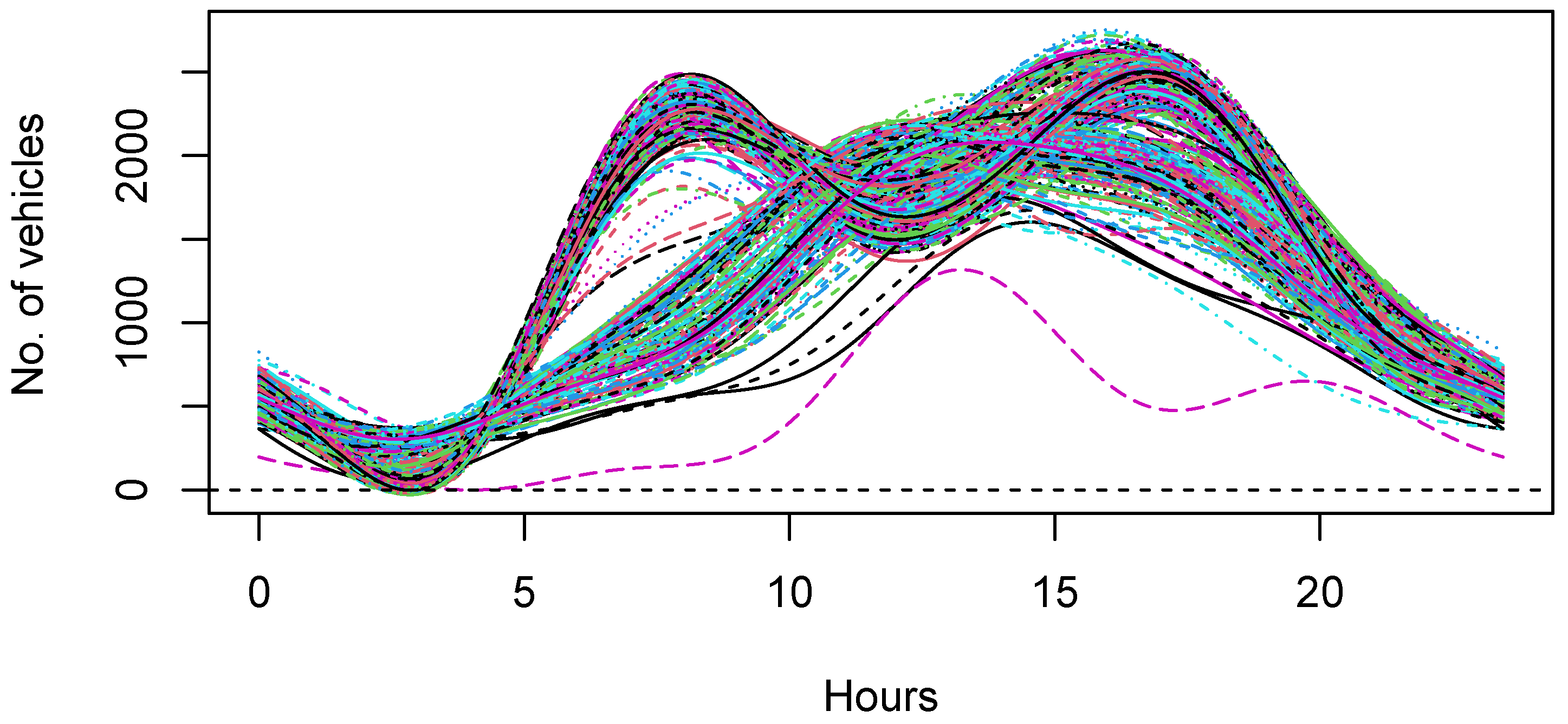
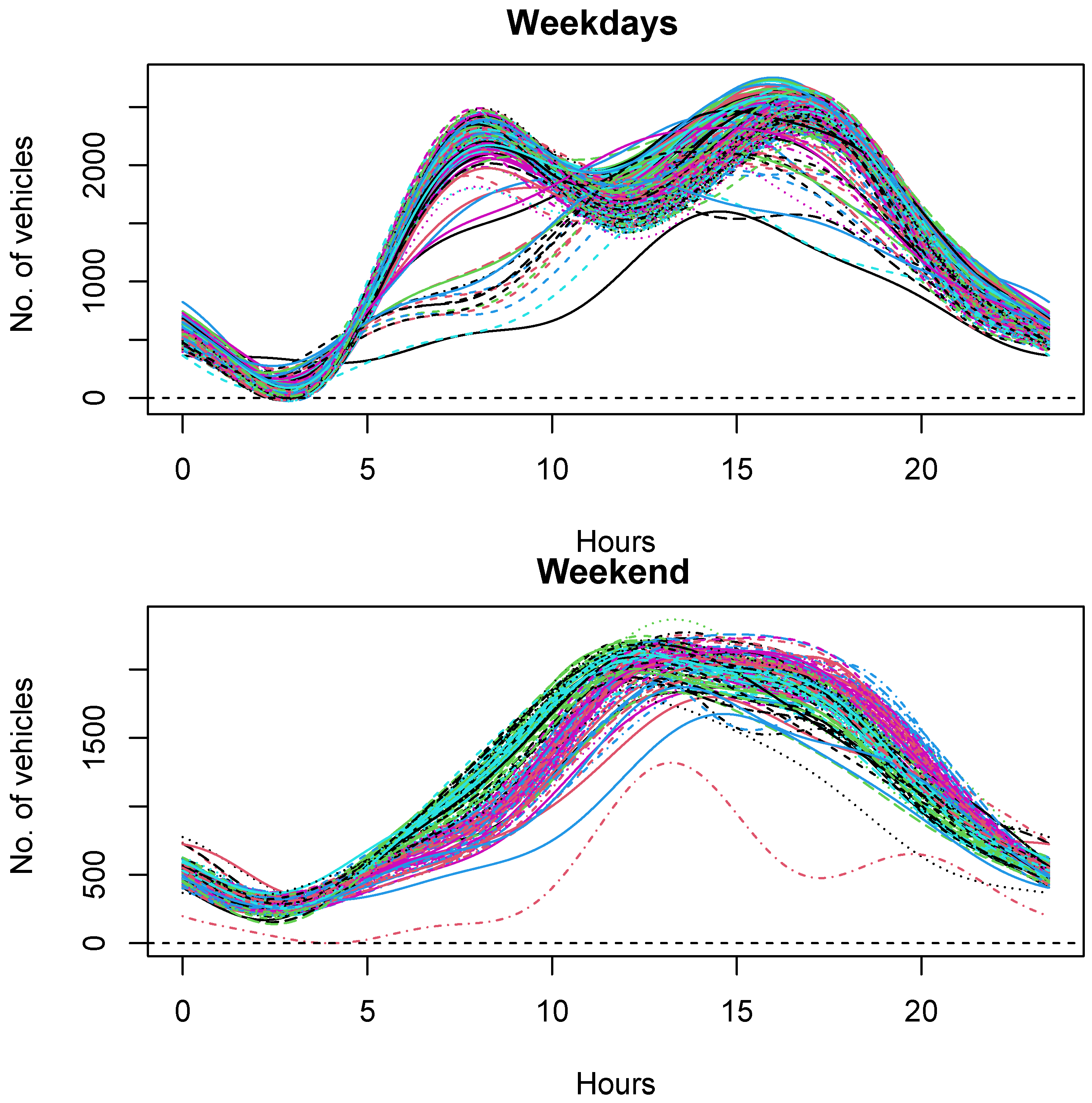
The first step of the analysis involved the conversion of the discrete noisy data to smooth functions. The daily traffic flow profile consists of 96 discrete points corresponding to a 15-min interval collected data. As the data were periodic, we used the Fourier basis. Using the Fourier basis functions, the raw data were converted to functional data by implementing nine basis functions. For illustration, Figure 2 provides the smoothed daily profile for the data used in this study. From the figure, it is evident that there are two patterns of traffic flow corresponding to working days and weekend days. To account for weekly periodicity, the traffic flow data are separated into two datasets, i.e., working days and weekends. Both the raw data are converted into functional data using the aforementioned method. The polts of both data sets are depicted in Figure 3. It is noticed from the plot that there is a substantial difference in traffic flow between working days and weekend days. Concerning the working day’s pattern, the traffic flow has its first peak in the morning time as people go to their workplaces and educational institutes. The traffic flow gradually decreases in the afternoon time and then again increases around 3:00–4:00 PM as people return from educational institutes and workplaces. As the data are from the airport link road, it is also possible that most air travels are scheduled around these times. In contrast, the weekend traffic flow is significantly different from working days. The weekend traffic flow is a bit high in the afternoon because of the airport route. Although both patterns are very consistent, however, some days behave a bit differently as compared to their general patterns. It might be because of some exceptional holidays such as bank holidays, festival holidays, etc.

4.3. Models Estimation

The main aim of the article is to model and forecast one-day-ahead traffic flow. To this end, the models are applied to the data in two different scenarios: (i) when ignoring the weekly periodicity, i.e., the models are directly applied to the whole data, and (ii) when considering the weekly periodicity, i.e., in this case, the models are applied to weekday data and weekend data separately. Note that in both cases, the parameter values of the models are different. The FAR(1) model is applied in both cases separately in the functional modeling approach.
On the other hand, ARIMA model parameters were identified by analyzing the ACF and PACF plots of the series. A restricted ARIMA(7,1,0) model where lag = 3 , 4 , 5 , and 6 equal to zero due to their insignificance is found to be the best fitted model for the combined data set. In case two, the best model for working days is a restricted ARIMA(5,1,0) with lag = 3 and 4 equal to zero, as they were insignificant. For the weekend, the ARIMA(2,1,0) is found to be the best model and fitted to the data. Mathematically, these models are given as
Y t 1 = β 0 + φ 1 Y t 1 1 + φ 2 Y t 2 1 + φ 7 Y t 7 1 + ϵ t
Y t 1 = β 0 + φ 1 Y t 1 1 + φ 2 Y t 2 1 + φ 5 Y t 5 1 + ϵ t
Y t 1 = β 0 + φ 1 Y t 1 1 + φ 2 Y t 2 1 + ϵ t
where Y t 1 denotes the integrated series. The φ i is the associate coefficient to the lag and ϵ t is the error term.

4.4. Out-of-Sample Forecasting

The models are trained using the first twelve months, and the last four months are used for one-day-ahead out-of-sample forecasting. Both models are used to forecast a day-ahead traffic flow in both data cases. The models’ performance is assessed by four different accuracy statistics, including mean square error (MSE), mean absolute error (MAE), mean absolute percentage error (MAPE), and mean squared percentage error (MSPE). In addition, day-specific mean absolute percentage error (DS-MAPE) is also calculated to assess the forecasting performance of different models on different days of a week. Mathematically, these accuracy measures can be written as
MSE = 1 t j Y t , j Y ^ t , j 2 MAE = 1 t j | Y t , j Y ^ t , j | MAPE = 1 t j | Y t , j Y ^ t , j | Y t , j × 100 MSPE = 1 t j | Y t , j Y ^ t , j | Y t , j 2 × 100 DS - MAPE d a y = 1 t j | Y t , j Y ^ t , j | t d a y , j Y t , j × 100
where Y t , j and Y ^ t , j are the observed and forecasted traffic flow for the tth day ( t = 1 , 2 , , 120 ) and jth time-period ( j = 1 , 2 , , 96 ), respectively. Meanwhile, t  day, j, denotes specific days (Monday,⋯, Sunday).
The accuracy results concerning the one-day-ahead out-of-sample forecast using the functional and traditional models are given in Table 2.
From the table, it is evident that our proposed functional model performs relatively better than ARIMA models. For example, when working with the complete data set, the MAPE value of the restricted ARIMA(7,1,0) model is 1.86% higher than the MAPE of FAR(1), which is a significant difference. In this case, FAR(1) produces the values for MSE, MAE, MAPE, and MSPE of 24762.96, 102.01, 9.94, and 2.75, respectively, whereas these values for ARIMA(7,1,0) are 38871.68, 118.13, 11.80, and 3.90. On the other hand, the accuracy statistics of the restricted ARIMA(5,1,0) model are higher than the FAR(1) model when considering data only corresponding to the working days. In this case, the MAPE value of the FAR(1) model is 8.24, which is considerably lower than the MAPE value obtained with restricted ARIMA(5,1,0). The MAPE value of the restricted ARIMA(5,1,0) exceeds 1.17% of the MAPE of FAR(1). In the case of considering only weekend days data, all the accuracy statistics of FAR(1) are lower than the ARIMA(2,1,0), which indicates the superiority of the FAR(1) model. The MAPE value of 10.30 obtained by the ARIMA(2,1,0) is slightly higher than the MAPE value of 9.36 obtained by the FAR(1). It is worth mentioning that in all the cases, the proposed FAR model outperforms the competitors as the accuracy statistics values are considerably lower for FAR than ARIMA. For illustration purposes, the MAPE values are also depicted in Figure 4. This figure clearly shows that the FAR model produces lower MAPE values than the competitors.
The accuracy results can be differentiated by looking at graphs in the above figure. The day-specific MAPE (DS-MAPE) values for different models are listed in Table 3. Again, the functional model can be easily compared with the traditional model in terms of forecasting accuracy for the traffic flow on different days of the week. The MAPE values for the FAR(1) model are comparatively lower than those of the ARIMA models. The lowest MAPE values are obtained on Thursday, while Monday produces higher MAPE values. The DS-MAPE values are also depicted graphically in Figure 5. In Figure 5, it can be seen that the FAR(1) model performs relatively better than ARIMA models comparing the traffic flow forecast on specific days.

5. Conclusions and Recommendations

The functional data analysis approach is a modern and less explored field for modeling and forecasting short-term traffic flow. This paper proposes a functional time series model to forecast a day-ahead traffic flow. In particular, this research work utilized a functional autoregressive model and compared it with the most frequently used classical time series models, ARIMA. The traffic flow data of Dublin airport link road is used to assess the forecasting performance of the functional model and the traditional time series models.The data set ranges over 16 months, collected at every 15-min interval, thus leading to 46,956 data points. The first twelve months are used for model estimation, whereas the last four months are used for one-day-ahead out-of-sample forecasts. The forecasting accuracy of models is measured by four different accuracy measures, namely, RMSE, MAE, MAPE, and MSPE. Finally, the models are applied to the complete data set as well as by splitting the data into weekdays and weekends to account for the weekly periodicity.
The results provided by the accuracy statistics suggest that the functional model outperforms the traditional models in all cases. The FAR(1) model produces significantly lower forecasting errors than the ARIMA models used in the study. The day-specific MAPE suggests that the errors vary over the whole week, with a high observed on Monday and Thursday producing lower errors. In addition, an appealing feature of the functional approach is that unlike other methods, it provides information over the whole day, and thus, forecasts can be obtained for any time within a day. As the proposed method can produce traffic flow forecasts for the entire next day with satisfactory results, it can be used in decision making by transportation policymakers and city planners. In the future, other exogenous information, such as weather information, unforeseen disruptions, etc., can be used in the functional model to evaluate its significance on the forecasting results. In addition, machine learning models’ performance can be compared with functional models.

Author Contributions

Conceptualization, I.S.; Software, S.A. (Saira Ahmed) and M.M.A.A.; Formal analysis, I.M. and S.A. (Saira Ahmed); Investigation, I.M. and S.A. (Sajid Ali); Resources, S.A. (Sajid Ali) and A.Y.A.-R.; Writing—original draft, I.M. and S.A. (Sajid Ali); Writing—review and editing, I.S., S.A. (Saira Ahmed), M.M.A.A. and A.Y.A.-R.; Supervision, I.S.; Funding acquisition, I.S., M.M.A.A. and A.Y.A.-R. All authors have read and agreed to the published version of the manuscript.

Funding

This research was funded by scientific research at King Khalid University through larg groups (project under grant number RGP.2/4/43).

Institutional Review Board Statement

Not applicable.

Informed Consent Statement

Not applicable.

Data Availability Statement

Not applicable.

Acknowledgments

The authors extend their appreciation to the Deanship of Scientific Research at King Khalid University for funding this work through Larg Groups (project under grant number RGP.2/4/43).

Conflicts of Interest

The authors declare no conflict of interest.

References

  1. Vlahogianni, E.I.; Karlaftis, M.G.; Golias, J.C. Short-term traffic forecasting: Where we are and where we’re going. Transp. Res. Part C Emerg. Technol. 2014, 43, 3–19. [Google Scholar] [CrossRef]
  2. Zhou, T.; Han, G.; Xu, X.; Lin, Z.; Han, C.; Huang, Y.; Qin, J. δ-agree AdaBoost stacked autoencoder for short-term traffic flow forecasting. Neurocomputing 2017, 247, 31–38. [Google Scholar] [CrossRef]
  3. Fang, W.; Cai, W.; Fan, B.; Yan, J.; Zhou, T. Kalman-LSTM model for short-term traffic flow forecasting. In Proceedings of the 2021 IEEE 5th Advanced Information Technology, Electronic and Automation Control Conference (IAEAC), Chongqing, China, 12–14 March 2021; Volume 5, pp. 1604–1608. [Google Scholar]
  4. Hou, Y.; Deng, Z.; Cui, H. Short-term traffic flow prediction with weather conditions: Based on deep learning algorithms and data fusion. Complexity 2021, 2021, 6662959. [Google Scholar] [CrossRef]
  5. Guo, J.; Huang, W.; Williams, B.M. Adaptive Kalman filter approach for stochastic short-term traffic flow rate prediction and uncertainty quantification. Transp. Res. Part C Emerg. Technol. 2014, 43, 50–64. [Google Scholar] [CrossRef]
  6. Vlahogianni, E.I.; Golias, J.C.; Karlaftis, M.G. Short-term traffic forecasting: Overview of objectives and methods. Transp. Rev. 2004, 24, 533–557. [Google Scholar] [CrossRef]
  7. Wang, K.; Ma, C.; Qiao, Y.; Lu, X.; Hao, W.; Dong, S. A hybrid deep learning model with 1DCNN-LSTM-Attention networks for short-term traffic flow prediction. Phys. A Stat. Mech. Appl. 2021, 583, 126293. [Google Scholar] [CrossRef]
  8. Cheng, Z.; Pang, M.S.; Pavlou, P.A. Mitigating traffic congestion: The role of intelligent transportation systems. Inf. Syst. Res. 2020, 31, 653–674. [Google Scholar] [CrossRef]
  9. Cui, Z.; Huang, B.; Dou, H.; Cheng, Y.; Guan, J.; Zhou, T. A Two-Stage Hybrid Extreme Learning Model for Short-Term Traffic Flow Forecasting. Mathematics 2022, 10, 2087. [Google Scholar] [CrossRef]
  10. Wu, Y.; Tan, H.; Qin, L.; Ran, B.; Jiang, Z. A hybrid deep learning based traffic flow prediction method and its understanding. Transp. Res. Part C Emerg. Technol. 2018, 90, 166–180. [Google Scholar] [CrossRef]
  11. Olayode, I.O.; Severino, A.; Tartibu, L.K.; Arena, F.; Cakici, Z. Performance Evaluation of a Hybrid PSO Enhanced ANFIS Model in Prediction of Traffic Flow of Vehicles on Freeways: Traffic Data Evidence from South Africa. Infrastructures 2021, 7, 2. [Google Scholar] [CrossRef]
  12. Lv, Y.; Duan, Y.; Kang, W.; Li, Z.; Wang, F.Y. Traffic flow prediction with big data: A deep learning approach. IEEE Trans. Intell. Transp. Syst. 2014, 16, 865–873. [Google Scholar] [CrossRef]
  13. Yang, S.; Li, H.; Luo, Y.; Li, J.; Song, Y.; Zhou, T. Spatiotemporal Adaptive Fusion Graph Network for Short-Term Traffic Flow Forecasting. Mathematics 2022, 10, 1594. [Google Scholar] [CrossRef]
  14. Ghosh, B.; Basu, B.; O’Mahony, M. Time-series modelling for forecasting vehicular traffic flow in Dublin. In Proceedings of the 84th Annual Meeting of the Transportation Research Board, Washington, DC, USA, 9–13 January 2005; pp. 1–22. [Google Scholar]
  15. Theodorou, T.I.; Salamanis, A.; Kehagias, D.D.; Tzovaras, D.; Tjortjis, C. Short-term traffic prediction under both typical and atypical traffic conditions using a pattern transition model. In Proceedings of the International Conference on Vehicle Technology and Intelligent Transport Systems, Porto, Portugal, 22–24 April 2017; Volume 2, pp. 79–89. [Google Scholar]
  16. Yao, S.N.; Shen, Y.C. Functional data analysis of daily curves in traffic: Transportation forecasting in the real-time. In Proceedings of the Computing Conference, London, UK, 18–20 July 2017; pp. 1394–1397. [Google Scholar]
  17. Chiou, J.M. Dynamical functional prediction and classification, with application to traffic flow prediction. Ann. Appl. Stat. 2012, 6, 1588–1614. [Google Scholar] [CrossRef] [Green Version]
  18. Su, F.; Dong, H.; Jia, L.; Qin, Y.; Tian, Z. Long-term forecasting oriented to urban expressway traffic situation. Adv. Mech. Eng. 2016, 8, 1687814016628397. [Google Scholar] [CrossRef]
  19. Liu, W. Traffic Flow Prediction Based on Local Mean Decomposition and Big Data Analysis. Ing. Syst. Inf. 2019, 24, 547–552. [Google Scholar] [CrossRef] [Green Version]
  20. Feng, S.; Wang, X.; Sun, H.; Zhang, Y.; Li, L. A better understanding of long-range temporal dependence of traffic flow time series. Phys. A Stat. Mech. Appl. 2018, 492, 639–650. [Google Scholar] [CrossRef]
  21. Chi, Z.; Shi, L. Short-term traffic flow forecasting using ARIMA-SVM algorithm and R. In Proceedings of the 5th International Conference on Information Science and Control Engineering (ICISCE), Zhengzhou, China, 20–22 July 2018; pp. 517–522. [Google Scholar]
  22. Min, X.; Hu, J.; Chen, Q.; Zhang, T.; Zhang, Y. Short-term traffic flow forecasting of urban network based on dynamic STARIMA model. In Proceedings of the 12th International IEEE Conference on Intelligent Transportation Systems, St. Louis, MO, USA, 4–7 October 2009; pp. 1–6. [Google Scholar]
  23. Doğan, E. Analysis of the relationship between LSTM network traffic flow prediction performance and statistical characteristics of standard and nonstandard data. J. Forecast. 2020, 39, 1213–1228. [Google Scholar] [CrossRef]
  24. Sabry, M.; Abd-El-Latif, H.; Badra, N. Comparison between regression and ARIMA models in forecasting traffic volume. Aust. J. Basic Appl. Sci. 2007, 1, 126–136. [Google Scholar]
  25. Kim, T.; Kim, H.; Lovell, D.J. Traffic flow forecasting: Overcoming memoryless property in nearest neighbor non-parametric regression. In Proceedings of the IEEE Intelligent Transportation Systems, Vienna, Austria, 16 September 2005; pp. 965–969. [Google Scholar]
  26. Alam, I.; Farid, D.M.; Rossetti, R.J. The prediction of traffic flow with regression analysis. In Emerging Technologies in Data Mining and Information Security; Springer Nature Singapore Pte Ltd.: Singapore, 2019; pp. 661–671. [Google Scholar]
  27. Polson, N.G.; Sokolov, V.O. Deep learning for short-term traffic flow prediction. Transp. Res. Part C Emerg. Technol. 2017, 79, 1–17. [Google Scholar] [CrossRef] [Green Version]
  28. Kong, F.; Li, J.; Jiang, B.; Zhang, T.; Song, H. Big data-driven machine learning-enabled traffic flow prediction. Trans. Emerg. Telecommun. Technol. 2019, 30, e3482. [Google Scholar] [CrossRef]
  29. Hou, Q.; Leng, J.; Ma, G.; Liu, W.; Cheng, Y. An adaptive hybrid model for short-term urban traffic flow prediction. Phys. A Stat. Mech. Appl. 2019, 527, 121065. [Google Scholar] [CrossRef]
  30. Liu, Y.; Zhang, N.; Luo, X.; Yang, M. Traffic Flow Forecasting Analysis based on Two Methods. J. Phys. Conf. Ser. 2021, 1861, 012042. [Google Scholar] [CrossRef]
  31. Ren, C.; Chai, C.; Yin, C.; Ji, H.; Cheng, X.; Gao, G.; Zhang, H. Short-Term Traffic Flow Prediction: A Method of Combined Deep Learnings. J. Adv. Transp. 2021, 2021, 15. [Google Scholar] [CrossRef]
  32. Zhang, Y.; Zhang, Y.; Haghani, A. A hybrid short-term traffic flow forecasting method based on spectral analysis and statistical volatility model. Transp. Res. Part C Emerg. Technol. 2014, 43, 65–78. [Google Scholar] [CrossRef]
  33. Hu, W.; Yan, L.; Liu, K.; Wang, H. A short-term traffic flow forecasting method based on the hybrid PSO-SVR. Neural Process. Lett. 2016, 43, 155–172. [Google Scholar] [CrossRef]
  34. Cai, W.; Yang, J.; Yu, Y.; Song, Y.; Zhou, T.; Qin, J. PSO-ELM: A hybrid learning model for short-term traffic flow forecasting. IEEE Access 2020, 8, 6505–6514. [Google Scholar] [CrossRef]
  35. Zhang, T.; Hu, L.; Liu, Z.; Zhang, Y. Nonparametric regression for the short-term traffic flow forecasting. In Proceedings of the International Conference on Mechanic Automation and Control Engineering (IEEE), Wuhan, China, 26–28 June 2010; pp. 2850–2853. [Google Scholar]
  36. Wang, W.; Zhang, H.; Li, T.; Guo, J.; Huang, W.; Wei, Y.; Cao, J. An interpretable model for short term traffic flow prediction. Math. Comput. Simul. 2020, 171, 264–278. [Google Scholar] [CrossRef]
  37. Rong, Y.; Zhang, X.; Feng, X.; Ho, T.K.; Wei, W.; Xu, D. Comparative analysis for traffic flow forecasting models with real-life data in Beijing. Adv. Mech. Eng. 2015, 7, 1687814015620324. [Google Scholar] [CrossRef] [Green Version]
  38. Chang, G.; Zhang, Y.; Yao, D.; Yue, Y. A summary of short-term traffic flow forecasting methods. In ICCTP: Towards Sustainable Transportation Systems, Proceedings of the 11th International Conference of Chinese Transportation Professionals, Nanjing, China, 14–17 August 2011; American Society of Civil Engineers: Reston, VA, USA; pp. 1696–1707.
  39. Lippi, M.; Bertini, M.; Frasconi, P. Short-term traffic flow forecasting: An experimental comparison of time-series analysis and supervised learning. IEEE Trans. Intell. Transp. Syst. 2013, 14, 871–882. [Google Scholar] [CrossRef]
  40. Smith, B.L.; Demetsky, M.J. Traffic flow forecasting: Comparison of modeling approaches. J. Transp. Eng. 1997, 123, 261–266. [Google Scholar] [CrossRef]
  41. Peng, H.; Bobade, S.U.; Cotterell, M.E.; Miller, J.A. Forecasting traffic flow: Short term, long term, and when it rains. In Proceedings of the International Conference on Big Data, Seattle, WA, USA, 25–30 June 2018; pp. 57–71. [Google Scholar]
  42. Ramsay, J.O.; Dalzell, C. Some tools for functional data analysis. J. R. Stat. Soc. Ser. (Methodol.) 1991, 53, 539–561. [Google Scholar] [CrossRef]
  43. Ferraty, F.; Vieu, P. Nonparametric Functional Data Analysis: Theory and Practice; Springer: New York, NY, USA, 2006. [Google Scholar]
  44. Ramsay, J.; Hooker, A.G.; Graves, S. Functional Data Analysis with R and MATLAB; Springer: New York, NY, USA, 2009. [Google Scholar]
  45. Elezovic, S.; de Luna, X. A Note on the Estimation of Functional Autoregressive Models. 2009, pp. 1–12. Available online: https://www.diva-portal.org/smash/record.jsf?dswid=8261&pid=diva2%3A174705 (accessed on 17 January 2022).
  46. Horváth, L.; Kokoszka, P. Inference for Functional Data with Applications; Springer Science & Business Media: Berlin/Heidelberg, Germany, 2012; Volume 200, pp. 1–426. [Google Scholar]
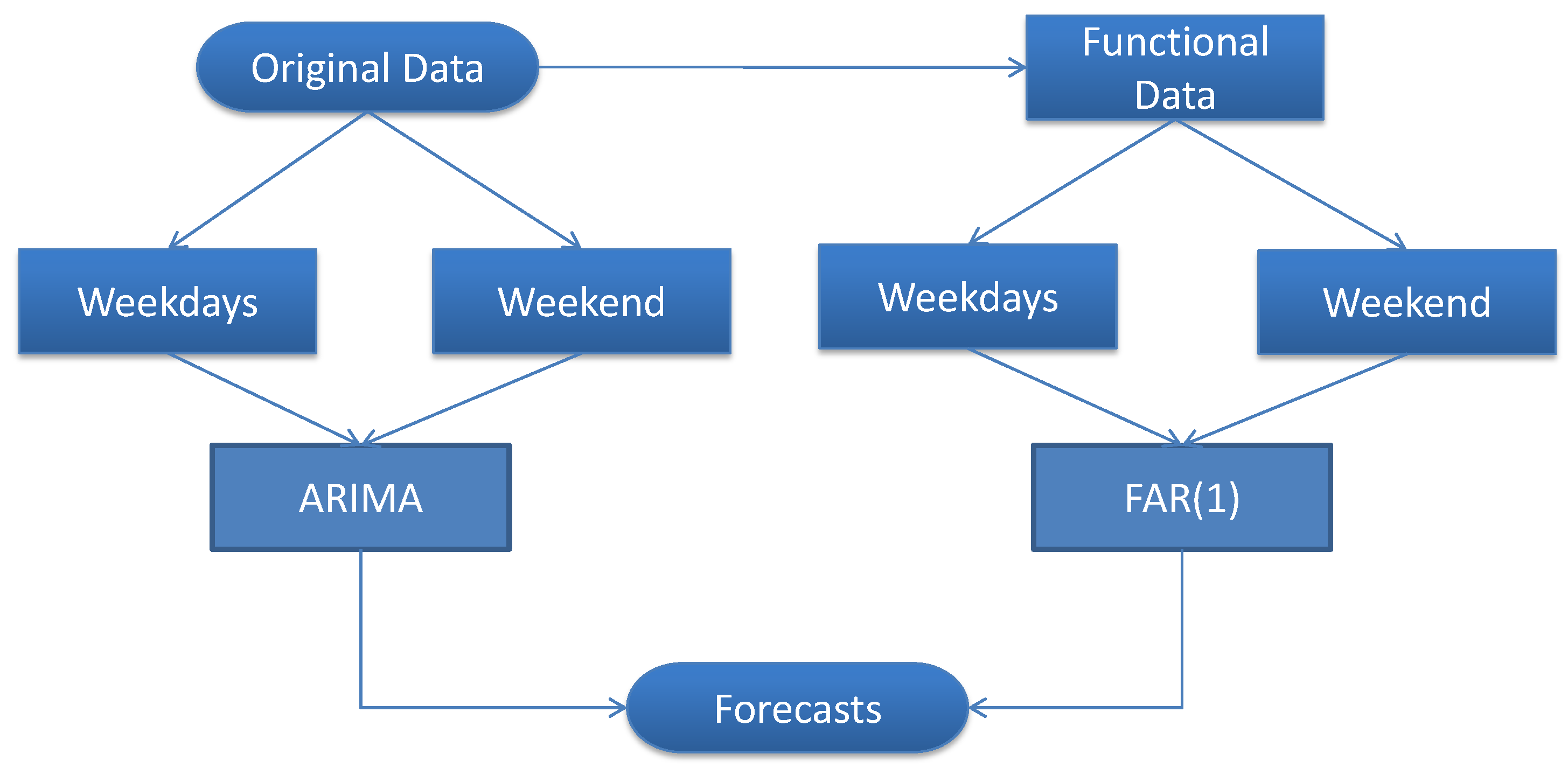
Figure 1. Flowchart of the proposed modeling framework.
Mathematics 10 04279 g001
Figure 2. Daily traffic flow curves for the period 01/01/2016–30/04/2017.
Mathematics 10 04279 g002
Figure 3. Daily traffic flow curves for (top) weekdays (bottom) weekends, for the period 01/01/2016–30/04/2017.
Mathematics 10 04279 g003
Figure 4. Out-of-sample forecasts MAPE values for traffic flow data by (upper panel) FAR(1) and ARIMA(7,1,0) for full data (middle panel) FAR(1) and ARIMA(5,1,0) for weekdays only and (lower panel) FAR(1) and ARIMA(2,1,0) weekends only.
Mathematics 10 04279 g004
Figure 5. Out-of-sample forecasts day specific MAPE (DS-MAPE) values for traffic flow data by (upper panel) FAR(1) and ARIMA(7,1,0) for full data (middle panel) FAR(1) and ARIMA(5,1,0) for weekdays only and (lower panel) FAR(1) and ARIMA(2,1,0) weekends only.
Mathematics 10 04279 g005
Table 1. An example of the traffic flow data set collected at the Dublin airport link road for different days of a week and different time periods of a day.
Date1/1/20162/1/20163/1/20164/1/20165/1/20166/1/20167/1/2016
9:3054411419181510164217331784
11:30986168814371582162415331585
13:301432169719351861177517391654
15:301543183320832002183818961993
17:301323162118622565226425272479
19:30917120913611344136012941474
21:30622621788712777763915
23:30373545473497445399481
Table 2. Accuracy statistics for a one-day ahead out-of-sample traffic flow forecasts.
DaysModelMSEMAEMAPEMSPE
Full dataFAR(1)24,762.96102.019.942.75
ARIMA(7,1,0)38,871.68118.1311.803.90
Working-days onlyFAR(1)21,445.7186.948.242.19
ARIMA(5,1,0)28,791.9799.209.412.58
Weekend days onlyFAR(1)12,228.9680.739.362.170
ARIMA(2,1,0)19,632.8897.4010.302.48
Table 3. Day-specific MAPE from Monday to Sunday.
DaysModelsMAPE for Each Day of the Week
MTWTFSS
Working-days andFAR(1)13.097.667.137.808.6311.4013.66
weekend combineARIMA(7,1,0)14.6511.478.377.0912.1316.3312.54
Working-daysFAR(1)11.517.336.706.209.45
ARIMA(5,1,0)11.879.387.746.8511.21
WeekendFAR(1) 9.279.44
ARIMA(2,1,0) 10.0810.52
Publisher’s Note: MDPI stays neutral with regard to jurisdictional claims in published maps and institutional affiliations.