
Tongue Segmentation and Color Classification Using Deep Convolutional Neural Networks †

Abstract
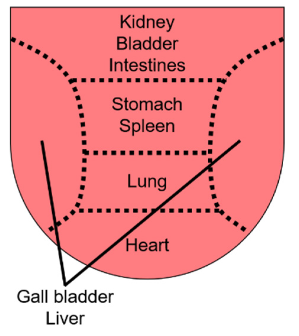
:1. Introduction
2. Related Work
2.1. Tongue Image Segmentation
2.2. Tongue Image Classification
3. Methods
3.1. Atrous Convolution
3.2. Multi-Scale Feature Extraction Methods
3.3. Proposed Methodology
3.3.1. Tongue Segmentation
3.3.2. Tongue Classification
4. Experiment Result and Discussion
4.1. Dataset
4.2. Experiment Result of Segmentation
4.2.1. Evaluation Criterion
4.2.2. Implementation Details
4.2.3. Experimental Results and Analysis
4.3. Experiment Result of Classification
4.3.1. Evaluation Criterion
4.3.2. Implementation Details
4.3.3. Experimental Results and Analysis
- (1)
- Hyper parameter λ
- (2)
- Overall Accuracy
- (3)
- Kappa Coefficient
- (4)
- Individual Sensitivity
- (5)
- The change of loss
- (6)
- Feature visualization
5. Conclusions
Author Contributions
Funding
Data Availability Statement
Conflicts of Interest
References
- Tang, J.; Liu, B.; Ma, K. Traditional Chinese medicine. Lancet 2008, 372, 1938–1940. [Google Scholar] [CrossRef]
- Normile, D. The New Face of Traditional Chinese Medicine. Science 2003, 299, 188–190. [Google Scholar] [CrossRef] [PubMed]
- Zeng, X.; Zhang, Q.; Chen, J.; Zhang, G.; Zhou, A.; Wang, Y. Boundary Guidance Hierarchical Network for Real-Time Tongue Segmentation. arXiv 2020, arXiv:2003.06529. [Google Scholar]
- Zhang, Q.; Shang, H.; Zhu, J.; Jin, M.; Wang, W.; Kong, Q. A new tongue diagnosis application on Android platform. In Proceedings of the 2013 IEEE International Conference on Bioinformatics and Biomedicine, Shanghai, China, 18–21 December 2013. [Google Scholar]
- Pang, B.; Zhang, D.; Li, N.; Wang, K. Computerized tongue diagnosis based on Bayesian networks. IEEE Trans. Biomed. Eng. 2004, 51, 1803–1810. [Google Scholar] [CrossRef] [PubMed] [Green Version]
- Minaee, S.; Boykov, Y.; Porikli, F.; Plaza, A.; Kehtarnavaz, N.; Terzopoulos, D. Image Segmentation Using Deep Learning: A Survey. IEEE Trans. Pattern. Anal. Mach. Intell. 2022, 44, 3523–3542. [Google Scholar] [CrossRef]
- Wei, Y. Tongue Image Segmentation Method Based on Adaptive Thresholds. Comput. Technol. Dev. 2011, 9, 63–65. [Google Scholar]
- Fachrurrozi, M.; Erwin, S. Tongue Image Segmentation using Hybrid Multilevel Otsu Thresholding and Harmony Search Algorithm. J. Phys. Conf. Ser. 2019, 1196, 2072. [Google Scholar] [CrossRef]
- Fu, Z. Tongue Image Segmentation Based on Snake Model and Radial Edge Detection. J. Image. Graph. 2009, 4, 688–693. [Google Scholar]
- Zhang, D.; Zhang, H.; Zhang, B. A Snake-Based Approach to Automated Tongue Image Segmentation. In Tongue Image Analysis; Springer: Hong Kong, China, 2017; pp. 71–88. [Google Scholar]
- Wei, Y.; Fan, P. Application of improved GrabCut method in tongue diagnosis system. Trans. Microsyst. Technol. 2014, 10, 157–160. [Google Scholar]
- Chen, S.; Fu, H. Application of improved graph theory image segmentation algorithm in tongue image segmentation. Comput. Eng. Appl. 2012, 5, 201–203. [Google Scholar]
- Guo, J.; Yang, Y.; Wu, Q. Adaptive active contour model based automatic tongue image segmentation. In Proceedings of the 9th International Congress on Image and Signal Processing, BioMedical Engineering and Informatics (CISP-BMEI 2016), Datong, China, 15–17 October 2016. [Google Scholar]
- Shi, M.; Li, G.; Li, F. C2G2FSnake: Automatic tongue image segmentation utilizing prior knowledge. Sci. China Inf. Sci. 2013, 9, 1–14. [Google Scholar] [CrossRef]
- Li, Q.; Liu, Z. Tongue color analysis and discrimination based on hyperspectral images. Comput. Med. Imaging Graph. 2009, 5, 217–221. [Google Scholar] [CrossRef] [PubMed]
- Cao, G.; Ding, J.; Duan, Y. Classification of tongue images based on doublet and color space dictionary. In Proceedings of the 2016 IEEE International Conference on Bioinformatics and Biomedicine (BIBM), Shenzhen, China, 15–18 December 2016. [Google Scholar]
- Diyana, K.; Yee, O. A Fast SVM-Based Tongue’s Colour Classification Aided by k-Means Clustering Identifiers and Colour Attributes as Computer-Assisted Tool for Tongue Diagnosis. J. Healthc. Eng. 2017, 2017, 7460168. [Google Scholar]
- Ding, J.; Cao, G.; Meng, D. Classification of Tongue Images Based on Doublet SVM. In Proceedings of the International Symposium on System and Software Reliability, Shanghai, China, 29–30 October 2016. [Google Scholar]
- Li, Z.; Pei, Z.; Bo, C. Automatic tongue color analysis of traditional Chinese medicine based on image retrieval. In Proceedings of the International Conference on Control Automation Robotics and Vision, Singapore, 20–22 May 2015. [Google Scholar]
- Niu, G.; Wang, C.; Yan, B.; Pan, Y. Tongue Color Classification Based on Convolutional Neural Network. In Advances in Information and Communication, Proceedings of the 2021 Future of Information and Communication Conference, Vancouver, BC, Canada, 29–30 April 2021; Springer: Cham, Switzerland, 2021. [Google Scholar]
- Wen, Y.; Zhang, K.; Li, Z. A Discriminative Feature Learning Approach for Deep Face Recognition. In Proceedings of the European Conference on Computer Vision, Amsterdam, The Netherlands, 8–16 October 2016. [Google Scholar]
- Guo, A.J.X.; Zhu, F. Spectral-Spatial Feature Extraction and Classification by ANN Supervised With Center Loss in Hyperspectral Imagery. IEEE Trans. Geosci. Remote Sens. 2019, 57, 1755–1767. [Google Scholar] [CrossRef]
- Lu, Y.; Li, X.; Zhang, H.; Zhang, J.; Zhuo, L. Review on Tongue Image Segmentation Technologies for Traditional Chinese Medicine: Methodologies, Performances and Prospects. Acta Autom. Sin. 2021, 47, 1005–1016. [Google Scholar]
- Gao, S.; Guo, N.; Mao, D. LSM-SEC: Tongue Segmentation by the Level Set Model with Symmetry and Edge Constraints. Comput. Intell. Neurosci. 2021, 2021, 6370526. [Google Scholar] [CrossRef] [PubMed]
- Huang, Z.; Miao, J.; Song, H.; Yang, S.; Zhong, Y.; Xu, Q.; Tan, Y.; Wen, C.; Guo, J. A novel tongue segmentation method based on improved U-Net. Neurocomputing 2022, 500, 73–89. [Google Scholar] [CrossRef]
- Qu, P.; Zhang, H.; Zhuo, L. Automatic Tongue Image Segmentation for Traditional Chinese Medicine Using Deep Neural Network. In Proceedings of the Intelligent Computing Theories and Application, Liverpool, UK, 7–10 August 2017. [Google Scholar]
- Lin, B.; Xie, J.; Li, C. Deeptongue: Tongue segmentation via resnet. In Proceedings of the IEEE International Conference on Acoustics, Speech and Signal Processing, Seoul, Republic of Korea, 22–28 April 2018. [Google Scholar]
- Zhou, J.; Zhang, Q.; Zhang, B.; Chen, X. TongueNet: A Precise and Fast Tongue Segmentation System Using U-Net with a Morphological Processing Layer. Appl. Sci. 2019, 9, 3128. [Google Scholar] [CrossRef] [Green Version]
- Mozaffari, M.; Lee, W. Encoder-Decoder CNN Models for Automatic Tracking of Tongue Contours in Real-time Ultrasound Data. Methods 2020, 179, 26–36. [Google Scholar] [CrossRef] [PubMed]
- Hu, Y.; Wen, G.; Liao, H. Automatic construction of Chinese herbal prescription from tongue image via CNNs and auxiliary latent therapy topics. IEEE Trans. Cybern. 2018, 10, 708–721. [Google Scholar]
- Ma, J.; Wen, G.; Hu, Y. Complexity perception classification method for tongue constitution recognition. Artif. Intell. Med. 2019, 96, 123–133. [Google Scholar] [CrossRef] [PubMed]
- Lu, Y.; Li, X.; Gong, Z.; Zhuo, L. TDCCN: A Two-Phase Deep Color Correction Network for Traditional Chinese Medicine Tongue Images. Appl. Sci. 2020, 10, 1784. [Google Scholar] [CrossRef] [Green Version]
- Zhang, J.; Xu, J.; Hu, X.; Chen, Q.; Tu, L.; Huang, J.; Cui, J. Diagnostic Method of Diabetes Based on Support Vector Machine and Tongue Images. Biomed. Res. Int. 2017, 2017, 7961494. [Google Scholar] [CrossRef] [PubMed] [Green Version]
- Mansour, R.F.; Althobaiti, M.M.; Ashour, A.A. Internet of Things and Synergic Deep Learning Based Biomedical Tongue Color Image Analysis for Disease Diagnosis and Classification. IEEE Access 2021, 9, 94769–94779. [Google Scholar] [CrossRef]
- Li, J.; Zhang, Z.; Zhu, X.; Zhao, Y.; Ma, Y.; Zang, J.; Li, B.; Cao, X.; Xue, C. Automatic Classification Framework of Tongue Feature Based on Convolutional Neural Networks. Micromachines 2022, 13, 501. [Google Scholar] [CrossRef]
- Holschneider, M.; Morlet, J. A Real-Time Algorithm for Signal Analysis with the Help of the Wavelet Transform. In Wavelets: Time Frequency Methods and Phase Space; Springer: NewYork, NY, USA, 1989; pp. 286–297. [Google Scholar]
- Krizhevsky, A.; Sutskever, I.; Hinton, G. ImageNet Classification with Deep Convolutional Neural Networks. In Proceedings of the 26th Neural Information Proceeding Systems(NIPS), Nevada City, NV, USA, 3–6 December 2012. [Google Scholar]
- Szegedy, C.; Liu, W.; Jia, Y. Going deeper with convolutions. In Proceedings of the IEEE Conference on Computer Vision and Pattern Recognition, Boston, MA, USA, 7–12 June 2015. [Google Scholar]
- Simonyan, K.; Zisserman, A. Very Deep Convolutional Networks for Large-Scale Image Recognition. In Proceedings of the 3rd International Conference on Learning Representations, San Diego, CA, USA, 7–9 May 2015. [Google Scholar]
- He, K.; Zhang, X.; Ren, S. Deep Residual Learning for Image Recognition. In Proceedings of the IEEE Conference on Computer Vision and Pattern Recognition, Las Vegas, NV, USA, 27–30 June 2016. [Google Scholar]
- Huang, G.; Liu, Z. Densely Connected Convolutional Networks. In Proceedings of the IEEE Conference on Computer Vision and Pattern Recognition, Honolulu, HI, USA, 22–25 July 2017. [Google Scholar]
- He, K.; Zhang, X.; Ren, S. Spatial Pyramid Pooling in Deep Convolutional Networks for Visual Recognition. IEEE Trans. Pattern Anal. Mach. Intell. 2014, 37, 1904–1916. [Google Scholar] [CrossRef] [PubMed] [Green Version]
- Chen, C.; Papandreou, G.; Kokkinos, I. DeepLab: Semantic Image Segmentation with Deep Convolutional Nets, Atrous Convolution, and Fully Connected CRFs. IEEE Trans. Pattern Anal. Mach. Intell. 2018, 40, 838–848. [Google Scholar] [CrossRef] [PubMed] [Green Version]
- Long, J.; Shelhamer, E.; Darrell, T. Fully Convolutional Networks for Semantic Segmentation. IEEE Trans. Pattern Anal. Mach. Intell. 2014, 39, 640–651. [Google Scholar]
- Buda, M.; Maki, A. A systematic study of the class imbalance problem in convolutional neural networks. Neural Netw. 2018, 106, 249–259. [Google Scholar] [CrossRef]
- Ling, C.; Li, C. Data mining for direct marketing: Problems and solutions. In Proceedings of the Fourth International Conference on Knowledge Discovery and Data Mining, New York, NY, USA, 27–31 August 1998. [Google Scholar]
- Kingma, D.; Ba, J. Adam: A Method for Stochastic Optimization. In Proceedings of the 3rd International Conference for Learning Representations, San Diego, CA, USA, 7–9 May 2015. [Google Scholar]
- Cohen, J. Weighted kappa: Nominal scale agreement with provision for scaled disagreement or partial credit. Psychol. Bull. 1968, 70, 213–220. [Google Scholar] [CrossRef]
- Kawaguchi, K.; Kaelbling, L.; Bengio, Y. Generalization in Deep Learning. arXiv 2017, arXiv:1710.05468. [Google Scholar]


| Method | PA | Dice | mIoU |
|---|---|---|---|
| FCN | 89.07% | 88.12% | 87.44% |
| U-net | 93.68% | 93.23% | 92.61% |
| Segnet | 90.95% | 90.15% | 89.54% |
| DeepLabV3+ | 94.53% | 94.02% | 93.27% |
| SegTongue | 97.61% | 97.12% | 96.32% |
| Dataset | Method | SVM Classifier | RF Classifier | Softmax Classifier | Max | |||
|---|---|---|---|---|---|---|---|---|
| OA(%) | Kappa | OA(%) | Kappa | OA(%) | Kappa | |||
| Tongue-2400 | AlexNet | 90.53 | 0.8745 | 90.54 | 0.8739 | 88.25 | 0.8567 | 90.54 |
| A + SSN + CL | 92.38 | 0.9117 | 93.08 | 0.9211 | 92.00 | 0.9067 | 94.08 | |
| DenseNet | 90.79 | 0.8902 | 88.50 | 0.8867 | 88.50 | 0.8867 | 91.79 | |
| D + SSN + CL | 94.17 | 0.9222 | 93.00 | 0.9067 | 92.75 | 0.9033 | 94.17 | |
| Vgg-16 | 90.88 | 0.8917 | 89.04 | 0.8672 | 88.75 | 0.8633 | 91.88 | |
| V + SSN + CL | 96.83 | 0.9578 | 95.67 | 0.9556 | 94.00 | 0.9200 | 96.86 | |
| ResNet-18 | 91.79 | 0.9039 | 88.79 | 0.8772 | 88.25 | 0.8700 | 92.79 | |
| R + SSN + CL | 95.42 | 0.9389 | 93.96 | 0.9328 | 93.25 | 0.9100 | 95.42 | |
| Tongue-2040 | AlexNet | 91.40 | 0.8987 | 91.11 | 0.8948 | 88.11 | 0.8549 | 92.40 |
| A + SSN + CL | 95.05 | 0.9340 | 94.56 | 0.9275 | 92.06 | 0.8941 | 95.05 | |
| DenseNet | 91.47 | 0.8995 | 89.38 | 0.8987 | 88.88 | 0.8784 | 92.07 | |
| D + SSN + CL | 95.87 | 0.9450 | 94.54 | 0.9272 | 93.00 | 0.9067 | 95.87 | |
| Vgg-16 | 91.94 | 0.9059 | 91.11 | 0.8948 | 88.59 | 0.8745 | 92.94 | |
| V + SSN + CL | 97.60 | 0.9680 | 96.50 | 0.9667 | 93.82 | 0.9176 | 97.60 | |
| ResNet-18 | 93.85 | 0.9314 | 91.24 | 0.9098 | 88.29 | 0.8706 | 94.85 | |
| R + SSN + CL | 95.87 | 0.9450 | 94.62 | 0.9417 | 93.25 | 0.9100 | 95.87 | |
| Tongue-1560 | AlexNet | 91.03 | 0.8834 | 91.73 | 0.8897 | 89.62 | 0.8615 | 91.73 |
| A + SSN + CL | 94.35 | 0.9248 | 94.42 | 0.9256 | 94.23 | 0.9231 | 94.42 | |
| DenseNet | 91.51 | 0.9052 | 89.78 | 0.9045 | 89.46 | 0.8861 | 92.91 | |
| D + SSN + CL | 95.77 | 0.9410 | 94.26 | 0.9368 | 93.08 | 0.9077 | 95.77 | |
| Vgg-16 | 91.60 | 0.8880 | 89.47 | 0.8863 | 89.62 | 0.8615 | 91.60 | |
| V + SSN + CL | 97.31 | 0.9641 | 95.05 | 0.9607 | 94.77 | 0.9436 | 97.31 | |
| ResNet-18 | 91.26 | 0.9034 | 89.76 | 0.9034 | 88.38 | 0.8718 | 92.76 | |
| R + SSN + CL | 96.60 | 0.9547 | 94.96 | 0.9462 | 93.85 | 0.9179 | 96.60 | |
| Dataset | Method | SVM Classifier | RF Classifier | Softmax Classifier | |||||||||
|---|---|---|---|---|---|---|---|---|---|---|---|---|---|
| Sens (%) | Sens (%) | Sens (%) | |||||||||||
| 0 | 1 | 2 | 3 | 0 | 1 | 2 | 3 | 0 | 1 | 2 | 3 | ||
| Tongue-2400 | AlexNet | 91.25 | 90.32 | 92.32 | 92.14 | 91.50 | 90.25 | 92.13 | 90.98 | 89.25 | 88.98 | 89.96 | 89.45 |
| A + SSN + CL | 93.38 | 91.23 | 94.23 | 93.98 | 94.08 | 92.30 | 94.25 | 94.09 | 92.67 | 90.58 | 93.25 | 92.36 | |
| DenseNet | 92.17 | 90.28 | 92.15 | 93.09 | 91.50 | 89.59 | 91.23 | 92.45 | 91.50 | 90.56 | 92.54 | 91.35 | |
| D + SSN + CL | 94.17 | 92.15 | 93.48 | 94.89 | 93.00 | 91.25 | 92.56 | 93.96 | 92.69 | 92.03 | 92.98 | 92.21 | |
| Vgg-16 | 91.88 | 91.05 | 92.36 | 92.12 | 90.04 | 88.45 | 89.17 | 90.69 | 89.25 | 88.54 | 89.30 | 89.14 | |
| V + SSN + CL | 96.83 | 95.36 | 96.41 | 96.98 | 96.67 | 95.36 | 96.18 | 96.98 | 93.99 | 92.54 | 94.32 | 94.82 | |
| ResNet-18 | 92.79 | 90.56 | 91.87 | 93.65 | 90.79 | 89.21 | 90.68 | 91.54 | 92.00 | 91.02 | 92.36 | 92.47 | |
| R + SSN + CL | 95.42 | 93.57 | 96.35 | 96.45 | 94.96 | 92.65 | 93.54 | 93.47 | 93.28 | 91.52 | 92.47 | 92.58 | |
| Tongue-2040 | AlexNet | 92.40 | 91.54 | 92.74 | 92.68 | 92.11 | 92.01 | 93.47 | 92.73 | 89.12 | 88.54 | 91.58 | 90.75 |
| A + SSN + CL | 95.05 | 93.47 | 94.12 | 96.36 | 94.56 | 93.57 | 95.18 | 94.85 | 92.08 | 91.58 | 90.54 | 93.58 | |
| DenseNet | 92.47 | 91.05 | 92.85 | 92.83 | 92.08 | 91.58 | 93.47 | 92.36 | 90.88 | 89.25 | 91.58 | 92.84 | |
| D + SSN + CL | 95.88 | 94.35 | 95.98 | 96.02 | 94.54 | 93.69 | 94.58 | 95.12 | 91.67 | 89.21 | 92.50 | 91.58 | |
| Vgg-16 | 92.94 | 91.29 | 92.14 | 93.05 | 92.02 | 91.58 | 93.88 | 94.25 | 90.59 | 90.25 | 91.54 | 90.87 | |
| V + SSN + CL | 97.60 | 95.20 | 96.34 | 97.18 | 97.50 | 96.35 | 98.25 | 97.14 | 93.79 | 90.25 | 94.58 | 94.85 | |
| ResNet-18 | 94.85 | 92.68 | 94.18 | 94.78 | 93.24 | 93.02 | 92.48 | 93.69 | 90.29 | 88.95 | 91.47 | 92.58 | |
| R + SSN + CL | 95.89 | 94.57 | 96.35 | 96.85 | 95.63 | 94.27 | 94.50 | 95.96 | 93.24 | 91.58 | 92.64 | 92.90 | |
| Tongue-1560 | AlexNet | 91.03 | 90.25 | 91.47 | 91.08 | 91.73 | 90.45 | 92.14 | 91.81 | 89.62 | 88.21 | 89.64 | 90.53 |
| A + SSN + CL | 94.36 | 93.56 | 94.20 | 93.05 | 94.42 | 93.12 | 94.82 | 94.62 | 94.63 | 93.58 | 93.47 | 94.18 | |
| DenseNet | 92.93 | 91.05 | 94.84 | 93.67 | 92.78 | 91.58 | 92.69 | 93.14 | 92.46 | 90.51 | 92.82 | 92.64 | |
| D + SSN + CL | 95.58 | 94.05 | 96.77 | 96.14 | 95.26 | 94.25 | 94.58 | 95.84 | 93.56 | 92.84 | 93.64 | 94.76 | |
| Vgg-16 | 91.60 | 92.14 | 91.30 | 91.25 | 91.48 | 90.54 | 91.87 | 92.54 | 89.62 | 88.65 | 91.54 | 92.47 | |
| V + SSN + CL | 97.31 | 95.36 | 97.36 | 96.48 | 97.05 | 96.48 | 98.25 | 98.02 | 95.93 | 93.47 | 94.14 | 94.61 | |
| ResNet-18 | 92.76 | 90.14 | 93.91 | 92.86 | 92.76 | 91.25 | 92.34 | 92.87 | 90.38 | 89.08 | 90.07 | 91.25 | |
| R + SSN + CL | 96.60 | 95.35 | 94.56 | 96.84 | 95.96 | 92.15 | 96.54 | 94.15 | 93.99 | 92.84 | 93.14 | 92.24 | |
Publisher’s Note: MDPI stays neutral with regard to jurisdictional claims in published maps and institutional affiliations. |
© 2022 by the authors. Licensee MDPI, Basel, Switzerland. This article is an open access article distributed under the terms and conditions of the Creative Commons Attribution (CC BY) license (https://creativecommons.org/licenses/by/4.0/).
Share and Cite
Yan, B.; Zhang, S.; Yang, Z.; Su, H.; Zheng, H. Tongue Segmentation and Color Classification Using Deep Convolutional Neural Networks. Mathematics 2022, 10, 4286. https://doi.org/10.3390/math10224286
Yan B, Zhang S, Yang Z, Su H, Zheng H. Tongue Segmentation and Color Classification Using Deep Convolutional Neural Networks. Mathematics. 2022; 10(22):4286. https://doi.org/10.3390/math10224286
Chicago/Turabian StyleYan, Bo, Sheng Zhang, Zijiang Yang, Hongyi Su, and Hong Zheng. 2022. "Tongue Segmentation and Color Classification Using Deep Convolutional Neural Networks" Mathematics 10, no. 22: 4286. https://doi.org/10.3390/math10224286