Testing Multivariate Normality Based on F-Representative Points

Abstract

The multivariate normal is a common assumption in many statistical models and methodologies for high-dimensional data analysis. The exploration of approaches to testing multivariate normality never stops. Due to the characteristics of the multivariate normal distribution, most approaches to testing multivariate normality show more or less advantages in their power performance. These approaches can be classified into two types: multivariate and univariate. Using the multivariate normal characteristic by the Mahalanobis distance, we propose an approach to testing multivariate normality based on representative points of the simple univariate F-distribution and the traditional chi-square statistic. This approach provides a new way of improving the traditional chi-square test for goodness-of-fit. A limited Monte Carlo study shows a considerable power improvement of the representative-point-based chi-square test over the traditional one. An illustration of testing goodness-of-fit for three well-known datasets gives consistent results with those from classical methods.

1. Introduction

The effectiveness of many statistical methodologies relies on the multivariate normal assumption in high-dimensional data analysis. There are various approaches to testing multivariate normality (MVN for short) in the literature (Mardia [1,2,3]; Koziol [4,5]; Mudholkar et al. [6]; Liang and Bentler [7]; Liang et al. [8]; Henze [9]; Mecklin and Mundfrom [10]; Thulin [11]; Szekely and Rizzo [12]; Tenreiro [13]; Kim and Park [14] and Enomoto [15]). As commented in some review papers (Andrews et al. [16]; Gnanadesikan [17]; Looney [18]), it is quite difficult for a single method to beat others completely. To understand the power performance of some frequently-cited methods for testing MVN, Monte Carlo studies have been conducted for comparing these MVN tests (Royston [19,20,21]; Horswell and Looney [22]; Romeu and Ozturk [23]; Young et al. [24]; Beirlant et al. [25]; Mecklin [26]; Mecklin and Mundfrom [27]). In general, when developing a new test, it is compared with a particular category of tests in the literature against a number of alternative distributions, since it would be unreasonable to test every possible deviation from normality (Mecklin and Mundfrom [10]). For example, Ward [28] compared the power of Mardia’s skewness and kurtosis tests, the Malkovich–Afifi test, Hawkins’ test, the Mardia–Foster test, and Ward’s extension of the Kolmogorov–Smirnov and Anderson–Darling tests. It was found none of these tests performed well against the multivariate t-distribution which is a mild deviation from normality. Ahn [29] described a squared jackknife distance and recommended the use of an F-distribution probability plot for checking multivariate normality. Liang et al. [8] constructed projection tests for MVN based on affine invariant statistics. Their tests are still effective in the case of a high dimension with a small sample size. Henze [9] stated that some desirable properties such as affine invariance and consistency are usually required for testing MVN.

There are various approaches to constructing tests for MVN. The idea of statistical representative points or principal points (Fang and He [30]; Flury [31]) is a new approach to constructing goodness-of-fit tests. A set of representative points (RPs for simplicity) refers to selecting a given number of discrete points from a continuous distribution so as to minimize the expected value of the squared distance between the continuous random variable and the set of discrete representative points. In this way, RPs can retain information about the original population as much as possible. The idea of representative points was firstly used in Cox [32] and Max [33] for quantization in univariate normal distribution. Fang [34] applied this concept to the national project of clothing standardization in China and obtained desirable outcomes. Flury [31] applied a similar concept to that in Fang [34] in determining the optimal size of new gas masks and gave the terminology “principal points”. The theoretical foundation, the algorithms for computing RPs, and some associated applications have been developed over the past three decades (Flury [35]; Tarpey [36]; Fang, Zhou, and Wang [37]; Fang, He, and Yang [38]).

In this paper, we propose a new approach to constructing MVN tests, which is based on the RPs of the univariate F-distribution and Pearson’s chi-square test. The new test is based on the squared jackknife distances [29] between each observation and the sample mean, which are affine invariant statistics. As a result, we can avoid estimating unknown parameters $(\mathit{\mu },\mathbf{\Sigma })$ in the d-variate the normal distribution ${\mathrm{N}}_d(\mathit{\mu },\mathbf{\Sigma })$. In Section 2, an MVN test based on RPs of the F-distribution is described. A Monte Carlo study is carried out to investigate the performance of the proposed test in Section 3. Section 4 illustrates the application of the new test to three real examples with computational results from other classical MVN tests. The concluding remarks are summarized in Section 5. All data analysis is performed using the R software (R Development Core Team 2009).

2. The MVN Test Based on the $\mathit{F}$-Representative Points

2.1. A Brief Review on Affine Invariance

A test for MVN is usually expected to have the property of affine invariance. The consequence of this property is that the null distribution of the test statistic does not depend on the unknown mean $\mathit{\mu }$ and covariance matrix $\mathbf{\Sigma }$ of the multivariate normal distribution $N_d(\mathit{\mu },\mathbf{\Sigma })$. Henze ([9], Proposition 2.1) pointed out that any affine invariant test for MVN is a function of the sample Mahalanobis distances (M-distance for short) and angles are defined as follows.

Let $\{{\mathit{x}}_1,\dots ,{\mathit{x}}_n\}$ be a set of i.i.d. (independent identically distributed) sample from a continuous distribution $P^X$. ${\mathcal{N}}_d$ stands for the d-dimensional normal distribution $N_d(\mathit{\mu },\mathbf{\Sigma })$ with mean vector $\mathit{\mu }\in {\mathcal{R}}^d$ and a nonsingular covariance matrix $\mathbf{\Sigma }$. The problem of assessing MVN for the sample is to test the hypothesis

$$H_d:P^X\in {\mathcal{N}}_d$$

(1)

against general alternatives. Any affine invariant statistic $T_n({\mathit{x}}_1,\dots ,{\mathit{x}}_n)$ should satisfy the condition

$$T_n(\mathit{A}{\mathit{x}}_1+\mathit{b},\dots ,\mathit{A}{\mathit{x}}_n+\mathit{b})=T_n({\mathit{x}}_1,\dots ,{\mathit{x}}_n)$$

(2)

for any $\mathit{b}\in {\mathcal{R}}^d$ and nonsingular matrix $\mathit{A}\in {\mathcal{R}}^{d\times d}$. Denote the sample mean and the sample covariance matrix by

$$\overline{\mathit{x}}=\frac{1}{n}\sum _{j=1}^n{\mathit{x}}_i\mathrm{and}{\mathit{S}}_n=\frac{1}{n}\sum _{j=1}^n({\mathit{x}}_j-\overline{\mathit{x}}){({\mathit{x}}_j-\overline{\mathit{x}})}^{\prime },$$

(3)

respectively. The sample M-distance between two observations ${\mathit{x}}_j$ and ${\mathit{x}}_k$ is defined by

$$D_{n,jk}={({\mathit{x}}_j-\overline{\mathit{x}})}^{\prime }{S}_n^{-1}({\mathit{x}}_k-\overline{\mathit{x}}),j,k=1,\dots ,n.$$

(4)

In particular, when $j=k$, denote by

$$D_{n,j}^2=D_{n,jj}={({\mathit{x}}_j-\overline{\mathit{x}})}^{\prime }{\mathit{S}}_n^{-1}({\mathit{x}}_j-\overline{\mathit{x}}).$$

(5)

It is known that any test for MVN based on the M-distance (4) satisfies (2), and so, its null distribution does not depend on the normal parameters $\mu$ and $\mathbf{\Sigma }$. In the following section, we will construct a test for MVN that is a function of the M-distance (4).

2.2. The Jackknife Distance

Define the Jackknife mean and the Jackknife covariance matrix by

$${\overline{\mathit{x}}}_{-i}=\frac{1}{n-1}\sum _{j\ne i}{\mathit{x}}_j\mathrm{and}{\mathit{S}}_{-i}=\frac{1}{n-2}\sum _{j\ne i}({\mathit{x}}_j-{\overline{\mathit{x}}}_{-i}){({\mathit{x}}_j-{\overline{\mathit{x}}}_{-i})}^{\prime },$$

(6)

respectively. The squared Jackknife distance from the i-th observation ${\mathit{x}}_i$ to the sample mean is defined by

$$D_{-i}^2={({\mathit{x}}_i-\overline{\mathit{x}})}^{\prime }{\mathit{S}}_{-i}^{-1}({\mathit{x}}_i-\overline{\mathit{x}}),i=1,\dots ,n.$$

(7)

Ahn [29] employed the squared Jackknife distance (7) to construct an F-probability plot for assessing MVN of the i.i.d. sample $\{{\mathit{x}}_1,\dots ,{\mathit{x}}_n\}$. It is pointed out that the Jackknife covariance matrix ${\mathit{S}}_{-i}$ is related to the usual sample covariance matrix ${\mathit{S}}_n$ in (3) by

$$\frac{1}{n-1}{\mathit{S}}_{-i}^{-1}=\frac{1}{n-1}{\mathit{S}}^{-1}+\frac{{\gamma }_i}{{(n-1)}^2}{\mathit{S}}^{-1}({\mathit{x}}_i-\overline{\mathit{x}}){({\mathit{x}}_i-\overline{\mathit{x}})}^{\prime }{\mathit{S}}^{-1},$$

(8)

where

$$\begin{array}{c}{\displaystyle \mathit{S}=\sum _{j=1}^n({\mathit{x}}_j-\overline{\mathit{x}}){({\mathit{x}}_j-\overline{\mathit{x}})}^{\prime }=n{\mathit{S}}_n,}\\ {\displaystyle {\gamma }_i=\frac{n}{n-1}\left[1-\frac{n}{{(n-1)}^2}\right]{({\mathit{x}}_i-\overline{\mathit{x}})}^{\prime }{\mathit{S}}^{-1}({\mathit{x}}_i-\overline{\mathit{x}}).}\end{array}$$

(9)

The following monotonic relation between the squared Jackknife distance and the usual chi-squared distance is given in [29]:

$$D_{-i}^2=\frac{(n-1)(n-2)D_i^2}{{(n-1)}^2-n{D}_i^2},D_i^2={({\mathit{x}}_i-\overline{\mathit{x}})}^{\prime }{\mathit{S}}^{-1}({\mathit{x}}_i-\overline{\mathit{x}}).$$

(10)

It is obvious that $D_i^2$ is related to the M-distance $D_{n,i}^2$ in (5) by $D_{n,i}^2=n{D}_i^2$. Equations (8)–(10) provide a simple computational method for obtaining the squared Jackknife distances $\{D_{-i}^2:i=1,\dots ,n\}$ by avoiding the computation of n inverse matrices ${\mathit{S}}_{-i}^{-1}$ in (6). The following theorem can be easily derived from [29].

Theorem 1.

Under hypothesis (1), the following two assertions are true:

(1) 

the adjusted Jackknife distance has an exact F-distribution:

$$d_{-i}^2=\frac{n(n-1-d)}{(n-1)(n-2)d}{D}_{-i}^2\sim F(d,n-1-d);$$

(11)

(2) 

$\{d_{-i}^2:i=1,\dots ,n\}$ are asymptotically independent.

Proof of Theorem 1.

The exact F-distribution for each $d_{-i}$ in (11) is given in Theorem 1 of Ahn [29]. The asymptotic independence of $\{d_{-i}^2:i=1,\dots ,n\}$ can be verified as follows. According to the strong law of convergence,

$$\overline{\mathit{x}}\stackrel{\mathrm{a}.\mathrm{s}}{\to }\mathit{\mu },(n\to \infty )$$

where $\stackrel{\mathrm{a}.\mathrm{s}}{\to }$ means “converge almost surely”. ${\mathit{S}}_n$ can be written as

$${\mathit{S}}_n=\frac{1}{n}\sum _{i=1}^n({\mathit{x}}_i-\mathit{\mu }){({\mathit{x}}_i-\mathit{\mu })}^{\prime }+(\overline{\mathit{x}}-\mathit{\mu }){(\overline{\mathit{x}}-\mathit{\mu })}^{\prime }.$$

Because

$$\frac{1}{n}\sum _{i=1}^n({\mathit{x}}_i-\mathit{\mu }){({\mathit{x}}_i-\mathit{\mu })}^{\prime }$$

is the sample mean of the i.i.d. terms $({\mathit{x}}_i-\mathit{\mu }){({\mathit{x}}_i-\mathit{\mu })}^{\prime }$, the strong law of convergence (page 238, Theorem 1 of Feller, [39]) gives

$$\frac{1}{n}\sum _{i=1}^n({\mathit{x}}_i-\mathit{\mu }){({\mathit{x}}_i-\mathit{\mu })}^{\prime }\stackrel{\mathrm{a}.\mathrm{s}}{\to }E\left\{({\mathit{x}}_i-\mathit{\mu }){({\mathit{x}}_i-\mathit{\mu })}^{\prime }\right\}=\mathbf{\Sigma }.$$

According to the continuous mapping theorem (page 7, Van der Vaart [40]), it follows that

$$(\overline{\mathit{x}}-\mathit{\mu }){(\overline{\mathit{x}}-\mathit{\mu })}^{\prime }\stackrel{\mathrm{a}.\mathrm{s}}{\to }\mathbf{0},S_n=\frac{1}{n}\sum _{i=1}^n({\mathit{x}}_i-\mathit{\mu }){({\mathit{x}}_i-\mathit{\mu })}^{\prime }+(\overline{\mathit{x}}-\mathit{\mu }){(\overline{\mathit{x}}-\mathit{\mu })}^{\prime }\stackrel{\mathrm{a}.\mathrm{s}}{\to }\mathbf{\Sigma },(n\to \infty )$$

and

$$n{D}_i^2\stackrel{\mathrm{a}.\mathrm{s}}{\to }{({\mathit{x}}_i-\mathit{\mu })}^{\prime }{\mathbf{\Sigma }}^{-1}({\mathit{x}}_i-\mathit{\mu }),n{D}_j^2\stackrel{\mathrm{a}.\mathrm{s}}{\to }{({\mathit{x}}_j-\mathit{\mu })}^{\prime }{\mathbf{\Sigma }}^{-1}({\mathit{x}}_j-\mathit{\mu })(n\to \infty )$$

for any given $i\ne j$. The independence between ${\mathit{x}}_i$ and ${\mathit{x}}_j$ results in the asymptotic independence between $n{D}_i^2$ and $n{D}_j^2$ for $i\ne j$. Because $d_{-i}^2$ is a continuous function of $n{D}_i^2$ for $i=1,\dots ,n$, using the continuous mapping theorem again, we can obtain the asymptotic independence of $\{d_{-i}^2:i=1,\dots ,n\}$ in (11). This completes the proof.    □

2.3. The Chi-Squared Test Based on the F-Representative Points

The above Theorem 1 provides an approach to testing hypothesis (1). Instead of testing (1), we can test

$$H_0:\{d_{-i}^2:i=1,\dots ,n\}\mathrm{in}\left(11\right)\mathrm{is}\mathrm{sample}\mathrm{from}F(d,n-1-d)$$

(12)

against the alternative that $H_0$ is not true. It is obvious that if hypothesis (12) is rejected, hypothesis (1) is also rejected, but the converse is not true. A test for hypothesis (12) is called a necessary test [41] for the normality of the original data in the literature. Testing hypothesis (12) can be carried out by the classical chi-squared test for the purpose of general goodness of fit. It is well-known that the classical chi-squared test is facing the choice of classification cells for observed sample data (Sturges [42]; Mann and Wald [43]; Williams [44]; Dahiya and Gurland [45]; Mineo [46]; Harrison [47]; Kallenberg [48,49]; Oosterhoff [50]; Quine and Robinson [51]; D’Agostini and Stephens [52]; Koehler and Gann [53]; Bogdan [54]). A classification with equiprobable cells is a common choice in the literature. Because the representative points minimize some kind of quadratic loss function (see Appendix A), we conjecture that classification cells based on representative points may have better performance than the simple equiprobable classification. Therefore, we propose to use the F-representative points to construct classification cells and expect to improve the performance of the classical chi-squared test. A Monte study will be carried out in next section to verify the performance of this approach.

The F-representative points are a set of points $\{F_1,\dots ,F_m\}$ (for a selected number of points m) that minimize the quadratic loss function:

$$\varphi (x_1,\dots ,x_m)={\int }_0^{\infty }\underset{1\le i\le m}{min}\left\{{(x_i-x)}^2\right\}{f}_F(x;d,n-1-d)dx,$$

(13)

where $f_F(x;d,n-1-d)$ stands for the density function of the F-distribution with degrees of freedom $(d,n-1-d)$,

$$\varphi (F_1,\dots ,F_m)=\underset{1\le i\le m}{min}\{\varphi (x_1,\dots ,x_m):0<x_1<\dots <x_m<\infty \}.$$

Define the following intervals

$$\begin{array}{c}{\displaystyle I_1=\left(0,\frac{F_1+F_2}{2}\right),I_2=\left[\frac{F_1+F_2}{2},\frac{F_2+F_3}{2}\right),\dots ,}\\ {\displaystyle I_{m-1}=\left[\frac{F_{m-2}+F_{m-1}}{2},\frac{F_{m-1}+F_m}{2}\right),I_m=\left[\frac{F_{m-1}+F_m}{2},+\infty \right)}\end{array}$$

(14)

and the probabilities

$$p_i={\int }_{I_i}{f}_F(x;d,n-1-d)dx,i=1,\dots ,m.$$

(15)

According to Fang and He [30], $\{p_1,\dots ,p_m\}$ can be considered as a set of “representative probabilities” for the F-distribution $F(d,n-1-d)$.

Based on Theorem 1 above, a test for hypothesis (1) can be approximately (under large sample size n) transferred to testing (12) with classification intervals defined by (14). The ${\chi }^2$-statistic is computed by:

$${\chi }_R^2=\sum _{i=1}^m\frac{{(n_i-n{p}_i)}^2}{n{p}_i}\to {\chi }^2(m-1),(n\to \infty \mathrm{under}\mathrm{the}\mathrm{hypothesis}\left(1\right))$$

(16)

where $n_i$ is the frequency of the transformed approximately i.i.d. sample points $\{d_{-i}^2:i=1,\dots ,n\}$ computed by (11) that are located in the interval $I_i$ in (14). The approximate p-value is computed by

$$P({\chi }_R^2,\nu )=K{\int }_{{\chi }_R^2}^{\infty }{z}^{\frac{\nu }{2}-1}exp(-\frac{z}{2})dz,\mathrm{with}\nu =m-1,K={\left[2^{\frac{\nu }{2}}\mathrm{\Gamma }\left(\frac{\nu }{2}\right)\right]}^{-1}.$$

(17)

The Monte Carlo study in the next section will verify how well the chi-square approximation (16) is by simulating the empirical type I error rates and its power against some selected sets of alternative distributions.

3. A Monte Carlo Study

In order to compare the ${\chi }^2$-test (16) under the “representative probabilities” $\{p_1,\dots ,p_m\}$ in (15) with the traditional chi-squared test, we choose the equiprobable cells for computing the traditional chi-squared test. For a selected number of points $m-1$, define the interval endpoints:

$$\begin{array}{c}{\displaystyle a_1\mathrm{satisfies}P({\chi }^2(m-1)<a_1)=\frac{1}{m};}\hfill \\ {\displaystyle a_2\mathrm{satisfies}P(a_1<{\chi }^2(m-1)<a_2)=\frac{1}{m};}\hfill \\ ⋮\hfill \\ {\displaystyle a_{m-1}\mathrm{satisfies}P({\chi }^2(m-1)>a_{m-1})=\frac{1}{m}.}\hfill \end{array}$$

(18)

Denote the traditional chi-squared test based on the interval endpoints (18) by ${\chi }_T^2$ which also has an approximate null distribution χ²(m − 1),

$${\chi }_T^2=\sum _{i=1}^m\frac{{(N_i-n/m)}^2}{n/m}$$

(19)

where $N_i$ is the frequency of the approximate i.i.d. transformed sample points $\{d_{-i}^2:i=1,\dots ,n\}$ that are located in the i-th interval.

3.1. A Comparison between Empirical Type I Error Rates

Because the chi-squared test based on the transformed sample points $\{d_{-i}^2:i=1,\dots ,n\}$ given by (11) are affine invariant under any nonsingular linear transformation of the original i.i.d. sample $\{{\mathit{x}}_1,\dots ,{\mathit{x}}_n\}$, we only need to generate samples from a d-dimensional standard normal $N_d(\mathbf{0},{\mathit{I}}_d)$ (${\mathit{I}}_d$ stands for the $d\times d$ identity matrix). The simulation results under 2000 replications for each case are summarized in

Table 1. Empirical type I error rates ($\alpha =0.05$).

n	m	Test	$\mathit{d}=3$	$\mathit{d}=5$	$\mathit{d}=10$	$\mathit{d}=15$	$\mathit{d}=20$
$n=20$	$m=10$	${\chi }_R^2$	0.056	0.060	0.064	0.056	0.072
		${\chi }_T^2$	0.040	0.022	0.032	0.030	0.024
	$m=20$	${\chi }_R^2$	0.050	0.070	0.061	0.064	0.062
		${\chi }_T^2$	0.038	0.026	0.038	0.038	0.022
	$m=30$	${\chi }_R^2$	0.062	0.070	0.064	0.074	0.078
		${\chi }_T^2$	0.042	0.032	0.036	0.038	0.028
$n=50$	$m=10$	${\chi }_R^2$	0.032	0.035	0.048	0.046	0.035
		${\chi }_T^2$	0.027	0.030	0.039	0.038	0.033
	$m=20$	${\chi }_R^2$	0.049	0.059	0.059	0.065	0.064
		${\chi }_T^2$	0.037	0.036	0.034	0.036	0.035
	$m=30$	${\chi }_R^2$	0.057	0.074	0.072	0.070	0.082
		${\chi }_T^2$	0.038	0.037	0.033	0.037	0.040
$n=100$	$m=10$	${\chi }_R^2$	0.032	0.034	0.048	0.046	0.035
		${\chi }_T^2$	0.025	0.031	0.034	0.025	0.036
	$m=20$	${\chi }_R^2$	0.062	0.067	0.044	0.048	0.054
		${\chi }_T^2$	0.041	0.025	0.038	0.032	0.031
	$m=30$	${\chi }_R^2$	0.059	0.060	0.065	0.060	0.062
		${\chi }_T^2$	0.040	0.036	0.043	0.036	0.032
$n=200$	$m=10$	${\chi }_R^2$	0.041	0.038	0.022	0.028	0.030
		${\chi }_T^2$	0.034	0.038	0.025	0.030	0.031
	$m=20$	${\chi }_R^2$	0.057	0.046	0.041	0.043	0.041
		${\chi }_T^2$	0.036	0.038	0.032	0.040	0.040
	$m=30$	${\chi }_R^2$	0.072	0.069	0.051	0.039	0.049
		${\chi }_T^2$	0.042	0.046	0.039	0.034	0.039
$n=400$	$m=10$	${\chi }_R^2$	0.027	0.034	0.034	0.038	0.037
		${\chi }_T^2$	0.036	0.032	0.032	0.037	0.036
	$m=20$	${\chi }_R^2$	0.043	0.041	0.037	0.045	0.047
		${\chi }_T^2$	0.040	0.033	0.039	0.032	0.033
	$m=30$	${\chi }_R^2$	0.058	0.054	0.046	0.050	0.044
		${\chi }_T^2$	0.042	0.033	0.041	0.036	0.037
$n=1000$	$m=10$	${\chi }_R^2$	0.034	0.038	0.036	0.050	0.042
		${\chi }_T^2$	0.032	0.038	0.028	0.036	0.044
	$m=20$	${\chi }_R^2$	0.038	0.044	0.042	0.042	0.040
		${\chi }_T^2$	0.044	0.054	0.050	0.060	0.028
	$m=30$	${\chi }_R^2$	0.034	0.046	0.036	0.054	0.042
		${\chi }_T^2$	0.032	0.046	0.026	0.046	0.038

. It shows that both statistics ${\chi }_R^2$ and ${\chi }_T^2$ control their empirical type I error rates reasonably well under the significant level 0.05. For most of cases, ${\chi }_T^2$ is more conservative than ${\chi }_R^2$, especially for a smaller sample size. They have similar performance for significant levels 0.01 and 0.10 for which the simulation outcomes are not presented here to save space.

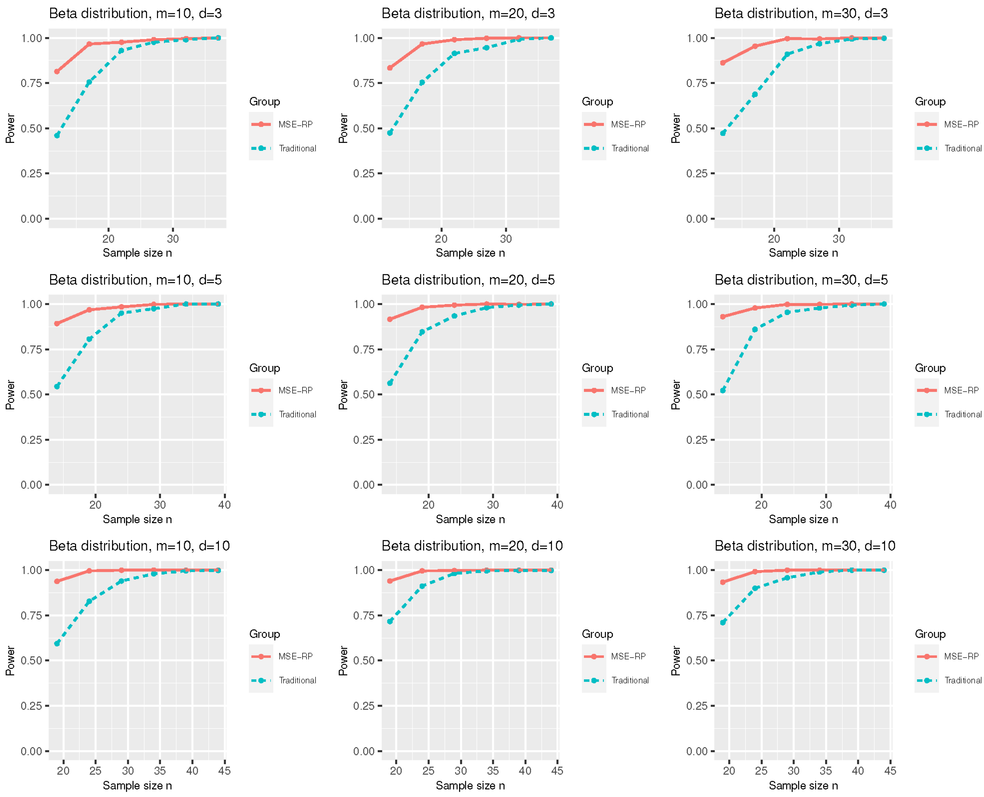
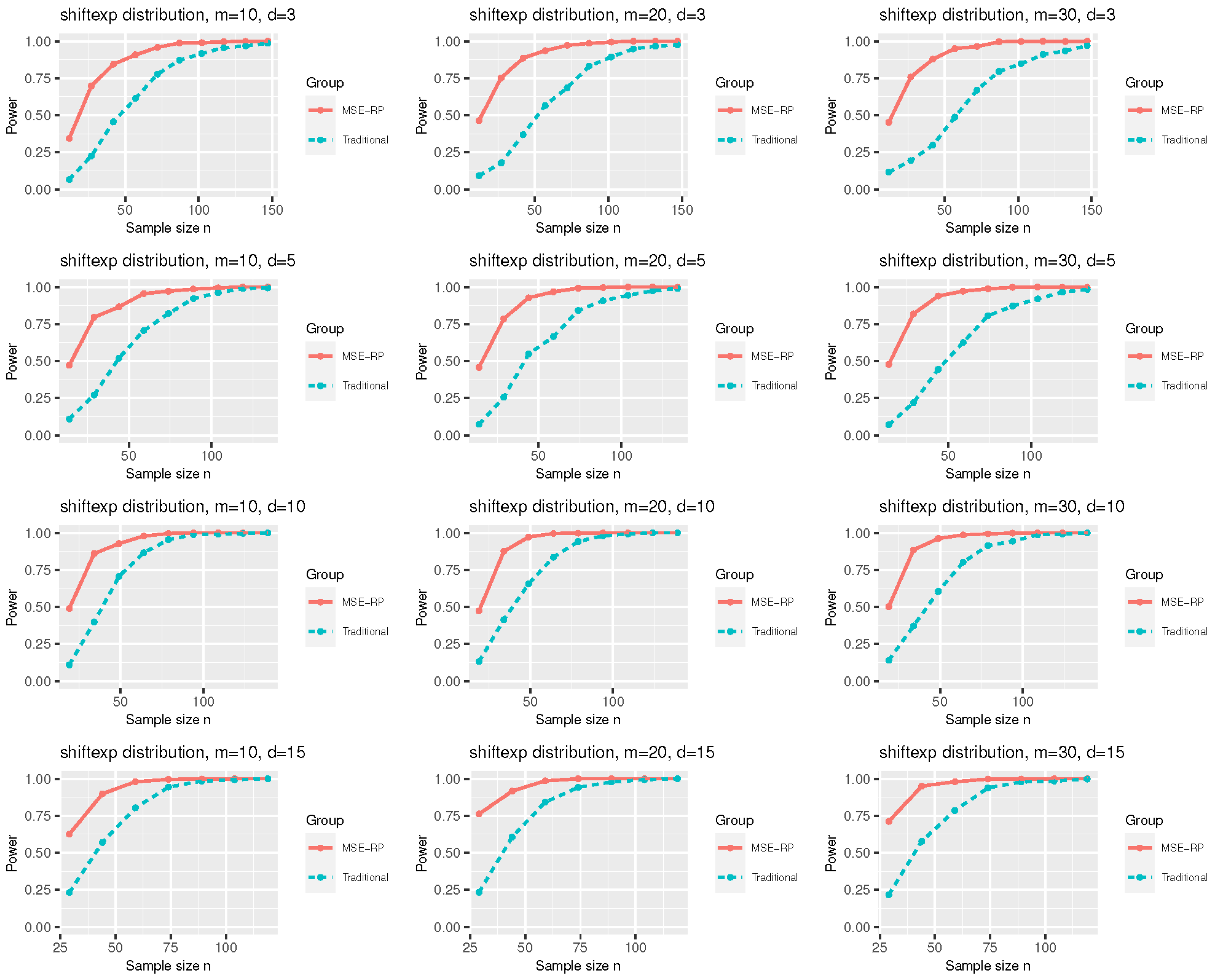
3.2. A Power Comparison

The following alternative distributions are selected.

(1)

The multivariate t-distribution has a density function of the form

$$f_t(\parallel \mathit{x}\parallel )=C_1{\left(1+\frac{{\parallel \mathit{x}\parallel }^2}{v}\right)}^{-\frac{d+v}{2}},v>0,$$

where “$\parallel ·\parallel$” stands for the Euclidean norm of a vector, and let the degree of freedom $v=5$;

(2)

The $\beta$-generalized normal distribution $N_d(\mathbf{0},{\mathit{I}}_d,1/2)$ with $\beta =1/2$ has a density function of the form by (Goodman and Kotz [55]):

$$f(x_1,\dots ,x_d)=\frac{{\beta }^d{r}^{d/\beta }}{2^d{\mathrm{\Gamma }}^d(1/\beta )}·exp\left\{-r\sum _{i=1}^d{\left|x_i\right|}^{\beta }\right\},{(x_1,\dots ,x_d)}^{\prime }\in R^d,$$

where $r>0$ is a parameter. Let $r=1/2$ in the simulation and denote it by $\beta$ g-normal;

(3)

The shifted i.i.d. ${\chi }^2\left(1\right)$ with i.i.d. marginals, each marginal has the same distribution as that of the random variable $Y=X-E\left(X\right)$, where $X\sim {\chi }^2\left(1\right)$, the univariate chi-squared distribution with 1 degree of freedom and $E\left(X\right)=1$;

(4)

The distribution $N(0,1)+{\chi }^2\left(2\right)$ consists of i.i.d. $[d/2]$ normal $N(0,1)$ marginals and $d-[d/2]$ i.i.d. ${\chi }^2\left(2\right)$ marginals, where $[d/2]$ stands for the integer part of $d/2$;

(5)

The shifted i.i.d. $exp\left(1\right)$ with i.i.d. marginals, each marginal has the same distribution as that of the random variable $Y=X-E\left(X\right)$, where $X\sim exp\left(1\right)$, the univariate exponential distribution.

For each of these alternative distributions, we choose the sample size $n=20,\dots ,400$. By simulation with 10,000 replications, the power values versus the sample size n for both statistics ${\chi }_R^2$ in (18) and ${\chi }_T^2$ computed via (19) are plotted in Figure 1, Figure 2, Figure 3, Figure 4 and Figure 5. As can be seen, the proposed statistic ${\chi }_R^2$ obviously outperforms the classical ${\chi }_T^2$ for different alternative distributions consistently. It shows a clear trend that the chi-squared statistic ${\chi }_R^2$ based on F-representative points can be quite successful in improving the performance of traditional chi-squared statistic ${\chi }_T^2$. To see the power performance of ${\chi }_R^2$ versus other frequently used tests in the literature, we choose a category of tailor-made MVN tests in the literature (Mardia [3]; Henze and Wagner [56]; Szekely and Rizzo [57]) against two types of alternative distributions (symmetric and non-symmetric) in Figure 6 and Figure 7 where “hz” stands for Henze and Wagner’s statistic and “energy” for Szekely and Rizzo’ test. The simple comparison in Figure 6 and Figure 7 shows that the ${\chi }_R^2$-test based on F-representative points can be comparable to the selected frequently used tests in the literature. More power comparisons based on three additional alternative distributions are given in Appendix C. This gives some confidence in using the ${\chi }_R^2$-test as a supplement to enhance the application of some existing tests.

4. Illustrative Examples

Example 1—Ramus Bone Data. Elston and Grizzle [58] collected interesting data on the ramus height (in millimeters) of 20 boys each measured at age 8, 8.5, 9, and 9.5 years old. The objective of the original study is to establish a normal growth curve for use by orthodontists. The data has a few interesting features. Timm [59] showed that the recorded heights of the ramus bone marginally appear to be normally distributed but show a certain departure from multivariate normality for $\alpha =0.05$. To test the multivariate normality of ages 8, 8.5, 9, and 9.5, the methods proposed by Zhou and Shao [60] gave p-values 0.002, 0.054, <0.001, <0.001.

Example 2—Fisher’s Iris Data. Fisher’s Iris dataset examined by R.A. Fisher demonstrated the initial study of discriminant analysis in 1936 [61]. In this well-known example of multivariate data, three varieties of iris flowers are measured (setosa, versicolor and virginica), consisting of a total of 150 observations (50 each) in terms of four measurements: sepal length, sepal width, petal length, petal width. Considering the multivariate normality of the four measurements, Srivastava and Mudholkar [62] concluded that the assumption of multivariate normality may not be appropriate in the context of any of the varieties of Iris. Furthermore, Shao and Zhou [63] rejected multivariate normality for this dataset using different tests with all p-values $<2\%$ at level $\alpha =5\%$ which is also consistent with the findings in Small [64].

Example 3—Rao’s Cork Data. The dataset collected by Rao [65] measured the weight of cork borings taken from the north (N), east (E), south (S), and west (W) directions which consisted of the thickness of bark deposit in 28 corks. The original problem is to investigate whether the bark deposit varies in thickness in the four directions. Regarding the multivariate normality assumption, Srivastava and Hui [66] rejected the hypothesis using tests with p-values of 0.01 and 0.037. Moreover, Mudholkar, McDermott, and Srivastava [6] also doubted the multivariate normality assumption based on their p-value of $0.0302$. Srivastava and Mudholkar [62] applied the simplified Fisher combination statistic and obtained a p-value of $0.006$, which also implies certain departure from multivariate normality.

To assess the assumption of multivariate normality for these data by the two chi-squared tests ${\chi }_R^2$ and ${\chi }_T^2$, the p-values under different m (the number of representative points) from the two chi-squared tests ${\chi }_R^2$ in (16) and ${\chi }_T^2$ computed via (19) are summarized in following

Table 2. p-values from the two chi-squared tests.

Variables	${\mathit{\chi }}^2$-Test	$\mathit{m}=10$	$\mathit{m}=20$	$\mathit{m}=30$
$\left(X_8,X_{8.5},X_9,X_{9.5}\right)$	${\chi }_R^2$	0.0016	$1.661\times {10}^{-6}$	0.0005
	${\chi }_T^2$	0.0669	0.1302	0.0839
$\left(X_{sl},X_{sw},X_{pl},X_{pw}\right)$	${\chi }_R^2$	0.0066	0.0199	0.0076
	${\chi }_T^2$	0.0179	0.0397	0.0979
$\left(X_N,X_E,X_S,X_W\right)$	${\chi }_R^2$	0.0004	<10${}^{-10}$	<10${}^{-10}$
	${\chi }_T^2$	0.7110	0.3610	0.7566

. Meanwhile, we use the classical skewness, kurtosis and univariate Shapiro–Wilk tests [67] to assess the marginal normality of each of the four variables.

Table 3. Skewness and Kurtosis for each measurement and feature.

Variables	Skewness	Kurtosis	UVN Test 1	Mardia’s MVN Test 2
$X_8$	0.3069	−1.0682	0.3360	Sk: 0.0093
$X_{8.5}$	0.3111	−0.8932	0.6020	Ku: 0.1125
$X_9$	0.0645	−1.2076	0.5016
$X_{9.5}$	0.0648	−1.4332	0.0905
$X_{sl}$	0.3118	−0.5736	0.0102	Sk: $4.7570\times {10}^{-7}$
$X_{sw}$	0.3158	0.1810	0.1012	Ku: 0.8180
$X_{pl}$	−0.2721	−1.3955	<0.0001
$X_{pw}$	−0.1019	−1.3361	<0.0001
$X_N$	0.8088	−0.3535	0.0179	Sk: $7.6249\times {10}^{-9}$
$X_E$	0.8322	−0.2680	0.0135	Ku: 0.0076
$X_S$	−0.1289	−0.3767	0.0361
$X_W$	0.4417	−0.7800	0.1185

¹p-values from univariate Shapiro-Wilk tests. ²p-values from Mardia’s multivariate skewness and kurtosis tests.

also gives the results of the p-values of the two statistics for skew and kurtosis from Mardia’s MVN test. The variables in the following two tables are:

$$\begin{array}{ccc}{X}_8\hfill & =\hfill & {\mathrm{boys}}^{\prime } \mathrm{ramus} \mathrm{height} \mathrm{at} \mathrm{age} 8 \mathrm{in} \mathrm{Example} 1\hfill \\ X_{8.5}\hfill & =\hfill & {\mathrm{boys}}^{\prime } \mathrm{ramus} \mathrm{height} \mathrm{at} \mathrm{age} 8.5 \mathrm{in} \mathrm{Example} 1\hfill \\ X_9\hfill & =\hfill & {\mathrm{boys}}^{\prime } \mathrm{ramus} \mathrm{height} \mathrm{at} \mathrm{age} 9 \mathrm{in} \mathrm{Example} 1\hfill \\ X_{9.5}\hfill & =\hfill & {\mathrm{boys}}^{\prime } \mathrm{ramus} \mathrm{height} \mathrm{at} \mathrm{age} 9.5 \mathrm{in} \mathrm{Example} 1\hfill \\ X_{sl}\hfill & =\hfill & \mathrm{sepal} \mathrm{length} \mathrm{in} \mathrm{Example} 2\hfill \\ X_{sw}\hfill & =\hfill & \mathrm{sepal} \mathrm{width} \mathrm{in} \mathrm{Example} 2\hfill \\ X_{pl}\hfill & =\hfill & \mathrm{petal} \mathrm{length} \mathrm{in} \mathrm{Example} 2\hfill \\ X_{pw}\hfill & =\hfill & \mathrm{petal} \mathrm{width} \mathrm{in} \mathrm{Example} 2\hfill \\ X_N\hfill & =\hfill & \mathrm{the} \mathrm{weight} \mathrm{of} \mathrm{cork} \mathrm{borings} \mathrm{taken} \mathrm{from} \mathrm{north} \mathrm{in} \mathrm{Example} 3\hfill \\ X_E\hfill & =\hfill & \mathrm{the} \mathrm{weight} \mathrm{of} \mathrm{cork} \mathrm{borings} \mathrm{taken} \mathrm{from} \mathrm{east} \mathrm{in} \mathrm{Example} 3\hfill \\ X_S\hfill & =\hfill & \mathrm{the} \mathrm{weight} \mathrm{of} \mathrm{cork} \mathrm{borings} \mathrm{taken} \mathrm{from} \mathrm{south} \mathrm{in} \mathrm{Example} 3\hfill \\ X_W\hfill & =\hfill & \mathrm{the} \mathrm{weight} \mathrm{of} \mathrm{cork} \mathrm{borings} \mathrm{taken} \mathrm{from} \mathrm{west} \mathrm{in} \mathrm{Example} 3\hfill \end{array}$$

The p-values from the representative-points chi-squared test ${\chi }_R^2$ in Table 2 clearly indicate the significant departure from joint multivariate normality for the four variables in each example, while the p-values from the traditional chi-squared test ${\chi }_T^2$ only partially imply a certain departure from joint multivariate normality. The potential departure from joint multivariate normality is also convinced by Mardia’s multivariate skewness test and most of the univariate normality tests (UVN tests in Table 3) by Shapiro–Wilk’s statistic. Because the results from ${\chi }_R^2$-test are nearly all consistent with those from the well-performed tests in the literature, the representative-point-based ${\chi }_R^2$-test seems to give more consistent results with some well-known existing tests than does the traditional ${\chi }_T^2$-test.

5. Concluding Remarks

Testing multivariate normality is a long-lasting research direction in the area of testing goodness-of-fit. There have been various approaches to constructing the goodness-of-fit tests in the literature. The representative-points approach in this paper provides a different angle to modify the classical Pearson–Fisher chi-squared test for multivariate probability distributions such as the multivariate normal. The limited Monte Carlo study in the paper demonstrates the remarkable power improvement of the representative-points chi-squared test over the traditional equiprobable chi-squared test. Although it is difficult to theoretically prove why the representative-points chi-squared test can improve the traditional equiprobable chi-squared test, we discover an implementable way to extend the application of the theory of statistical representative points. More importantly, the simple power comparison with other multivariate normality tests in Figure 6 and Figure 7 implies that the representative-points-based chi-squared test can have competitive power performance with some well-known existing tests in the literature. It should be pointed out that the representative-points-based chi-square test in this paper is only a “necessary test” [68] for multivariate normality, which means that if the null hypothesis is rejected by ${\chi }_R^2$ in (16), one can definitely conclude the departure from multivariate normality. However, if the test fails to reject the null hypothesis, there is no guarantee to ensure multivariate normality. This implies that the test in this paper possesses the same weakness as do many existing tests for multivariate normality. The representative-points approach to constructing goodness-of-fit sheds some additional light on the rich literature in testing multivariate normality. This paper provides some ideas to improve some other existing tests (e.g., Malkovich [69]; McAssey [70]) for multivariate normality by using Jackknife distance and statistical representative points.

References

1. Mardia, K.V. Measures of multivariate skewnees and kurtosis with applications. Biometrika 1970, 57, 519–530. [Google Scholar] [CrossRef]
2. Mardia, K.V. Applications of some measures of multivariate skewness and kurtosis for testing normality and robustness studies. Sankhy A 1974, 36, 115–128. [Google Scholar]
3. Mardia, K.V. Tests of univariate and multivariate normality. Handb. Stat. 1980, 1, 297–320. [Google Scholar]
4. Koziol, J.A. A class of invariant procedures for assessing multivariate normality. Biometrika 1982, 69, 423–427. [Google Scholar] [CrossRef]
5. Koziol, J.A. Assessing multivariate normality: A compendium. Commun. Stat. Theory Methods 1986, 15, 2763–2783. [Google Scholar] [CrossRef]
6. Mudholkar, G.S.; McDermott, M.; Srivastava, D.K. A test of p-variate normality. Biometrika 1992, 79, 850–854. [Google Scholar] [CrossRef]
7. Liang, J.; Bentler, P.M. A t-distribution plot to detect non-multinormality. Comput. Stat. Data Anal. 1995, 30, 31–44. [Google Scholar] [CrossRef]
8. Liang, J.; Li, R.; Fang, H.; Fang, K.T. Testing multinormality based on low-dimensional projection. J. Stat. Plan. Inference 2000, 86, 129–141. [Google Scholar] [CrossRef]
9. Henze, N. Invariant tests for multivariate normality: A critical review. Stat. Papers 2002, 43, 467–507. [Google Scholar] [CrossRef]
10. Mecklin, C.J.; Mundfrom, D.J. An appraisal and bibliography of tests for multivariate normality. Int. Stat. Rev. 2004, 72, 123–138. [Google Scholar] [CrossRef]
11. Thulin, M. Tests for multivariate normality based on canonical correlations. Stat. Meth. Appl. 2014, 23, 189–208. [Google Scholar] [CrossRef] [Green Version]
12. Szekely, G.J.; Rizzo, M.L. Energy statistics: A class of statistics based on distances. J. Stat. Plan. Inference 2013, 143, 1249–1272. [Google Scholar] [CrossRef]
13. Tenreiro, C. A new test for multivariate normality by combining extreme and nonextreme BHEP tests. Commun. Stat. Simul. Comput. 2017, 46, 1746–1759. [Google Scholar] [CrossRef]
14. Kim, I.; Park, S. Likelihood ratio test for multivariate normality. Commun. Stat. Theory Meth. 2018, 47, 1923–1934. [Google Scholar] [CrossRef]
15. Enomoto, R.; Hanusz, Z.; Hara, A.; Seo, T. Multivariate normality test using normalizing transformation for Mardia’s multivariate kurtosis. Commun. Stat. Simul. Comput. 2020, 49, 684–698. [Google Scholar] [CrossRef]
16. Andrews, D.F.; Gnanadesikan, R.; Warner, J.L. Methods for assessing multivariate normality. Proc. Int. Symp. Multivar. Anal. 1973, 3, 95–116. [Google Scholar]
17. Gnanadesikan, R. Methods for Statistical Data Analysis of Multivariate Observations; Wiley: New York, NY, USA, 1977. [Google Scholar]
18. Looney, S.W. How to use tests for univariate normality to assess multivariate normality. Am. Stat. 1995, 39, 75–79. [Google Scholar]
19. Royston, J.P. Some techniques for assessing multivariate normality based on the Shapiro-Wilk W. Appl. Stat. 1983, 32, 121–133. [Google Scholar] [CrossRef]
20. Royston, J.P. Approximating the Shapiro-Wilk W-Test for non-normality. Stat. Comput. 1992, 2, 117–119. [Google Scholar] [CrossRef]
21. Royston, J.P. Remark AS R94: A remark on Algorithm AS 181: The W test for normality. Appl. Stat. 1995, 44, 547–551. [Google Scholar] [CrossRef]
22. Horswell, R.L.; Looney, S.W. A comparison of tests for multivariate normality that are based on measures of multivariate skewness and kurtosis. Stat. Comput. Simul. 1992, 42, 21–38. [Google Scholar] [CrossRef]
23. Romeu, J.L.; Ozturk, A. A comparative study of goodness-of-fit tests for multivariate normality. J. Multivar. Anal. 1993, 46, 309–334. [Google Scholar] [CrossRef] [Green Version]
24. Young, D.M.; Seaman, S.L.; Seaman, J.W. A comparison of six test statistics for detecting multivariate nonnormality which utilize the multivariate squared-radii statistic. Texas J. Sci. 1995, 47, 21–38. [Google Scholar]
25. Beirlant, J.; Mason, D.M.; Vynckier, C. Goodness-of-fit analysis for multivariate normality based on generalized quantiles. Comput. Stat. Data Anal. 1999, 30, 119–142. [Google Scholar] [CrossRef]
26. Mecklin, C.J. A Comparison of the Power of Classical and Newer Tests of Multivariate Normality. Ph.D. Thesis, University of Northern Colorado, Greeley, CO, USA, 2000. [Google Scholar]
27. Mecklin, C.J.; Mundfrom, D.J. A Monte Carlo comparison of the Type I and Type II error rates of tests of multivariate normality. J. Stat. Comput. Simul. 2005, 75, 93–107. [Google Scholar] [CrossRef]
28. Ward, P.J. Goodness-of-Fit Tests for Multivariate Normality. Ph.D. Thesis, University of Alabama, Tuscaloosa, AL, USA, 1988. [Google Scholar]
29. Ahn, S.K. F-Probability plot and its applications to multivariate normality. Commun. Stat. Theory Methods 1992, 21, 997–1023. [Google Scholar] [CrossRef]
30. Fang, K.T.; He, S.D. The Problem of Selecting a Given Number of Representative Points in a Normal Population and a Generalized Mill’s Ratio; Technical Report; U.S. Army Research Office Contract DAAG 29-82-K-0156; Department of Stanford University: Stanford, CA, USA, 1982. [Google Scholar]
31. Flury, B. Estimation of principal points. Appl. Stat. 1993, 42, 139–151. [Google Scholar] [CrossRef]
32. Cox, D.R. Note on grouping. J. Am. Stat. Assoc. 1957, 52, 543–547. [Google Scholar] [CrossRef]
33. Max, J. Quantizing for minimum distortion. IEEE Trans. Inf. Theory 1960, 6, 7–12. [Google Scholar] [CrossRef]
34. Fang, K.T. Application of the theory of the conditional distribution for the standardization of clothes. Acta Math. Appl. Sin. 1976, 2, 62–74. (In Chinese) [Google Scholar]
35. Flury, B. Principal points. Biometrika 1990, 77, 33–41. [Google Scholar] [CrossRef]
36. Tarpey, T. Self-consistency algorithms. J. Comput. Graph. Stat. 1999, 8, 889–905. [Google Scholar]
37. Fang, K.; Zhou, M.; Wang, W. Applications of the representative points in statistical simulations. Sci. China Math. 2014, 57, 2609–2620. (In Chinese) [Google Scholar] [CrossRef]
38. Fang, K.; He, P.; Yang, J. Set of representative points of statistical distributions and their applications. Sci. Sin. Math. 2020, 50, 1–20. (In Chinese) [Google Scholar]
39. Feller, W. An Introduction to Probability Theory and Its Applications; Wiley: New York, NY, USA, 1970; Volume 2. [Google Scholar]
40. Van der Vaart, A.W. Asymptotic Statistics; Cambridge University Press: New York, NY, USA, 1988. [Google Scholar]
41. Al-Labadi, L.; Fazeli Asl, F.; Saberi, Z. A Necessary Bayesian Nonparametric Test for Assessing Multivariate Normality. Math. Methods Stat. 2021, 30, 64–81. [Google Scholar] [CrossRef]
42. Sturges, H. The choice of a class-interval. J. Am. Stat. Assoc. 1926, 21, 65–66. [Google Scholar] [CrossRef]
43. Mann, H.; Wald, A. On the Choice of the Number of Class Intervals in the Application of the Chi Square Test. Ann. Math. Stat. 1942, 13, 306–317. [Google Scholar] [CrossRef]
44. Williams, C.A. On the choice of the number and width of classes for the Chi-square test of goodness of fit. J. Am. Stat. Assoc. 1950, 45, 77–86. [Google Scholar]
45. Dahiya, R.C.; Gurland, J. How Many Classes in the Pearson Chi-Square Test? J. Am. Stat. Assoc. 1973, 68, 707–712. [Google Scholar]
46. Mineo, A. A new grouping method for the right evaluation of the Chi-square test of goodness-of-fit. Scand. J. Stat. 1979, 6, 145–153. [Google Scholar]
47. Harrison, R.H. Choosing the Optimum Number of Classes in the Chi-Square Test for Arbitrary Power Levels. Indian J. Stat. 1985, 47, 319–324. [Google Scholar] [CrossRef]
48. Kallenberg, W. On moderate and large deviations in multinomial distributions. Ann. Stat. 1985, 13, 1554–1580. [Google Scholar] [CrossRef]
49. Kallenberg, W.; Oosterhoff, J.; Schriever, B. The number of classes in Chi-squared goodness-of-fit tests. J. Am. Stat. Assoc. 1985, 80, 959–968. [Google Scholar] [CrossRef]
50. Oosterhoff, J. The choice of cells in Chi-square tests. Stat. Neerl. 1985, 39, 115–128. [Google Scholar] [CrossRef]
51. Quine, M.; Robinson, J. Efficiencies of Chi-square and likelihood ratio goodness-of-fit tests. Ann. Stat. 1985, 13, 727–742. [Google Scholar] [CrossRef]
52. D’Agostini, R.B.; Stephens, M.A. Goodness-of-Fit Techniques, Statistics: Textbooks and Monographs; Marcel Dekker: New York, NY, USA, 1986. [Google Scholar]
53. Koehler, K.; Gann, F. Chi-squared goodness-of-fit tests: Cell selection and power. Commun. Stat. Simul. Comput. 1990, 19, 1265–1278. [Google Scholar] [CrossRef]
54. Bogdan, M. Data Driven Version of Pearson’s Chi-Square Test for Uniformity. J. Stat. Comput. Simul. 1995, 52, 217–237. [Google Scholar] [CrossRef]
55. Goodman, T.R.; Kotz, S. Multivariate θ-generalized normal distributions. J. Multivar. Anal. 1973, 3, 204–219. [Google Scholar] [CrossRef] [Green Version]
56. Henze, N.; Wagner, T. A New Approach to the BHEP tests for multivariate normality. J. Multivar. Anal. 1997, 62, 1–23. [Google Scholar] [CrossRef] [Green Version]
57. Szekely, G.J.; Rizzo, M.L. The Energy of Data. Annu. Rev. Stat. Appl. 2017, 4, 447–479. [Google Scholar] [CrossRef] [Green Version]
58. Elston, R.C.; Grizzle, J.E. Estimation of time-response curves and their confidence bands. Biometrics 1962, 18, 148–159. [Google Scholar] [CrossRef]
59. Timm, N.H. Applied Multivariate Analysis; Springer: New York, NY, USA, 2002. [Google Scholar]
60. Zhou, M.; Shao, Y. A powerful test for multivariate normality. J. Appl. Stat. 2015, 41, 351–363. [Google Scholar] [CrossRef] [PubMed] [Green Version]
61. Fisher, R.A. The use of multiple measurements in taxonomic problems. Ann. Eugen. 1936, 7, 179–188. [Google Scholar] [CrossRef]
62. Srivastava, D.K.; Mudholkar, G.S. Goodness-of-fit tests for univariate and multivariate normal models. In Handbook of Statistics 22: Statistics in Industry; Elsevier: Amsterdam, The Netherlands, 2003. [Google Scholar]
63. Shao, Y.; Zhou, M. A characterization of multivariate normality through univariate projections. J. Multivar. Anal. 2010, 101, 2637–2640. [Google Scholar] [CrossRef] [Green Version]
64. Small, N. Marginal skewness and kurtosis in testing multivariate normality. Appl. Stat. 1980, 29, 85–87. [Google Scholar] [CrossRef]
65. Rao, C.R. Tests of significance in multivariate analysis. Biometrika 1948, 33, 58–79. [Google Scholar] [CrossRef]
66. Srivastava, M.S.; Hui, T.K. On assessing multivariate normality based on Shapiro-Wilk W statistic. Stat. Prob. Lett. 1987, 5, 15–18. [Google Scholar] [CrossRef]
67. Shapiro, S.S.; Wilk, M.B. An analysis of variance test for normality (complete samples). Biometrika 1965, 52, 591–611. [Google Scholar] [CrossRef]
68. Batsidis, A.; Martin, N.; Pardo, L.; Zografos, K. A Necessary Power Divergence Type Family Tests of Multivariate Normality. Commun. Stat. Simul. Comput. 2013, 42, 2253–2271. [Google Scholar] [CrossRef]
69. Malkovich, J.F.; Afifi, A.A. On tests for multivariate normality. J. Am. Stat. Assoc. 1973, 68, 176–179. [Google Scholar] [CrossRef]
70. McAssey, M.P. An empirical goodness-of-fit test for multivariate distributions. J. Appl. Stat. 2013, 40, 1120–1131. [Google Scholar] [CrossRef]
71. Chakraborty, S.; Roychowdhury, M.K.; Sifuentes, J. High Precision Numerical Computation of Principal Points for Univariate Distributions. Sankhya B 2021, 83 (Suppl. 2), 558–584. [Google Scholar] [CrossRef]
Figure 1. Power ( α = 0.05 ) in multivariate t distribution.
Mathematics 10 04300 g001
Figure 2. Power ( α = 0.05 ) in β g-normal distribution.
Mathematics 10 04300 g002
Figure 3. Power ( α = 0.05 ) in distribution N ( 0 , 1 ) + χ 2 ( 2 ) .
Mathematics 10 04300 g003
Figure 4. Power ( α = 0.05 ) in shifted i.i.d. χ 2 ( 1 )
Mathematics 10 04300 g004
Figure 5. Power ( α = 0.05 ) in shifted i.i.d. exp ( 1 ) .
Mathematics 10 04300 g005
Figure 6. Power ( α = 0.05 ) comparison in multivariate t distribution.
Mathematics 10 04300 g006
Figure 7. Power ( α = 0.05 ) comparison in β g-normal distribution.
Mathematics 10 04300 g007