Abstract
The hybrid Weibull distribution model can describe the failure rules of electromechanical products more accurately than the single Weibull distribution model, and it can improve the accuracy of reliability analysis. However, the hybrid Weibull distribution model is also more complex, and the multi-parameter estimation is more difficult. In this paper, a reliability mathematical model based on the two-fold three-parameter hybrid Weibull distribution model was established, an EM optimization algorithm was derived for its solution, and a practical initial parameter selection scheme was designed. The validity of the model and the algorithm were verified, and goodness-of-fit tests were conducted through an arithmetic example. The results showed that the initial value selection scheme proposed in this paper and the corresponding solution algorithm could solve all the parameters and weight coefficients to be estimated for each sub distribution, and the obtained failure probability fitting curve had a high fit with the actual sample data, which effectively solved the multi-parameter estimation problem of the multiple mixed Weibull distribution model.
Keywords:
Weibull mixture distribution; expectation and maximization (EM) algorithm; reliability estimation; parameter estimation MSC:
49J99
1. Introduction
Reliability analysis is an important part of the whole life cycle of electromechanical products and is the basis for improving their reliability. However, electromechanical equipment often has complex structures and different causes of failure. Moreover, multiple failure modes are formed by the coupling of multiple failure mechanisms, and each failure mode corresponds to a different failure distribution. Therefore, the building of a suitable reliability model for electromechanical products has become a challenging research point. Among the many failure models, the Weibull distribution is the most widely used in reliability theory, and can comprehensively describe each stage of the bathtub failure rate curve. However, a single Weibull distribution is not yet sufficient to comprehensively describe the global lifetime distribution, so a hybrid Weibull distribution model is commonly used to describe a complex system with multiple failure modes.
Ref. [1] established a parameter estimation model for the hybrid Weibull distribution of aircraft reliability using the hybrid Weibull distribution. The results showed that the mixed Weibull distribution is more suitable for describing the failure distribution pattern of complex systems such as aircraft. In Ref. [2], a mixture of two and three Weibull distributions were used to analyze the data of failure times, and they concluded that the mixture of Weibull distributions provided a very flexible model for the proposed failure times data. Ref. [3] formulated a fatigue-life/Weibull method to predict the span of failure times and the steps to determine the expected Ni (cycles to failure-Ni) values by using the Weibull distribution. Aiming at the randomness of the fatigue life of mechanical parts, Ref. [4] carried out a reliability analysis and fatigue life prediction of mechanical parts through the Weibull distribution of three parameters. Ref. [5] presented a method to estimate the intervals of failure probability for the Weibull distribution by using the concavity or convexity and property of the distribution function, using the approximate value of the shape parameter determined by either engineering experience or by hypothesis testing through a p value. In Ref. [6], a new fatigue life model was established based on the three-parameter Weibull distribution, and P-S-N curves of two types of ultra-high-strength sucker rods were obtained.
However, the parameter estimation of the mixed Weibull distribution is very complicated. It has more parameters than the single Weibull distribution model, and sometimes it is necessary to introduce parameters of variables other than the parameters to be estimated, which increases the complexity of the solution. The general estimation methods only revolve around the two-parameter mixed Weibull distribution model to evaluate the parameters. Ref. [7] used nonlinear least squares to build a nonlinear regression model for parameter estimation of the two-parameter mixed Weibull distribution and used the quasi-Newton method to solve the optimization problem. Ref. [8] proposed an improved algorithm for parameter estimation applied to the mixed Weibull distribution, but the mixed Weibull distributions they built were all two-parameter models with the location parameter γ set to zero. Ref. [9] proposed a least squares method for parameter estimation of the mixed Weibull distribution and solved it using an improved genetic optimization algorithm. Ref. [10] proposed a new method for parameter estimation of the finite Weibull mixed distribution for reliability modeling. Refs. [11,12] conducted a comparative study on the estimation methods of Weibull distribution parameters and the estimation methods of mixed Weibull distribution parameters. Ref. [13] applied nonlinear least squares theory to develop an optimal estimation model for the parameters of the two-fold two-parameter mixed Weibull distribution. Ref. [14] present a complete parametric characterization of a mixture distribution involving two two-parameter Weibull distributions. In Ref. [15], a Cross Entropy (CE) method was developed in the context of maximum likelihood estimation (MLE) of a three-parameter Weibull distribution. Performing a simulation study, a comparative analysis between the newly developed method and two existing methods was conducted. Ref. [16] considered the estimation of parameters of Weibull distribution based on hybrid censored data and estimated the parameters by the maximum likelihood method under step-stress partially accelerated test model. Ref. [17] presents a proposed approach for modeling the life data for system components that have failure modes by different Weibull models. The approach was applied for censored, grouped, and ungrouped samples. Ref. [18] proposed a Bayesian reliability evaluation method for very few failure datapoints under the Weibull distribution.
The above estimation methods for the parameters of the mixed Weibull distribution were applied to the two-parameter mixed Weibull distribution model. In contrast, the initial model of the Weibull distribution model is a three-parameter model, and the two-parameter model simplifies the three-parameter model. Still, its precision and accuracy are often insufficient. Furthermore, there are only two parameter initial value selection methods in the initial value selection. Therefore, new methods for parameter evaluation of the three-parameter mixed Weibull distribution need to be explored.
The EM algorithm is an iterative algorithm for great likelihood estimation or great posterior probability estimation of probabilistic models containing hidden variables, which can solve the parameter estimation problem when data is missing. Ref. [19] applied the EM algorithm to evaluate the model parameters when the missing data mechanism was random. Ref. [20] applied the EM algorithm for maximum likelihood estimation of the parameters of a mixture distribution model based on type I mixture censored samples when the mixture proportion is unknown. Ref. [21] consider the analysis of bi-causes of failure competing risk models using the extension of the exponential distribution under progressive Type-II censoring. The maximum likelihood estimates of the unknown parameters were also obtained by the EM algorithm. It can be seen that the EM algorithm had a robust adaptive capability in processing the sample data.
In this paper, we propose a practical scheme for selecting the initial values of the three-parameter mixed Weibull distribution model by combining the MLE algorithm and the graph estimation method and designing an EM-based optimization algorithm to solve the problem. The initial values of the parameters were first obtained by the MLE algorithm and the graph estimation method. Then, the EM algorithm was introduced for iterative training to get the real and effective parameter values. Compared with other algorithms, the method of this paper can obtain more accurate three-parameter estimates of the mixed Weibull distribution model.
2. Multiple Multi-Parameter Estimation Method
The traditional methods used for parameter estimation are mainly graph estimation and maximum likelihood estimation (MLE). The graph estimation method is often used to determine the initial value of the optimization algorithm, which is intuitive and simple to operate, but not very accurate. The maximum likelihood method requires establishing a series of transcendental equations and can be applied to solve the parameter values of a single Weibull distribution, but it is powerless for parameter estimation of mixed Weibull distributions. The Expectation-Maximization algorithm, or EM algorithm, is a very widely used algorithm that is very effective for estimating the parameters of probabilistic models containing hidden variables, and usually finds the posterior probabilities of a model [22,23,24].
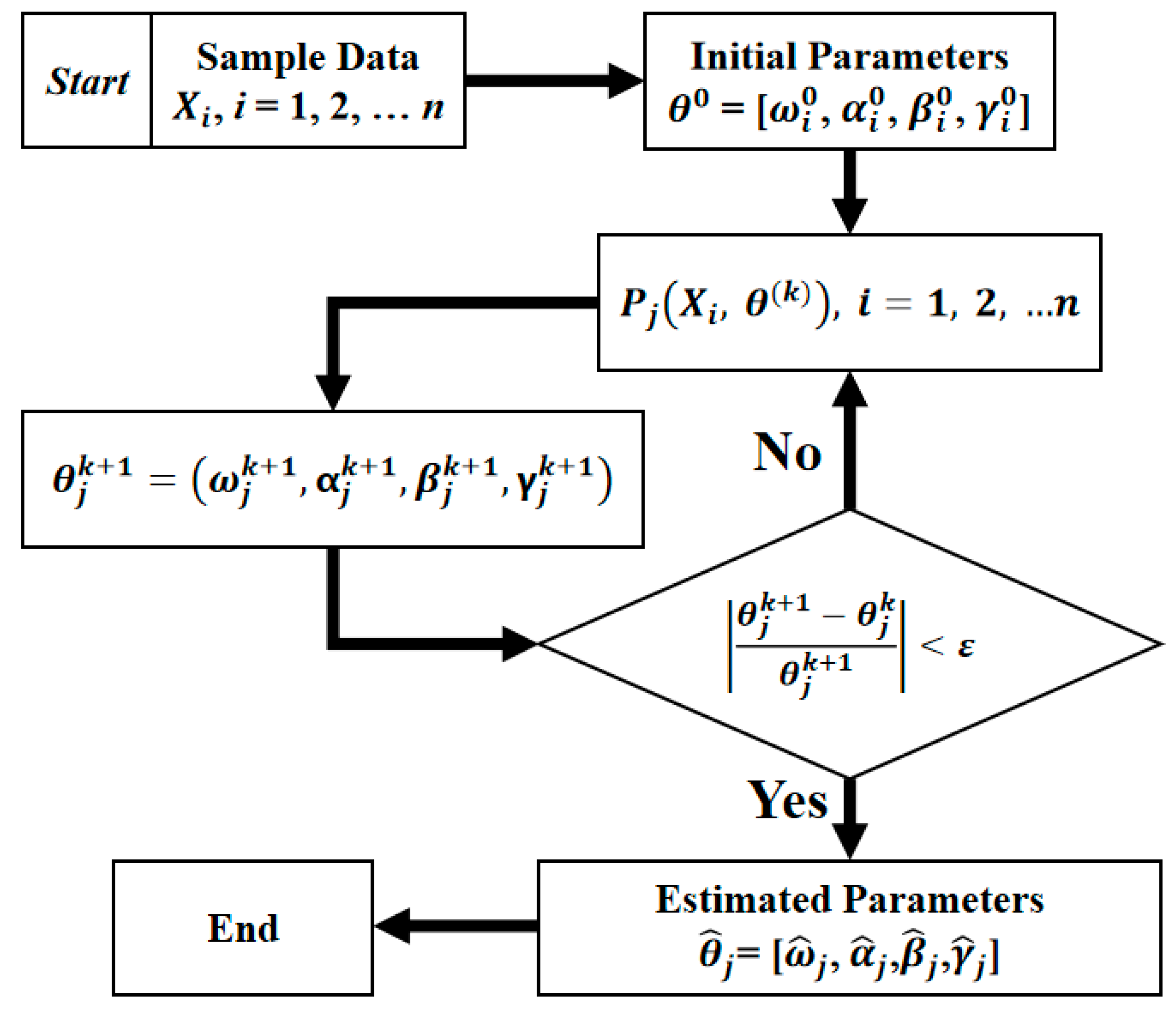
In this paper, we first estimated the two parameters of the mixed Weibull distribution model using the graph estimation method, and then solved the three parameter values of the single Weibull distribution using the maximum likelihood method, combined the estimates derived from the two methods to form the initial values of the EM iterative algorithm and iterated to solve them, and finally solved all parameter values of the mixed three-parameter model with the following flowchart shown in Figure 1:
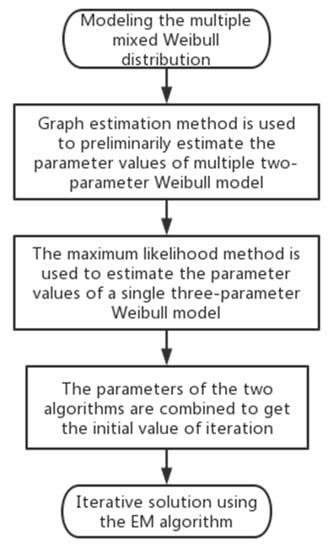
Figure 1.
Flow chart of the EM optimization algorithm for the hybrid Weibull model.
3. Three-Parameter Mixed WEIBULL Distribution Model Establishment
Assuming that a group of life test failure datapoints obeys the mixed Weibull distribution, this life test data can be considered as a total of m subgroup, and each subset has an independent failure mode and failure distribution, then the probability density of the total can be defined as:
where ; , , are the mixing weight, shape, scale, and location parameters of sub distribution i, respectively, and .
The failure probability distribution function of the system is given as follows:
The reliability (survivor) function of the mixture distribution is given as follows:
The failure rate of the mixture distribution is given as follows:
Each equation contains 4 m − 1 unknown parameters, and the evaluation of these parameters is a crucial step in modeling the mixed Weibull distribution.
4. Parameter Estimation Based on the EM Algorithm
4.1. Parameter Estimation Model of the EM Algorithm
The EM algorithm, first proposed by Dempester in 1977, aims to find a set of parameters that maximize the probability of occurrence of the target data, and is an effective method for solving optimization problems in the presence of hidden variables [25]. It can also complete the fitting of sample data even in the case of missing data. The specific steps of the EM algorithm are as follows:
Input: Observed variable data Y, hidden variable data Z, joint distribution ,
Output: Model parameters ;
- Select the initial values of the parameters and start the iteration;
- Step E: denote as the estimated value of the parameter of the ith iteration, and at the (i + 1)th iteration of step E, calculate
- Step M: Find the that maximizes and determine the estimate of the parameter for the (i + 1)th iteration
- Repeat step (2) and step (3) until convergence.
4.2. Solution by the EM Algorithm
According to the idea of EM algorithm, the hybrid Weibull distribution parameter estimation model can be established by the following steps in the case of known failure data:
where is the probability density function of a single three-parameter Weibull distribution and z is the observed failure data.
First introduce the hidden variables , , the stands for from , represents does not originate from .
4.2.1. Step E
Also, by the total probability formula
Therefore, we can get,
Substituting Equation (5) into Equation (6) yields
Then,
Substituting Equation (8) into Equation (7) yields
4.2.2. Step M
- Since the weight coefficients must add up to 1, it is necessary to introduce the Lagrange multiplier λ to bound ω, make , we can obtain
- Great likelihood of the probability density function yields
Substituting Equations (10)–(12) into , , yields
It can be seen that is a parameter related to , then the in the remaining two sets of equations can be replaced by , then we can obtain a set of equations , using MATLAB to solve the system of equations, solve the , and then bring in the equation for , the estimated values of the three parameters can be solved successively. The flow chart of this EM algorithm is shown in Figure 2.
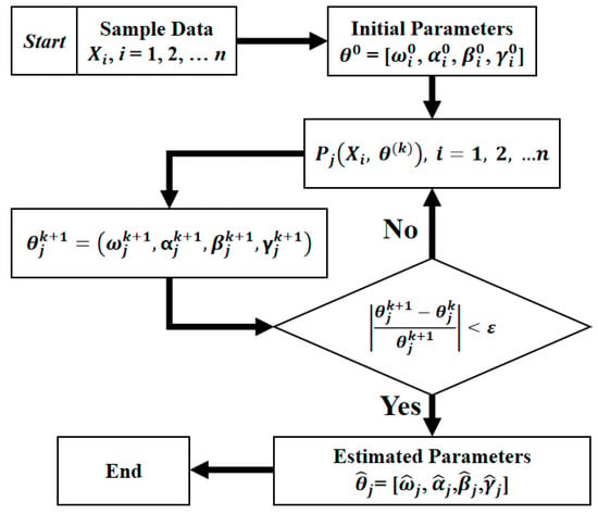
Figure 2.
Flow chart of the EM algorithm.
5. Instance Verification
5.1. m-Fold Weibull Distribution Simulation
The m-fold Weibull mixture model involves m sub-populations,
where is a weight coefficient and , are distribution functions either with two- or three-parameter Weibull distributions.
The Weibull distribution can be characterized as the distribution of a random variable W, such that the random variable
is the standard exponential distribution with intensity 1.
This implies that the Weibull distribution can also be characterized in terms of a uniform distribution. If U is uniformly distributed on (0,1), then the random variable is Weibull distributed with parameters k and . Note that here is equivalent to X just above. This leads to an easily implemented numerical scheme for simulating a Weibull distribution.
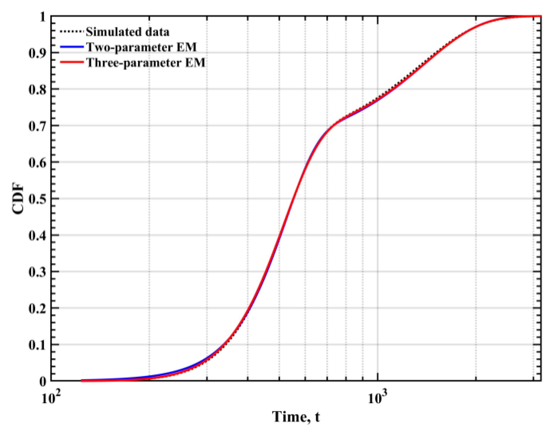
Based on the above method, we can simulate the Weibull distribution two-fold three-parameter random numbers, and then we can obtain the simulated Weibull distribution of the random numbers, and we fit this data with the two-parameter EM algorithm and three-parameter EM algorithm to obtain the fitted graph, see Figure 3. Please see Appendix A for the specific procedures written.
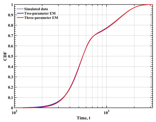
Figure 3.
Simulation of the cumulative distribution function of the mixed Weibull distribution.
The parameter estimates we obtained with different methods are shown in Table 1.

Table 1.
Simulation parameter estimation results.
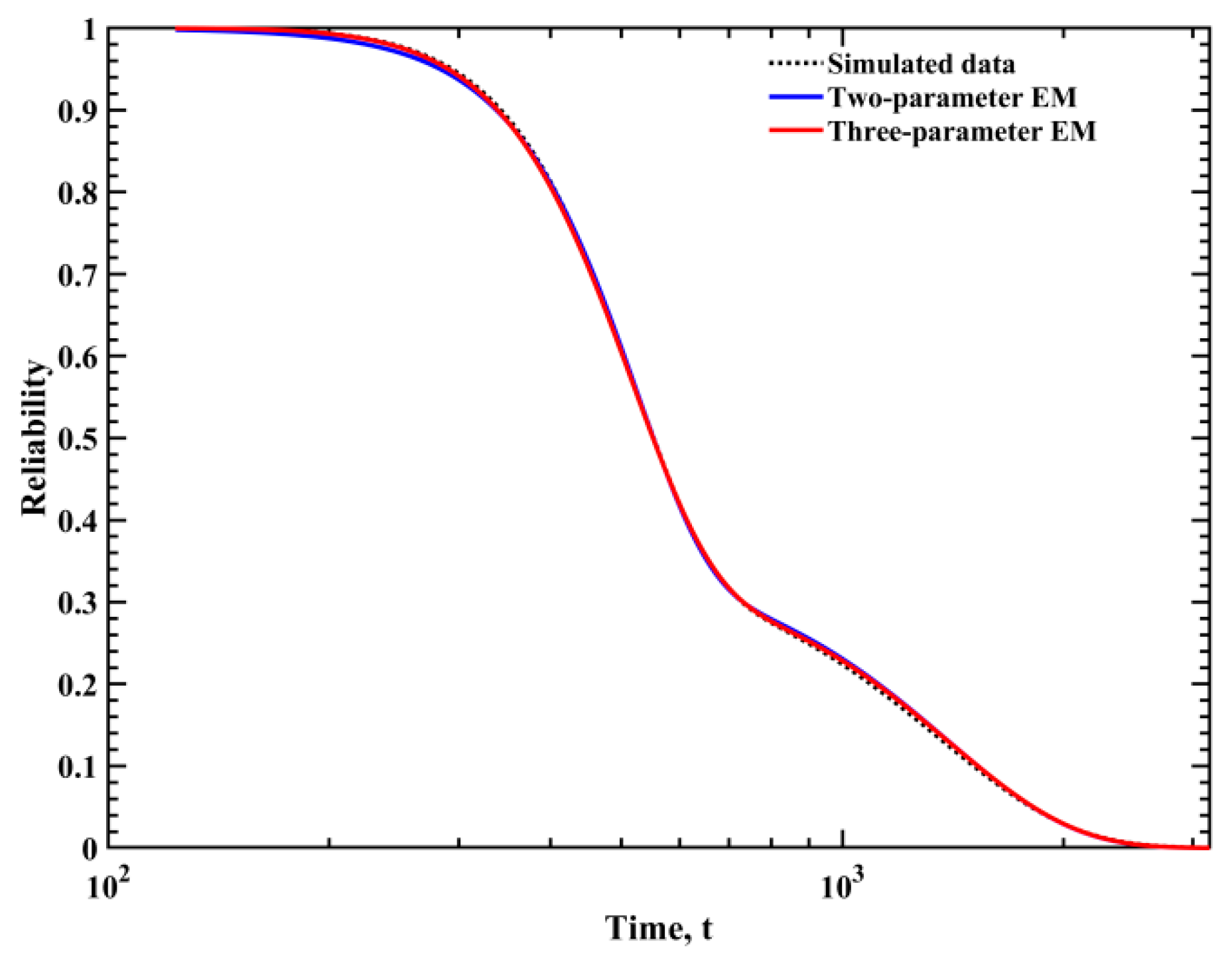
Based on the evaluation parameters derived from Table 1 and using Equations (2)–(4), we can obtain simulations of the probability density functions, reliability (survivor), and hazard functions of the mixture distributions by the two different methods, as illustrated in Figure 4, Figure 5 and Figure 6. We can deduce that the proposed method is the best fit.
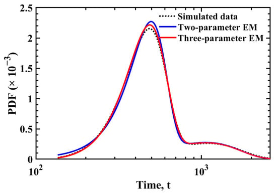
Figure 4.
Simulation of fitted probability density functions of failure times.
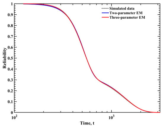
Figure 5.
Simulation of fitted reliability functions of failure times.
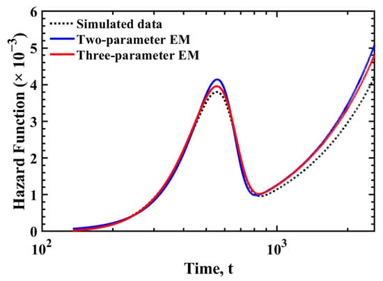
Figure 6.
Simulation of fitted hazard functions of failure times.
The merit of parameter estimation can be measured by the normalized root mean squared error (NRMSE) [26]. The normalized root mean squared error of the reliability estimate and the true value can be obtained from Equation (14):
Table 2 gives the NRMSE obtained from the parameter estimation by the above two methods.

Table 2.
Simulation of NRMSE results.
The NRMSE calculated by the proposed method was reduced by 0.0006 compared to the two-parameter EM algorithm in the simulation.
5.2. Application
5.2.1. Parameter Initial Value Selection and Fitting Results
To verify the validity of the method proposed in this paper, the sample data given in the literature [10] were used as an arithmetic example. In the selection of the initial values of η, β, and γ, γ has been directly set to 0 in some studies [7], which will greatly reduce the accuracy of the overall model calculation. Although the graph estimation method can roughly estimate the parameter values of the two-fold mixed Weibull model, its accuracy is not high, and only two parameters can be estimated, and the value of γ is set to zero. The maximum likelihood method can estimate three parameter values, but it can only be applied to a single Weibull distribution model. Therefore, in this paper, we combined the advantages of the two algorithms. The initial values η, β were obtained by the graph estimation method for the two-fold two-parameter Weibull distribution model, and the initial value γ was obtained by the maximum likelihood method for the single three-parameter Weibull distribution model measured on the same data. The sample data are shown in Table 3, which shows the number of failure cycles of a set of 60 appliances in one life test. We established the initial values based on this life sample as follows:

Table 3.
Failure data sample [10].
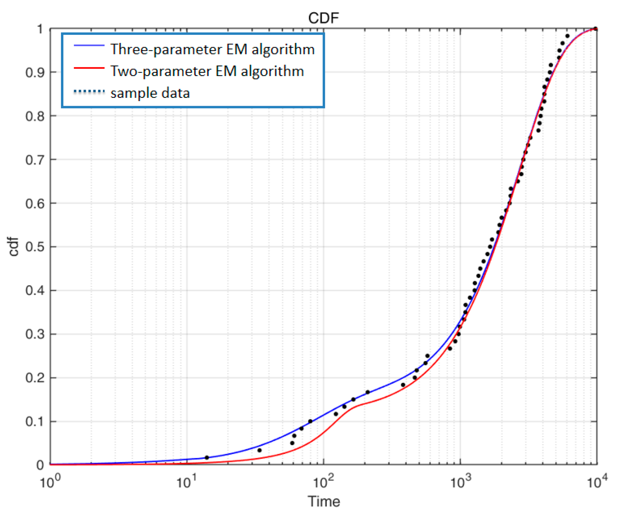
After obtaining the initial values, the EM algorithm proposed in this paper iteratively obtained the parameter estimates, weight estimates, and corresponding weight constraints of the mixed Weibull distribution model. The number of iterations was set to 10, and the obtained fitting curve is shown in Figure 7.
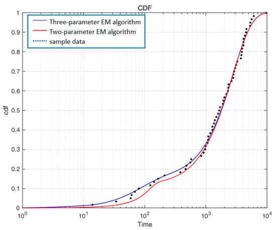
Figure 7.
Failure probability fitting curve of three-parameter mixed mode.
Table 4 gives a comparison of the parameter estimates corresponding to Figure 6 with those of several conventional algorithms from the literature [10]. It is easy to see that the three-parameter EM solver algorithm is more accurate and fits better than the two-parameter EM solver algorithm.

Table 4.
Comparison of parameter estimation results.
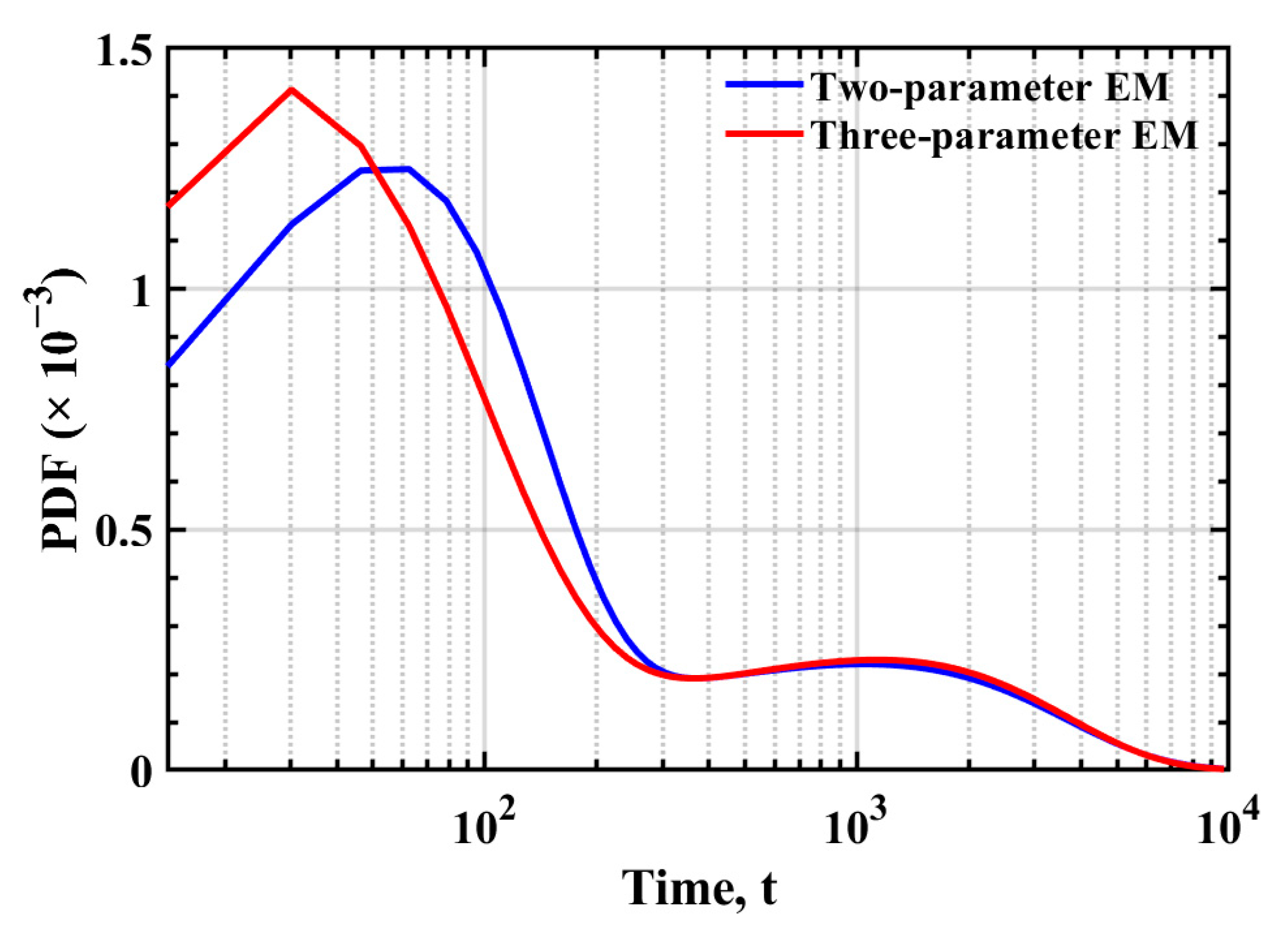
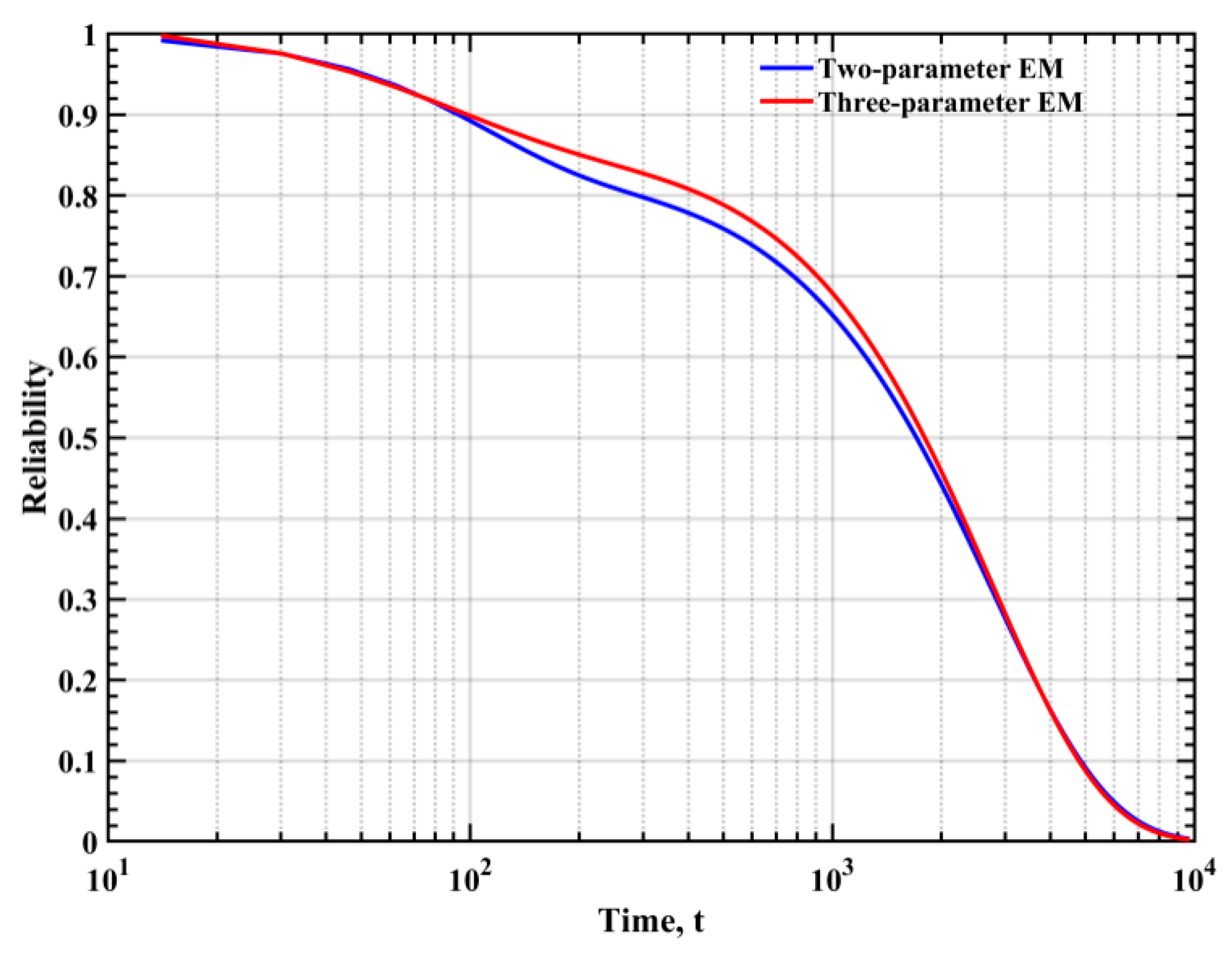
Based on the parameter estimates obtained in Table 3, we can obtain the probability density functions, reliability (survivor), and hazard functions of the mixture distributions by the two different methods, as illustrated in Figure 8, Figure 9 and Figure 10.
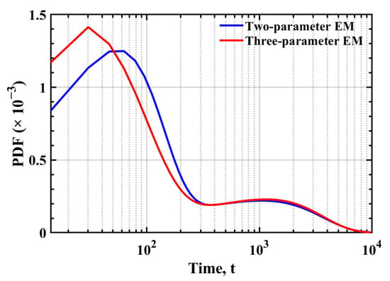
Figure 8.
Fitted probability density functions of failure times.
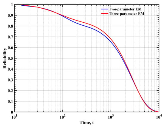
Figure 9.
Fitted reliability functions of failure times.
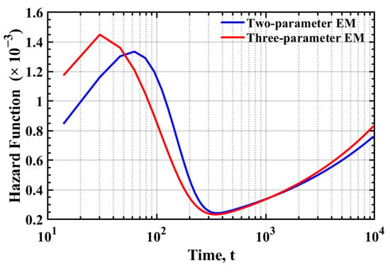
Figure 10.
Fitted hazard functions of failure times.
5.2.2. Goodness-of-Fit Test
The chi-square test, a very versatile hypothesis testing method, can count the degree of deviation between the actual observed value of the sample and the theoretical inferred value. Using the parameter estimates obtained by the method proposed in this paper, the chi-square test was performed at the significance level of .
here, F(t) is the two-fold failure probability distribution function shown in Equation (2), substituting the weight coefficients and parameter estimates into this equation and processing the batch of data according to the method shown in this equation. The original hypothesis H0 was that the sample data distribution obeys the double Weibull distribution of the parameter estimates in this paper.
Here, k represents the number of sample groups, is the frequency of each group, and denotes the expected sample size of the ith group under the original hypothesis H0; the calculations lead to
The results showed that the original hypothesis H0 was accepted.
We can still use the NRMSE method mentioned above to test the merits of the two fitted distribution curves and obtain the following results shown in Table 5.

Table 5.
NRMSE results.
The results showed that the NRMSE calculated by the proposed method was reduced by 0.0074 compared to the two-parameter EM algorithm.
5.3. Analysis of Results
In this paper, the parameter values of the two-fold Weibull distribution model were initially estimated by the graph estimation method, and the parameters of a single three-parameter Weibull distribution model were estimated by the maximum likelihood method. On this basis, the parameters of the two-fold three-parameter Weibull distribution model were estimated by the EM algorithm.
First, we conducted simulations for the mixed two-parameter EM algorithm and the mixed three-parameter EM algorithm, and we found that the mixed three-parameter EM algorithm had a smaller error and more accurate fitting than the mixed two-parameter EM algorithm by comparing their NRMSE. Then, we compared the graph estimation method and the two-fold two-parameter EM algorithm, and we found that the algorithm significantly improved in the accuracy of parameter estimation after only ten iterations. Moreover, the estimated value of the γ parameter could be accurately estimated, as shown in Table 4, which showed the effectiveness and accuracy of the algorithm. After the goodness-of-fit test, 95% of the test conditions were met, and the NRMSE was reduced by 0.0074 compared with the two-fold two-parameter EM algorithm. The proposed method can also be applied to the parameter estimation of a multiple three-parameter Weibull distribution.
The EM algorithm has the characteristic of introducing hidden variables. It is a very effective parameter estimation method in the case of missing samples, and it can complete the data model by adaptive iteration. Therefore, it is more accurate and effective in the case of small and large samples.
6. Conclusions
This paper proposed a parameter estimation method for the mixed three-parameter Weibull distribution based on the EM algorithm and designed an effective initial value selection method. The three parameters to be estimated and the weight coefficients in the mixed Weibull distribution could be solved by the method proposed in this paper. The obtained calculation results fit the sample data well, proving the proposed method’s effectiveness and superiority. The algorithm proposed in this paper had higher accuracy than the traditional algorithm and could obtain the location parameter γ more accurately.
Compared with the maximum likelihood method and graph estimation method, the form of hidden variables introduced by the optimization algorithm proposed in this paper was better able to perform adaptive iteration according to the sample data and obtain the parameter value that maximizes the probability of the group of sample data. The method is simple to understand and converges faster, avoiding the complicated process of solving beyond the equation.
The simulation results showed that the proposed method can fit the sample data very well, and the NRMSE results showed that the proposed method has a significant improvement in accuracy over the hybrid two-parameter EM algorithm.
Author Contributions
Conceptualization, Q.Z. and L.Z.; methodology, X.D.; validation, X.D. and R.Z.; formal analysis, X.D.; investigation, Q.Z.; data curation, X.D.; writing—original draft preparation, X.D.; writing—review and editing, F.S., F.X. and Z.L.; funding acquisition, L.Z. All authors have read and agreed to the published version of the manuscript.
Funding
This research was supported by National Natural Science Fund of China (No. 52005345, No. 52005344), National Key Research and Development Project (No.2020YFC2006701), Scientific Research Fund Project of Liaoning Provincial Department of Education (No. LFGD2020002), Major Project of the Ministry of Science and Technology of Liaoning Province (No.2022JH1/10400027), the National Natural Science Foundation of China (51975136, 52075109), the Science and Technology Innovative Research Team Program in Higher Educational Universities of Guangdong Province (2017KCXTD025), Special Research Projects in the Key Fields of Guangdong Higher Educational Universities (2019KZDZX1009), the Industry-University-Research Cooperation Key Project of Guangzhou Higher Educational Universities (202235139), and Guangzhou University Research Project (YJ2021002).
Institutional Review Board Statement
Not applicable.
Informed Consent Statement
Not applicable.
Data Availability Statement
Not applicable.
Acknowledgments
We thank the anonymous referees for their helpful comments that improved the quality of the manuscript.
Conflicts of Interest
The authors declare no conflict of interest.
Appendix A
code 1: application
clc; clear all; close all;
sc = get(groot,‘ScreenSize’);
%% load data.
Z = [14.0; 34; 59; 61; 69; 80; 123; 142; 165; 210; 381; 464; 479; 556; 574; 839; 917; 969; 991; …
1064; 1088; 1091; 1174; 1270; 1275; 1355; 1397; 1477; 1578; 1649; 1702; 1893; …
1932; 2001; 2161; 2292; 2326; 2337; 2628; 2785; 2811; 2886; 2993; 3122; 3248; 3715;
3790; 3857; 3912; 4100; 4106; 4116; 4315; 4510; 4584; 5267; 5299; 5583; 6065; 9701];
%% initialize params.
m = 2; % num of models.
theta = cell(m,1); % model parameters.
theta{1} = struct(‘w’, 0.1636, ‘alpha’, 105.6869, ‘beta’, 1.5276, ‘gamma’, 0.0); % weight alpha beta gamma
theta{2} = struct(‘w’, 0.8364, ‘alpha’, 2787.2, ‘beta’, 1.3576, ‘gamma’, 0.0); % weight alpha beta gamma
iters = 10;
[cd2P,wbT,wb2P,wbF2p,wbR2p,wbH2p] = weibullStd(Z,theta,’2P’);
theta = cell(m,1); % model parameters.
theta{1} = struct(‘w’, 0.2, ‘alpha’, 115.3, ‘beta’, 1.704, ‘gamma’, 3.4383); % weight alpha beta gamma
theta{2} = struct(‘w’, 0.8, ‘alpha’, 4511, ‘beta’, 1.733, ‘gamma’, 3.4384); % weight alpha beta gamma
[~,~,wb3P,wbF3p,wbR3p,wbH3p,theta3p] = weibullEM(Z,m,theta,iters,‘3P’);
figure;
scatter(Z, cd2P, 10, ‘ko’, ‘filled’);
hold on;
plot(wbT, wbF2p, ‘b’,wbT, wbF3p, ‘r’);
hold off;
set(gca,‘Xscale’,‘log’);
xlabel(‘Time, t’);
ylabel(‘CDF’);
grid on;
legend(‘Sample data’,‘Two-parameter EM’,‘Three-parameter EM’,‘Location’,‘northwest’);
print(‘paparCDF’,gcf,‘-r300’,‘-dtiffn’);
figure;
plot(wbT, wb2P*1000, ‘b’,wbT, wb3P*1000, ‘r’);
xlim([−500 10000]);
xlabel(‘Time, t’);
ylabel(‘PDF (× 10^{−3})’);
legend(‘Two-parameter EM’,‘Three-parameter EM’);
set(gca,‘Xscale’,‘log’);
grid on;
print(‘paparPDF’,gcf,‘-r300’,‘-dtiffn’);
figure;
plot(wbT, wbR2p, ‘b’,wbT, wbR3p, ‘r’);
xlabel(‘Time, t’);
ylabel(‘Reliability’);
legend(‘Two-parameter EM’,‘Three-parameter EM’);
set(gca,‘Xscale’,‘log’);
grid on;
print(‘paparReliability’,gcf,‘-r300’,‘-dtiffn’);
figure;
plot(wbT, wbH2p*1000, ‘b’,wbT, wbH3p*1000, ‘r’);
xlabel(‘Time, t’);
ylabel(‘Hazard Function (× 10^{−3})’);
legend(‘Two-parameter EM’,‘Three-parameter EM’);
set(gca,‘Xscale’,‘log’);
grid on;
print(‘paparHazard’,gcf,‘-r300’,‘-dtiffn’);
code 2:simulation
clc;clear;close all
% 三参数weibull
num = 1000;
eta1 = 1253;
beta1 = 2.25;
gamma1 = 125;
omega1 = 0.35;
eta2 = 438;
beta2 = 3.56;
gamma2 = 83;
grp1 = wblrnd3p(eta1,beta1,gamma1,1,omega1*num);
grp2 = wblrnd3p(eta2,beta2,gamma2,1,(1-omega1)*num);
[sgrp1,loc1] = sort(grp1);
[sgrp2,loc2] = sort(grp2);
frp1 = wblpdf3p(grp1,eta1,beta1,gamma1);
frp2 = wblpdf3p(grp2,eta2,beta2,gamma2);
% figure;
% plot(sgrp1,frp1(loc1),sgrp2,frp2(loc2),‘LineWidth’,1.5);
grp = [grp1,grp2];
[sgrp,sloc] = sort(grp);
%% initialize params.
m = 2; % num of models.
theta = cell(m,1); % model parameters.
theta{1} = struct(‘w’, 0.20, ‘alpha’, 1000, ‘beta’, 3.0, ‘gamma’, 0); % weight alpha beta gamma
theta{2} = struct(‘w’, 0.80, ‘alpha’, 450, ‘beta’, 2.9, ‘gamma’, 0); % weight alpha beta gamma
iters = 10;
[cd2P,wbT,wb2P,wbF2p,wbR2p,wbH2p,theta2p] = weibullEM(sgrp,m,theta,iters,‘2P’);
theta = cell(m,1); % model parameters.
theta{1} = struct(‘w’, 0.20, ‘alpha’, 1000, ‘beta’, 3.0, ‘gamma’, 100); % weight alpha beta gamma
theta{2} = struct(‘w’, 0.80, ‘alpha’, 450, ‘beta’, 2.9, ‘gamma’, 70); % weight alpha beta gamma
[~,~,wb3P,wbF3p,wbR3p,wbH3p,theta3p] = weibullEM(sgrp,m,theta,iters,‘3P’);
theta = cell(m,1); % model parameters.
theta{1} = struct(‘w’, 0.35, ‘alpha’, 1253, ‘beta’, 2.25, ‘gamma’, 125); % weight alpha beta gamma
theta{2} = struct(‘w’, 0.65, ‘alpha’, 438, ‘beta’, 3.56, ‘gamma’, 83); % weight alpha beta gamma
[cdP,~,wbPr,wbFr,wbRr,wbHr] = weibullStd(sgrp,theta,‘3P’);
figure;
plot(wbT, wbFr, ‘k:’, wbT, wbF2p, ‘b’, wbT, wbF3p, ‘r’);
set(gca,‘Xscale’,‘log’);
xlabel(‘Time, t’);
ylabel(‘CDF’);
grid on;
set(gca,‘Xscale’,‘log’);
legend(‘Simulated data’, ‘Two-parameter EM’,‘Three-parameter EM’,’Location’,’northwest’);
% print(‘SimulatedCDF’,gcf,‘-r300’,‘-dtiffn’);
figure;
plot(wbT, wbPr*1000, ‘k:’, wbT, wb2P*1000, ‘b’, wbT, wb3P*1000, ‘r’);
xlabel(‘Time, t’);
ylabel(‘PDF (× 10^{−3})’);
set(gca,‘Xscale’,’log’);
legend(‘Simulated data’, ‘Two-parameter EM’,‘Three-parameter EM’);
% print(‘SimulatedPDF’,gcf,‘-r300’,‘-dtiffn’);
figure;
plot(wbT, wbRr, ‘k:’,wbT, wbR2p, ‘b’, wbT, wbR3p, ‘r’);
xlabel(‘Time, t’);
ylabel(‘Reliability’);
set(gca,‘Xscale’,’log’);
legend(‘Simulated data’, ‘Two-parameter EM’,‘Three-parameter EM’);
% print(‘SimulatedReliability’,gcf,‘-r300’,‘-dtiffn’);
figure;
plot(wbT, wbHr*1000, ‘k:’, wbT, wbH2p*1000, ‘b’, wbT, wbH3p*1000, ‘r’);
xlabel(‘Time, t’);
ylabel(‘Hazard Function (× 10^{−3})’);
set(gca,‘Xscale’,’log’);
legend(‘Simulated data’, ‘Two-parameter EM’,‘Three-parameter EM’);
% print(‘SimulatedHazard’,gcf,‘-r300’,‘-dtiffn’);
References
- Jiang, W. Parameter estimation method of mixed weibull distribution in reliability analysis of aircraft% mixed Weibull distribution parameter estimation method. J. Eng. Des. 2015, 22, 26. [Google Scholar]
- Razali, A.M.; Al-Wakeel, A.A. Mixture Weibull distributions for fitting failure times data. Appl. Math. Comput. 2013, 219, 11358–11364. [Google Scholar] [CrossRef]
- Barraza-Contreras, J.M.; Piña-Monarrez, M.R.; Molina, A. Fatigue-life prediction of mechanical element by using the Weibull distribution. Appl. Sci. 2020, 10, 6384. [Google Scholar] [CrossRef]
- Wang, Y.; Peng, Z. Fatigue life prediction method of mechanical parts based on Weibull distribution. In IOP Conference Series: Materials Science and Engineering; IOP Publishing: Bristol, UK, 2020; Volume 782. [Google Scholar]
- Jiang, P.; Xing, Y.; Jia, X.; Guo, B. Weibull failure probability estimation based on zero-failure data. Math. Probl. Eng. 2015, 2015, 681232. [Google Scholar] [CrossRef]
- Cai, W.; Li, W.; Xu, J. Study on the PSN Curve of Sucker Rod Based on Three-Parameter Weibull Distribution. Materials 2022, 15, 560. [Google Scholar] [CrossRef]
- Ling, D.; Huang, H.Z.; Liu, Y. A method for parameter estimation of Mixed Weibull distribution. In Proceedings of the 2009 Annual Reliability and Maintainability Symposium, Fort Worth, TX, USA, 26–29 January 2009. [Google Scholar]
- Fajdiga, N.M. An improved algorithm for parameter estimation suitable for mixed Weibull distributions. Int. J. Fatigue 2000, 22, 75–80. [Google Scholar]
- Lu, Z.; Dong, L.; Zhou, J. Nonlinear least squares estimation for parameters of mixed Weibull distributions by using particle swarm optimization. IEEE Access 2019, 7, 60545–60554. [Google Scholar] [CrossRef]
- Elmahdy, E.E.; Aboutahoun, A.W. A new approach for parameter estimation of finite Weibull mixture distributions for reliability modeling. Appl. Math. Model. 2013, 37, 1800–1810. [Google Scholar] [CrossRef]
- Al-Baidhani, P.A.; Sinclair, C.D. Comparison of methods of estimation of parameters of the Weibull distribution. Commun. Stat. Simul. Comput. 1987, 16, 373–384. [Google Scholar] [CrossRef]
- Maqsood, A.; Aslam, M. A comparative study to estimate the parameters of mixed-Weibull distribution. Pakistan J. Stat. Op. Res. 2008, 4, 1–8. [Google Scholar] [CrossRef]
- Du, G.P.; He, L.D.; Zhang, B. Reliability modeling of electrical engineering products based on mixed Weibull distribution. Elect. Meas. Instrum. 2014, 51, 21–25. [Google Scholar]
- Jiang, R.; Murthy, D.N.P. Mixture of Weibull distributions—parametric characterization of failure rate function. Appl. Stoch. Models Data Anal. 1998, 14, 47–65. [Google Scholar] [CrossRef]
- Moeini, A.; Jenab, K.; Mohammadi, M.; Foumani, M. Fitting the three-parameter Weibull distribution with Cross Entropy. Appl. Math. Model. 2013, 37, 6354–6363. [Google Scholar] [CrossRef]
- Ismail, A.A. Estimating the parameters of Weibull distribution and the acceleration factor from hybrid partially accelerated life test. Appl. Math. Model. 2012, 36, 2920–2925. [Google Scholar] [CrossRef]
- Elmahdy, E.E. A new approach for Weibull modeling for reliability life data analysis. Appl. Math. Comput. 2015, 250, 708–720. [Google Scholar] [CrossRef]
- Zhang, L.; Jin, G.; You, Y. Reliability assessment for very few failure data and Weibull distribution. Math. Probl. Eng. 2019, 2019, 8947905. [Google Scholar] [CrossRef]
- Roldán-Nofuentes, J.A.; Regad, S.B. Comparison of the average kappa coefficients of two binary diagnostic tests with missing data. Mathematics 2021, 9, 2834. [Google Scholar] [CrossRef]
- Tsai, T.R.; Lio, Y.; Ting, W.C. Em algorithm for mixture distributions model with type-i hybrid censoring scheme. Mathematics 2021, 9, 2483. [Google Scholar] [CrossRef]
- Abd El-Raheem, A.E.R.M.; Hosny, M.; Abu-Moussa, M.H. On progressive censored competing risks data: Real data application and simulation study. Mathematics 2021, 9, 1805. [Google Scholar] [CrossRef]
- Lee, P.M. Bayesian Statistics An Introduction. J. Am. Stat. Assoc. 1990, 85, 128. [Google Scholar]
- Mclachlan, G.; Peel, D. Finite Mixture Models; Springer: New York, NY, USA, 2004. [Google Scholar]
- Mclachlan, G.J.; Krishnan, T. The EM Algorithm and Extensions. Biometrics 1998, 382, 260. [Google Scholar]
- Dempster, A.P. Maximum likelihood from incomplete data via the EM algorithm. J. R. Stat. Soc. 1977, 39, 1–22. [Google Scholar]
- Nocedal, J.; Wright, S.J. Numerical Optimization; Springer: Berlin, Germany, 1999. [Google Scholar]
Publisher’s Note: MDPI stays neutral with regard to jurisdictional claims in published maps and institutional affiliations. |
© 2022 by the authors. Licensee MDPI, Basel, Switzerland. This article is an open access article distributed under the terms and conditions of the Creative Commons Attribution (CC BY) license (https://creativecommons.org/licenses/by/4.0/).


