Article

Artificial Intelligence-Based Prediction of Crude Oil Prices Using Multiple Features under the Effect of Russia–Ukraine War and COVID-19 Pandemic

1
Department of Mechanical Engineering, University of Manitoba, Winnipeg, MB R3T 5V6, Canada
2
Computer Engineering Department, Technology Faculty, Sakarya University of Applied Sciences, Sakarya 54050, Turkey
3
Electrical and Electronics Engineering Department, Technology Faculty, Sakarya University of Applied Sciences, Sakarya 54050, Turkey
4
School of Aerospace Engineering, Beijing Institute of Technology, Beijing 100081, China
5
Department of Information Technology, Faculty of Computing and Information Technology, King Abdulaziz University, Jeddah 21589, Saudi Arabia
*
Author to whom correspondence should be addressed.
Mathematics 2022, 10(22), 4361; https://doi.org/10.3390/math10224361
Submission received: 28 October 2022 / Revised: 16 November 2022 / Accepted: 18 November 2022 / Published: 20 November 2022
(This article belongs to the Special Issue Application of Mathematical Methods in Financial Economics)

Abstract

:
The effect of the COVID-19 pandemic on crude oil prices just faded; at this moment, the Russia–Ukraine war brought a new crisis. In this paper, a new application is developed that predicts the change in crude oil prices by incorporating these two global effects. Unlike most existing studies, this work uses a dataset that involves data collected over twenty-two years and contains seven different features, such as crude oil opening, closing, intraday highest value, and intraday lowest value. This work applies cross-validation to predict the crude oil prices by using machine learning algorithms (support vector machine, linear regression, and rain forest) and deep learning algorithms (long short-term memory and bidirectional long short-term memory). The results obtained by machine learning and deep learning algorithms are compared. Lastly, the high-performance estimation can be achieved in this work with the average mean absolute error value over 0.3786.

1. Introduction

Crude oil is a significant energy source in the world [1]. The changes in crude oil prices have an important impact on the economic activities of countries all over the world. COVID-19 is a terrible disease, which quickly spread and heavily struck the world economy, health, and human life [2]. During this period, the crude oil price fluctuates greatly due to the global effects of the COVID-19 pandemic and Russia–Ukraine war. The severity of this fluctuation will increase as the supply and demand for oil and petroleum products change. Under this situation, predicting oil prices became crucial on a global scale.
There were some investigations focused on applying machine learning and deep learning to predict the prices of crude oil, Brent crude oil, and other commodities. These artificial intelligent methods are recognized to have powerful prediction capability, which were extensively developed and investigated during the last decades [3]. Deng et al. [1] proposed a deep transfer learning method based on the long short-term memory network (LSTM) to forecast Shanghai crude oil prices. Since the price was officially listed in March 2018, there is little available data on Shanghai crude oil prices. Therefore, the network is trained with Brent crude oil prices and the turned to Shanghai crude oil prices. A root mean square error (RMSE) value of 9.79 and a mean absolute error (MAE) value of 7.10 are obtained as the network performance.
Vo et al. [4] proposed the Brent oil price-bidirectional long short-term memory (BOP-BL) model to forecast oil prices based on bidirectional long short-term memory (Bi-LSTM). The proposed model is made up of two separate modules. The first module has three Bi-LSTM layers that support learning features in both forward and backward directions. The other module uses the fully connected layer and features extracted from the previous module to predict the oil price. Their method achieved the best prediction accuracy with an RMSE value of 1.55 and an MAE value of 1.2 by comparing with LSTM, convolutional neural network long short-term memory (CNN-LSTM), and convolutional neural network-bidirectional long short-term memory (CNN-Bi-LSTM) networks. Gabralla et al. [5] assessed the accuracy of daily West Texas Intermediate (WTI) crude oil price forecasting between 4 January 1999 and 10 October 2012. When making predictions, they compared the performance using three different machine learning algorithms with three, four, and five attributes. Kaymak et al. [6] proposed a model to predict the crude oil price fluctuations. Their model had the best results, with an MAE value of 0.5295, by comparing with artificial neural networks, the Fibonacci model, the golden ratio model, unoptimized values, and the support vector machine (SVM). Karasu et al. [7] proposed the chaotic Henry gas solubility optimization (CHGSO)-based LSTM model (CHGSO-LSTM) to solve the difficult problem of the crude oil price forecasting. Their model performed better with the particle swarm optimization long short-term memory (PSO-LSTM) model. Gupta et al. [8] proposed a crude oil price prediction model based on artificial neural networks. The proposed model had the best performance, with an RMSE value of 7.68. Busari et al. [9] compared AdaBoost-LSTM and AdaBoost-GRU models with LSTM and gated recurrent unit (GRU) models to predict crude oil prices. The AdaBoost-LSTM and AdaBoost-GRU models outperformed the LSTM and GRU models significantly. Yao et al. [10] used the LSTM and prophet algorithms to forecast crude oil prices. They found the prophet algorithm can produce the best prediction operations with an MAE value of 2.471.
Inspired by the above observations, this paper develops a new application that forecasts the change in crude oil prices by incorporating two global effects, the COVID-19 pandemic and the Russia–Ukraine war. As compared with most existing investigations, the main contributions of this work are threefold. (1) By using multiple features, current and long-dated datasets, and cross-validation in machine learning methods, the present results can achieve higher accuracy prediction. (2) By comparing machine learning and deep learning methods, the method that can produce the best results is determined. This matter is proven by comparing the results presented in this article with the results reported in the literature. (3) The effect of two major global crises, the COVID-19 pandemic and the Russia–Ukraine war, on crude oil prices is investigated in our study. Additionally, the major impact of these crises on crude oil price forecasting is discussed in detail.
The rest of this paper is organized as follows: In Section 2, the materials are provided and the artificial intelligence (AI) methods are briefly explained. In Section 3, the experimental results are given and the effects of global crises are interpreted with the results of machine learning and deep learning. Lastly, in Section 4, the conclusions of this work are presented.

2. Material and Methods

2.1. Artificial Intelligence Methods

In many data processing and big data problems, AI methods are widely used for classification [11], clustering [12], detection [13], and prediction [14,15]. AI is a broad term that encompasses a variety of techniques, including fuzzy methods [16], neural network-based algorithms [17], heuristic algorithms [18], machine learning [19], and deep learning [20]. This study focuses on the prediction of crude oil data and the results obtained using machine learning and deep learning methods are compared.
Three machine learning methods with excellent performance are employed in this work. These methods are SVM, linear regression (LR), and rain forest (RF). SVM is a classification algorithm based on statistical learning [21]. The SVM is initially developed as a method for solving two-class linear data classification problems and later evolved into a method for solving both nonlinear and multiple data classification problems. Essentially, the objective of SVM is to create a hyperplane that separates the classes in the most effective way [21,22].
LR is a machine learning algorithm that predicts a quantitative variable using one or more independent features in a linear fashion [23]. The independent variable has one or more features that can be used to estimate the dependent variable. More independent variables can be adopted to estimate the coefficients of the linear equation to better predict the algorithm-dependent variable value.
RF is a classification algorithm that employs a set of decision trees for predictions [24,25,26,27]. The RF attracted much attention owing to its advantages of high speed and excellent performance in classifications [28,29].
Cross-validation is a method for evaluating the performance of machine learning models accurately [21]. In this work, the five-fold cross-validation process shown in Figure 1 was integrated with the machine learning algorithms to improve performance, prevent overfitting, and ensure accurate prediction [30]. Meanwhile, the cross-validation can also reduce the training times and thus the results can be obtained efficiently.
Two deep learning methods with excellent performance are employed in this work. These methods are LSTM and Bi-LSTM. LSTM is a recurrent neural network (RNN) architecture that remembers values at random time intervals. The LSTM is widely used to classify, process, and predict time series with unknown time delays [31,32]. In this study, many different parameters were tested and the LSTM network, where the best performance was obtained, was used. Table 1 and Table 2 show LSTM and Bi-LSTM architecture. Only the “Bidirectional (LSTM)” layers on the architecture was used as the “LSTM” layer in the LSTM network. The number of train epochs for both models was fixed by 70 iterations. The first layer of the LSTM network used is the input layer. The number of steps of this layer is 5507 and the number of blocks is 8. The input and output of the input layer take the same values. The input value of the next layer is the same as the output value. While the number of steps of this layer is 5507, the number of blocks is 128. In the next layer, while the number of steps remains the same, the number of blocks is set to 256. The next layer is the dropout layer, and the output of the LSTM layer that it is connected to has the same values as the input and output of the dropout layer. The LSTM layer, which is the layer before the last layer, has the same input as the output of the previous LSTM layer, but there is no step value in its output. The last layer is the dense layer. Its input is the same as the output of the previous layer, but the number of blocks is set to 1.
Bi-LSTM is a combination of two independent RNNs. This structure ensures the network has the backward and forward-looking information about the sequence at each time step. Different from LSTM, Bi-LSTM runs the system inputs in two directions, one from past to future and the other from future to past, which protects information from the future and combines two hidden states [32]. In this study, many different parameters were tested and the Bi-LSTM network with the best performance was used. The first layer of the Bi-LSTM network used is the input layer. The number of steps of this layer is 5507 and the number of blocks is 4. The input and output of the input layer take the same values. The input value of the next layer is the same as the output value. While the number of steps of this layer is 5507, the number of blocks is 64. In the next layer, while the number of steps remains the same, the number of blocks is set to 128. The next layer is the dropout layer, and the output of the LSTM layer it is connected to has the same values as the input and output of the dropout layer. The Bi-LSTM layer, which is the layer before the last layer, has the same input as the output of the previous LSTM layer, but there is no step value in its output. The last layer is the dense layer. Its input is the same as the output of the previous layer, but the number of blocks is set to 1.

2.2. Performance Metrics

Mean absolute error (MAE) and mean squared error (MSE) are selected as the performance matrices in this work. MAE is a performance metric that is calculated by averaging absolute error values. The MAE can be calculated as [33]:
M A E = 1 a i = 1 a | A C T P R E D |
where A C T is the actual value and P R E D is the predicted value. MAE stands for the sum of the absolute values of the differences between the actual and estimated values.
MSE is a performance metric that is calculated by squaring error values. The MSE can be calculated as [34]:
M S E = 1 a i = 1 a ( A C T P R E D ) 2
where A C T is the actual value and P R E D is the predicted value. MAE stands for the sum of the squares of the differences between the actual and estimated values.

2.3. Dataset

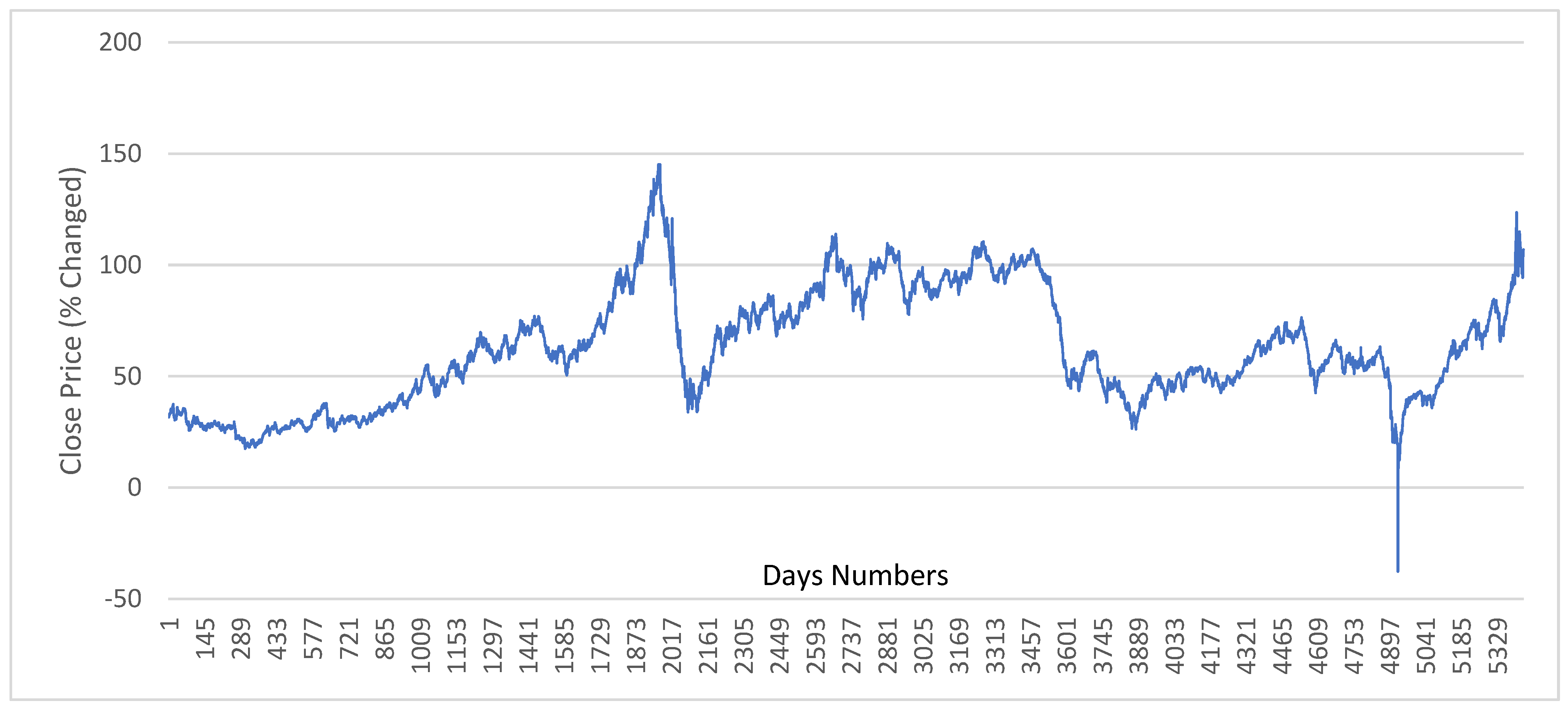
The crude oil data used in this work are obtained from Yahoo Finance [35] and recorded between 2000 and 2022 and used as the dataset. This dataset includes the crude oil opening, closing, highest, and lowest prices, adjusted close price (adjusted close price means adjusted price for dividend and/or capital gain distributions) and volume data, as the features of dataset, which are described as multiple features. All these features are included in the dataset as a separate column. All the features, except the closing price are used as input in the used machine learning and deep learning methods. All data used here are used as raw data and no pre-processing or feature extraction is applied. Each column contains 5460 records. As a result, a total number of 32,760 records are utilized for training and testing procedures. The closing prices of crude oil are estimated in this work by using the described dataset. Figure 2 shows a graphical representation of the closing values in the dataset. In other words, Figure 2 depicts the appearance of the dataset that will be estimated.

2.4. The Proposed Method

The flow diagram of the method proposed in this study that performs prediction with high performance is shown in Figure 3. With this method, firstly, the data set is obtained automatically from the Yahoo Finance source. Then, the features to be used in the prediction process are determined. Data segmentation is performed for training and testing processes over the specified features. After pre-processing is performed to extract problematic data, such as empty values, it is selected whether to apply the cross-validation process in the estimation process.
If cross-validation is to be applied, selection of fold is made and then the estimation method (RF, LR, SVM, LSTM, and Bi-LSTM) is selected. If cross-validation will not be made, the direct estimation method is selected. Training is conducted according to the chosen method and the results are tested. After the test process, performance results are obtained with MAE and MSE methods.

3. Experimental Results

The main goal of this work is to reveal changes in crude oil prices caused by the global effects of the COVID-19 pandemic and the Russia–Ukraine war by using a long-term and multi-featured dataset and a prediction application. Machine learning and deep learning are used as AI methods in this work. Machine learning methods, including SVM, LR, and RF, and deep learning methods, including LSTM and Bi-LSTM suitable for time series, are employed.
The train and test data are carefully selected to depict the effects of the COVID-19 pandemic and the Russia–Ukraine war. As a result, the test data are determined to be the previous two months, four months, eight months, sixteen months, and thirty-two months, with May 2022 as the deadline. The data from the first two months of the Russia–Ukraine war are involved in the training of that for the last two months, with the goal of monitoring the effects in the next two months. Figure 4 depicts the results for the previous two months. As shown in Figure 4, the results obtained using machine learning methods and their corrected results using five-fold cross-validation are very close to the real values. Since the effect of war is accounted in the training data, the estimation results of the methods were tracking the real values for the past two months. For the other experimental results, the situations are different (four, eight, sixteen, and thirty-two months).
When the data of the last four months are mentioned, the goal is to obtain results for a situation that the effects of the pandemic slowed, and the war did not yet begin. The application without data from the war period in the training in Figure 5 diverges from the real values after the start of the war. It clearly indicates the effect of the Russia–Ukraine war on oil prices, but also demonstrates that omitting data from such crisis processes has a direct impact on the accuracy of the forecasting results. This is also seen in the MAE and MSE values given in Figure 5. As can be seen in Figure 5, there are significant differences in the MAE and MSE values in the predictions made before and after the start of the war (red line). These results clearly show the impact of the war on crude oil prices.
Using the data from the previous eight months, another experimental study was conducted. This data include a period when the world economies gradually began to recover from the effects of the pandemic at the end of the last two years. Figure 6 shows the results of the application that was run with these data. Because the pandemic data were involved in the training, the estimated results during the pandemic period are very close to the real values. Moreover, because the data from the Russia–Ukraine war period were not included in the training, the estimation results after the start of the war began to diverge from the real values. As previously stated, the impact of the war can also be found here.
The prediction operation is performed using data from the previous sixteen months in another experimental study, and the results are shown in Figure 7. Since the first year of data from the COVID-19 pandemic is incorporated into the training process, the results are close to the real values until the war broke out. It can be clearly seen that after the start of the war, the estimated values diverged from the actual values as well.
The prediction is made using data from the previous thirty-two months as in the previous experimental study and the results are shown in Figure 8. The experimental results in this case are obtained by training without using the pandemic data. As shown in the graph, the predictions made during the sharp drop in crude oil prices that occurred by closure period, which began shortly after the start of the pandemic and ended with negative values, cannot fully reflect the real values. Particularly, for SVM and RF algorithms, we are unable to predict negative values and make a reverse prediction. This situation is depicted in Figure 8. Sudden changes caused by a global crisis, such as COVID-19, pose a major challenge to the application of forecasting. Furthermore, the estimated results after the start of the war show a divergence from the real values.
It is impossible to say whether the cross-validation process used for all methods in all graphs shown in Figure 4, Figure 5, Figure 6, Figure 7 and Figure 8 makes a visual difference. Table 3 shows the MAE and MSE values of the prediction results to show the effect of cross-validation as well as the methods used. To make a better understanding, the numerical results in Table 3 are also graphically presented in Figure 9 and Figure 10.
The RF algorithm without cross-validation obtained for thirty-two months can achieve the best performance in MAE results and the RF algorithm without cross-validation obtained for sixteen months can achieve the best performance in MSE results. The results of the LR algorithm, which correctly estimate the negative peak value in Figure 9 for thirty-two months of data, are acceptable and considered to perform well. Moreover, the results show that cross-validation processes in SVM and LR algorithms perform slightly better. The RF algorithm produces slightly worse results. Therefore, it can be concluded that cross-validation is ineffective in this application.
When all the results and graphics are considered together, it is clearly seen that the predictions made by including global crises in the training data produce better results. Moreover, as the estimation periods lengthen, the accuracy of the results improves. The reason is that long-term forecasts are less affected by the divergences that occurred during the Russia–Ukraine war. This demonstrates how events that directly affect the supply balance; for instance, the war causes price volatility and makes forecasting difficult. Another conclusion is that price drops, which occurred early in the pandemic and reached negative values, became a difficult-to-predict problem because they diverged the price trend from its normal path. As a result, for this situation, the MSE values in Table 3 and Figure 10 are quite high.
As can be seen in Table 3 and Figure 10, (except for the results of 16 months and 32 months in the results of SVM) long-term forecasts give better results than shorter-term forecasts. In fact, the error is expected to be higher for longer-term forecasts under normal conditions. However, the increase in errors as the estimation period shortens in this study shows that the global crisis has an effect on crude oil prices.
In addition to machine learning, another AI learning method, a deep learning application is also considered. LSTM and Bi-LSTM models, which are deep learning methods with effective use in time series, are used in this work. Table 4 shows the results for these models using the same dataset for the same time periods.
From Table 4, it is obvious that the obtained results are inferior to those obtained by using the machine learning methods in Table 3. Consequently, it can be determined that the used machine learning methods outperform LSTM and Bi-LSTM models in terms of the dataset and problem studied.
Another focus of the research is improving the prediction performance through the use of long-term and multi-featured data. In Table 5, comparisons are made with studies performed on different data sets and with different ML/DL algorithms. In this study, it is seen that both ML and DL results obtained by using long-term/big datasets and multiple features are better than other studies. It is not difficult to find that the results of the three different machine learning algorithms presented in this work outperform those in other literature. It is regarded as a major contribution of this work, as compared with other studies. The good results obtained here do not necessarily indicate the poor performance of the methods presented in other studies. It shows that the use of a long-term dataset and multiple features improves performance, as this study focuses on.

4. Conclusions

In this work, the effects of global crises, such as COVID-19 and the Russia–Ukraine war, on crude oil prices are investigated by using AI algorithms. We compare the results obtained by machine learning and deep learning algorithms comprehensively. The high-performance estimation can be achieved with the average mean absolute error value over 0.3786. As a result, the abrupt fluctuations that occurred since the start of the global crises have a negative impact on data prediction accuracy. In addition to the effects of global crises, another focus of this work is finding that crude oil prices can be predicted more accurately by using long-term and multi-featured data as another focal point. When compared with the previous studies, it was discovered that the present results are superior. The relationship between cross-validation and prediction performance is also discussed in this research. According to the results, the use of cross-validation does not have a major impact on obtaining more accurate crude oil price prediction data.
As a limitation, it can be costly to train machine learning algorithms using large and complex data models. Extensive hardware is also required to do complicated mathematical calculations. However, there are different methods for effective use of CPU and GPU resources for data preprocessing and training, which can significantly reduce calculation costs and time. One of these methods is the overlap of data preprocessing and model training. Data preprocessing is performed one step ahead of training, which helps to reduce the overall training time for the model. Additionally, in this study, an ML method was identified that accurately predicts the long-term price of crude oil. Therefore, to reduce time and calculation costs, we should only rely on the final proposed method and the other studied methods can be disregarded. It is believed that the workload and complexity will be manageable, given this strategy. In this regard, a very cost-effective and balanced model was introduced.
In future works, we plan to develop DL networks for more accurate predictions. Additionally, the neuro-fuzzy inference system (ANFIS) is one of the methods where its inference system is a set by fuzzy rules with the potential to learn. This algorithm, along with other algorithms, such as teaching–learning-based optimization (TLBO), should be considered as algorithms that can help improve prediction. In this regard, in future works, we will implement these algorithms and use them to compare the results.

Author Contributions

Conceptualization, H.J., S.U., S.K., Q.Y. and M.O.A.; methodology, H.J., S.U., S.K., Q.Y. and M.O.A.; software, H.J., S.U., S.K., Q.Y. and M.O.A.; validation, H.J., S.U., S.K., Q.Y. and M.O.A.; formal analysis, H.J., S.U., S.K., Q.Y. and M.O.A.; investigation, H.J., S.U., S.K., Q.Y. and M.O.A.; writing—original draft preparation, H.J., S.U., S.K., Q.Y. and M.O.A.; writing—review and editing, H.J., S.U., S.K., Q.Y. and M.O.A.; supervision, H.J., S.U., S.K., Q.Y. and M.O.A. All authors have read and agreed to the published version of the manuscript.

Funding

This research work was funded by Institutional Fund Projects under Grant no. (IFPDP-226-22). Therefore, the authors gratefully acknowledge technical and financial support from the Ministry of Education and King Abdulaziz University (KAU), Jeddah, Saudi Arabia.

Data Availability Statement

Not applicable.

Acknowledgments

This research work was funded by Institutional Fund Projects under Grant no. (IFPDP-226-22). Therefore, the authors gratefully acknowledge technical and financial support from the Ministry of Education and King Abdulaziz University (KAU), Jeddah, Saudi Arabia.

Conflicts of Interest

The authors declare no conflict of interest.

References

  1. Deng, C.; Ma, L.; Zeng, T. Crude Oil Price Forecast Based on Deep Transfer Learning: Shanghai Crude Oil as an Example. Sustainability 2021, 13, 13770. [Google Scholar] [CrossRef]
  2. Sabah, N.; Sagheer, A.; Dawood, O. Blockchain-based solution for COVID-19 and smart contract healthcare certification. Iraqi J. Comput. Sci. Math. 2021, 2, 1–8. [Google Scholar] [CrossRef]
  3. Aggarwal, K.; Mijwil, M.M.; Sonia; Al-Mistarehi, A.-H.; Alomari, S.; Gök, M.; Alaabdin, A.M.Z.; Abdulrhman, S.H. Has the future started? The current growth of artificial intelligence, machine learning, and deep learning. Iraqi J. Comput. Sci. Math. 2022, 3, 115–123. [Google Scholar]
  4. Vo, A.H.; Nguyen, T.; Le, T. Brent oil price prediction using Bi-LSTM network. Intell. Autom. Soft Comput. 2020, 26, 1307–1317. [Google Scholar] [CrossRef]
  5. Gabralla, L.A.; Jammazi, R.; Abraham, A. Oil Price Prediction Using Ensemble Machine Learning. Proceeding of the International Conference on Computing, Electrical and Electronic Engineering (ICCEEE), Khartoum, Sudan, 26–28 August 2013; pp. 674–679. [Google Scholar]
  6. Kaymak, Ö.Ö.; Kaymak, Y. Prediction of crude oil prices in COVID-19 outbreak using real data. Chaos Solitons Fractals 2022, 158, 111990. [Google Scholar] [CrossRef]
  7. Karasu, S.; Altan, A. Crude oil time series prediction model based on LSTM network with chaotic Henry gas solubility optimization. Energy 2022, 242, 122964. [Google Scholar] [CrossRef]
  8. Gupta, N.; Nigam, S. Crude oil price prediction using artificial neural network. Procedia Comput. Sci. 2020, 170, 642–647. [Google Scholar] [CrossRef]
  9. Busari, G.A.; Lim, D.H. Crude oil price prediction: A comparison between AdaBoost-LSTM and AdaBoost-GRU for improving forecasting performance. Comput. Chem. Eng. 2021, 155, 107513. [Google Scholar] [CrossRef]
  10. Yao, L.; Pu, Y.; Qiu, B. Prediction of Oil Price Using LSTM and Prophet. Proceeding of the International Conference on Applied Energy, Bangkok, Thailand, 29 November–2 December 2021. [Google Scholar]
  11. Mukhamediev, R.I.; Popova, Y.; Kuchin, Y.; Zaitseva, E.; Kalimoldayev, A.; Symagulov, A.; Levashenko, V.; Abdoldina, F.; Gopejenko, V.; Yakunin, K.; et al. Review of Artificial Intelligence and Machine Learning Technologies: Classification, Restrictions, Opportunities and Challenges. Mathematics 2022, 10, 2552. [Google Scholar] [CrossRef]
  12. Ezugwu, A.E.; Ikotun, A.M.; Oyelade, O.O.; Abualigah, L.; Agushaka, J.O.; Eke, I.C.; Akinyelu, A.A. A comprehensive survey of clustering algorithms: State-of-the-art machine learning applications, taxonomy, challenges, and future research prospects. Eng. Appl. Artif. Intell. 2022, 110, 104743. [Google Scholar] [CrossRef]
  13. Nassif, A.B.; Talib, M.A.; Nasir, Q.; Afadar, Y.; Elgendy, O. Breast cancer detection using artificial intelligence techniques: A systematic literature review. Artif. Intell. Med. 2022, 110, 102276. [Google Scholar] [CrossRef] [PubMed]
  14. Wang, C.-N.; Yang, F.-C.; Nguyen, V.T.T.; Vo, N.T.M. CFD Analysis and Optimum Design for a Centrifugal Pump Using an Effectively Artificial Intelligent Algorithm. Micromachines 2022, 13, 1208. [Google Scholar] [CrossRef] [PubMed]
  15. Dhakal, A.; McKay, C.; Tanner, J.J.; Cheng, J. Artificial intelligence in the prediction of protein–ligand interactions: Recent advances and future directions. Brief. Bioinform. 2022, 23, bbab476. [Google Scholar] [CrossRef] [PubMed]
  16. Nguyen, T.V.T.; Huynh, N.T.; Vu, N.C.; Kieu, V.N.D.; Huang, S.C. Optimizing compliant gripper mechanism design by employing an effective bi-algorithm: Fuzzy logic and AN-FIS. Microsyst. Technol. 2021, 27, 3389–3412. [Google Scholar] [CrossRef]
  17. Kabeya, Y.; Okubo, M.; Yonezawa, S.; Nakano, H.; Inoue, M.; Ogasawara, M.; Saito, Y.; Tanboon, J.; Indrawati, L.A.; Kumutpongpanich, T.; et al. Deep convolutional neural network-based algorithm for muscle biopsy diagnosis. Lab. Investig. 2022, 102, 220–226. [Google Scholar] [CrossRef]
  18. Yuan, J.; Zhao, M.; Esmaeili-Falak, M. A comparative study on predicting the rapid chloride permeability of self-compacting concrete using meta-heuristic algorithm and artificial intelligence techniques. Struct. Concr. 2022, 23, 753–774. [Google Scholar] [CrossRef]
  19. Ismail, L.; Materwala, H.; Tayefi, M.; Ngo, P.; Karduck, A.P. Type 2 Diabetes with Artificial Intelligence Machine Learning: Methods and Evaluation. Arch. Comput. Methods Eng. 2022, 29, 313–333. [Google Scholar] [CrossRef]
  20. Sujith, A.V.L.N.; Sajja, G.S.; Mahalakshmi, V.; Nuhmani, S.; Prasanalakshmi, B. Systematic review of smart health monitoring using deep learning and Artificial intelligence. Neurosci. Inform. 2022, 2, 100028. [Google Scholar] [CrossRef]
  21. Cortes, V.; Cortes, C.; Vapnik, V. Support-vector networks. Mach. Learn. 1995, 20, 273–297. [Google Scholar] [CrossRef]
  22. Petridis, K.; Tampakoudis, I.; Drogalas, G.; Kiosses, N. A Support Vector Machine model for classification of efficiency: An application to M&A. Res. Int. Bus. Financ. 2022, 61, 101633. [Google Scholar]
  23. Gupta, I.; Mittal, H.; Rikhari, D.; Singh, A.K. MLRM: A Multiple Linear Regression based Model for Average Temperature Prediction of A Day. arXiv 2022, preprint. arXiv:2203.05835. [Google Scholar]
  24. Azar, A.T.; Elshazly, H.I.; Hassanien, A.E.; Elkorany, A.M. A random forest classifier for lymph diseases. Comput. Methods Programs Biomed. 2014, 113, 465–473. [Google Scholar] [CrossRef] [PubMed]
  25. Breiman, L. Random forests. Mach. Learn. 2001, 45, 5–32. [Google Scholar] [CrossRef]
  26. Amit, Y.; Geman, D. Shape quantization and recognition with randomized trees. Neural Comput. 1997, 9, 1545–1588. [Google Scholar] [CrossRef] [Green Version]
  27. Ho, T.K. Random decision forests. In Proceedings of the 3rd International Conference on Document Analysis and Recognition, Montreal, QC, Canada, 14–16 August 1995. [Google Scholar]
  28. Pal, M. Random forest classifier for remote sensing classification. Int. J. Remote Sens. 2005, 26, 217–222. [Google Scholar] [CrossRef]
  29. Belgiu, M.; Drăguţ, L. Random forest in remote sensing: A review of applications and future directions. ISPRS J. Photogramm. Remote Sens. 2016, 114, 24–31. [Google Scholar] [CrossRef]
  30. Cheng, J.; Kuang, H.; Zhao, Q.; Wang, Y.; Xu, L.; Liu, J.; Wang, J. DWT-CV: Dense weight transfer-based cross validation strategy for model selection in biomedical data analysis. Future Gener. Comput. Syst. 2022, 135, 20–29. [Google Scholar] [CrossRef]
  31. Smagulova, K.; James, A.P. A survey on LSTM memristive neural network architectures and applications. Eur. Phys. J. Spec. Top. 2019, 228, 2313–2324. [Google Scholar] [CrossRef]
  32. Khullar, S.; Singh, N. Water quality assessment of a river using deep learning Bi-LSTM methodology: Forecasting and validation. Environ. Sci. Pollut. Res. 2022, 29, 12875–12889. [Google Scholar] [CrossRef]
  33. Graves, A.; Fernández, S.; Schmidhuber, J. Bidirectional LSTM networks for improved phoneme classification and recognition. In International conference on artificial neural networks; Springer: Berlin/Heidelberg, Germany, 2005; Volume 3697, pp. 799–804. [Google Scholar]
  34. Shaik, N.B.; Pedapati, S.R.; Othman, A.R.; Bingi, K.; Dzubir, F.A.A. An intelligent model to predict the life condition of crude oil pipelines using artificial neural networks. Neural Comput. Appl. 2021, 33, 14771–14792. [Google Scholar] [CrossRef]
  35. Crude Oil Jul 22 (CL=F) Stock Historical Prices & Data—Yahoo Finance. Available online: https://finance.yahoo.com/quote/CL%3DF/history?p=CL%3DF (accessed on 3 June 2022).
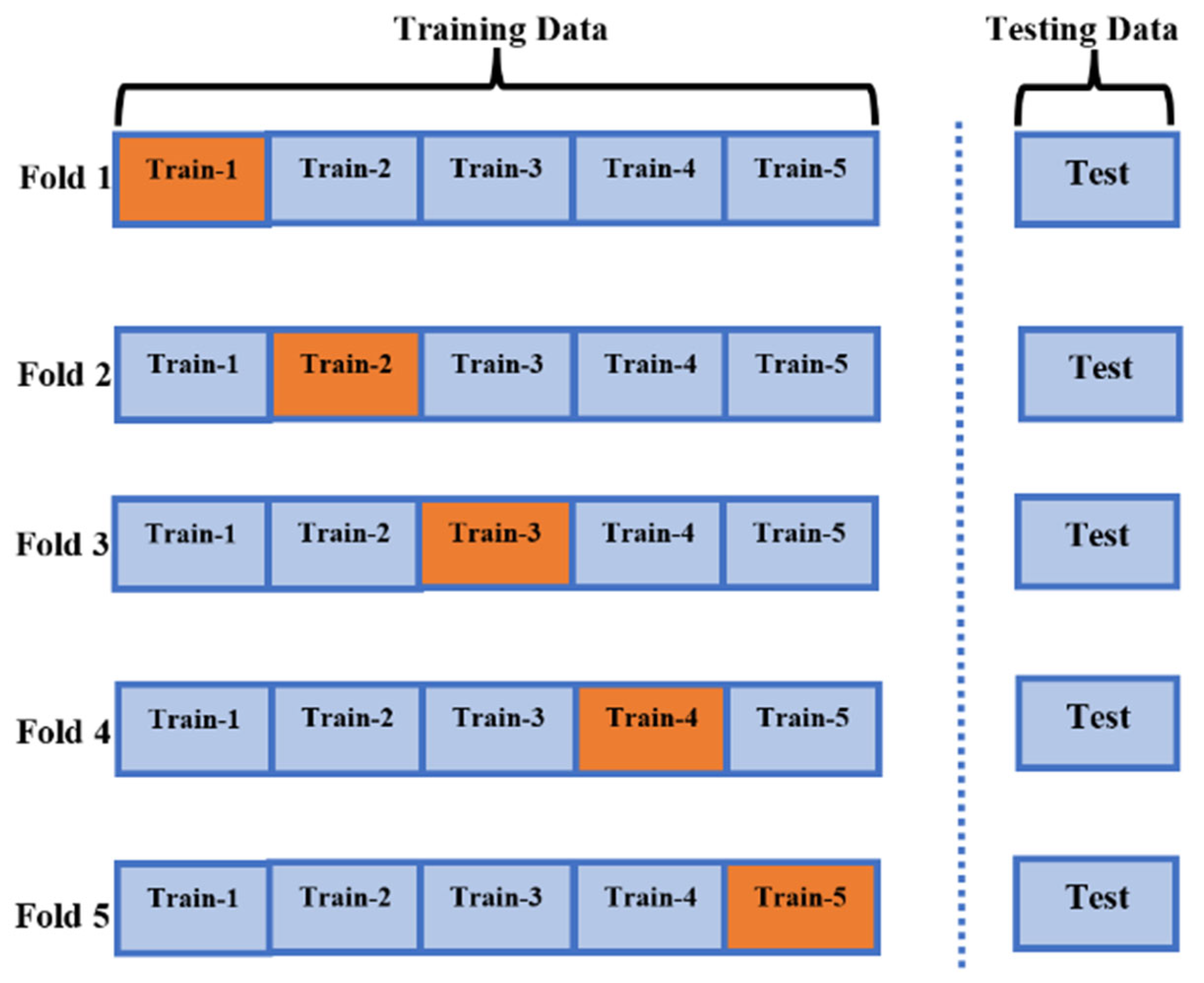
Figure 1. Diagram of the five-fold cross-validation.
Mathematics 10 04361 g001
Figure 2. Crude oil closing price graph.
Mathematics 10 04361 g002
Figure 3. Flowchart of the proposed method.
Mathematics 10 04361 g003
Figure 4. Results for two months with the effect of war.
Mathematics 10 04361 g004
Figure 5. Results for four months without the effect of war.
Mathematics 10 04361 g005
Figure 6. Results for eight months with the effect of COVID-19 for two years.
Mathematics 10 04361 g006
Figure 7. Results for sixteen months with the effect of COVID-19 for one year.
Mathematics 10 04361 g007
Figure 8. Results for thirty-two months without the effect of COVID-19.
Mathematics 10 04361 g008
Figure 9. Graphic of MAE results.
Mathematics 10 04361 g009
Figure 10. Graphic of MSE results.
Mathematics 10 04361 g010
Table 1. LSTM architecture.
Layer NameUsed LayerLayer InputLayer Output
InputInput Layer[(None, 5507, 4)][(None, 5507, 4)]
Lstm_1LSTM[(None, 5507, 4)][(None, 5507, 64)]
Lstm_2LSTM[(None, 5507, 64)][(None, 5507, 128)]
dropoutDropout[(None, 128)][(None, 128)]
dense_1Dense[(None, 128)][(None, 512)]
dense_2Dense[(None, 512)][(None, 42)]
Table 2. Bi-LSTM architecture.
Layer NameUsed LayerLayer InputLayer Output
InputInput Layer[(None, 5507, 4)][(None, 5507, 4)]
Bidirectional_1 (lstm)Bidirectional (LSTM)[(None, 5507, 4)][(None, 5507, 64)]
Bidirectional_2 (lstm)Bidirectional (LSTM)[(None, 5507, 64)][(None, 5507, 128)]
dropoutDropout[(None, 128)][(None, 128)]
dense_1Dense[(None, 128)][(None, 512)]
dense_2Dense[(None, 512)][(None, 42)]
Table 3. Performance results using machine learning.
PeriodPerformance MetricsSVMRFLR
Without ValidationWith ValidationWithout ValidationWith ValidationWithout ValidationWith Validation
Two months (without war)MAE1.64481.65860.78301.41051.13651.1309
MSE3.84513.77041.11202.91011.95361.8942
Four months (low COVID-19 effect)MAE1.59611.57640.88131.51001.19141.1736
MSE4.03893.74841.60334.12572.43282.4214
Eight months (two-year COVID-19 effect)MAE1.09671.08530.56181.00910.85200.8417
MSE2.34402.20220.81162.35951.45971.4528
Sixteen months (one-year COVID-19 effect)MAE0.78690.78500.40480.72340.60960.6033
MSE1.35481.29060.44721.27250.84020.8336
Thirty-two months (without COVID-19)MAE0.92470.92240.37860.70090.50590.5047
MSE7.82727.84401.12295.61410.60170.6340
Table 4. Performance results using deep learning.
PeriodPerformance MetricsLSTMBi-LSTM
2 Months (without war)MAE4.84372.9232
MSE17.954112.9031
4 Months (low COVID-19 effect)MAE8.36906.7242
MSE78.154367.2733
8 Months (two year with COVID-19 effect)MAE9.55677.1789
MSE93.257972.1146
16 Months (one year with COVID-19 effect)MAE7.32836.0759
MSE65.456650.4784
32 Months (without COVID-19)MAE13.62569.9006
MSE160.2515110.8453
Table 5. Performance comparation with the literature.
LiteratureAlgorithmsMAE
Deng et. al. [1]LSTM7.10
Vo et. al. [4]BOP-BL1.2
Busari et. al. [9]AdaBoost-LSTM AdaBoost-GRU1.4164
Yao et. al. [10]LSTM, Prophet2.471
Kaymak et al. [6]SVM15.4211
ANN15.4046
Proposed method (average by months)SVM (without validation)1.160
LR (without validation)0.800
RF (without validation)0.560
SVM (with validation)1.160
LR (with validation)0.790
RF (with validation)1.010
Publisher’s Note: MDPI stays neutral with regard to jurisdictional claims in published maps and institutional affiliations.