Abstract
This article covers a set of models and methods of portfolio investment which help adapt modern economic and mathematical instruments of portfolio investment to the current financial market situation. The main hypotheses serve as a basis for the adaptive dynamic investment portfolio. The experimental analysis shows that the adaptive dynamic investment strategy is more beneficial than classical approaches. The advantage of the adaptive strategy is that it is based on forecast data, whereas classical strategies focus only on historical data.
MSC:
62-08; 91B70; 91B74; 91G10; 91G15
1. Introduction
In reviewing the development of portfolio theory, it should be noted that through different periods it has been altered and elaborated by specialists belonging to various schools and areas of economic and mathematical modeling. However, the terminology used by the adherents of one school is not only insufficient, but even rejected by others.
Each modeling approach has contributed to the development of portfolio theory with its known elements and methods [1,2]. This has led to the appearance of the neoclassical theory of portfolio investment, which is now the basis of all modern systems that model and forecast asset changes under free financial markets.
Table 1 shows the three most prominent directions concerning this sphere of economics, namely, modern portfolio theory, neoclassical theory of investment, and agent-based modeling.

Table 1.
Portfolio investment theories.
Since there are different economic schools and approaches, there are some notions that are not defined properly in portfolio investment theory. To avoid any discrepancy, the following notions are used in developing the adaptive portfolio model:
- Investment is a process of allocating funds in assets in order to make profit.
- Investment strategy is an investor’s decisions that are determined by rules and restrictions that create boundaries for investment represented by profitability and risk.
- Market stability means that there is a balance of supply and demand most of the time;
- Market predictability means that the market is predictable most of the time;
- Preference for forecast means that the forecast is more preferable than its absence;
- Crises inevitability means that there are phase changes in any open and evolving system.
As it follows from the aforementioned axioms, the main hypotheses are as follows:
- Advantages of the adaptive strategy: a change in the investment strategy (adaptation to changes in portfolio-market system) is more preferable than suffering losses;
- Advantages of the dynamic portfolio: an investment portfolio with a dynamic strategy is more preferable than a portfolio with a fixed strategy.
We review the classical papers devoted to the topic of our study.
Statman in [3] uses a portfolio formed from a list of 500 selected US joint-stock companies. He empirically justifies that a well-diversified portfolio must include at least 30 stocks for a borrowing investor. This contradicts the classic statement that if a portfolio contains approximately 10 stocks, then the benefits of diversification are virtually exhausted. In his study, Statman refers to the fact that diversification brings not only benefits but also costs; therefore, it must be increased until the marginal benefit exceeds the marginal cost.
Chen [4] suggests applying a tree-like set of IF–THEN statements with confidence rules on a tree-like population of hypothetical portfolios corresponding to a set of possible market states to optimize a portfolio strategy.
Authors Nikolakakis and others [5] suggest building investment strategies based on government plans for the power sector development. As a justification, they provide an empirical explanation that where there is an excess of energy, the economy begins to grow rapidly in all areas.
In the work of Francesco P. Appio et al. [6], based on the case study of the patent market, two elements of the strategy are compared as antagonistic indicators: diversification and monopolization of the portfolio. Based on empirical data on the asset allocation in real patent portfolios, the authors found that the relationship of these indicators to risk is nonlinear. The risk of a partially diversified portfolio is usually two or more times higher than that of a fully monopolized or fully diversified portfolio.
The authors Rupert Way, Francois Lafond, Fabrizio Lillo, Valentyn Panchenko, and J. Doyne Farmer [7] propose to determine the necessary degree of portfolio diversification by evaluating the progress rate of assets, the variability, and the initial cost of the portfolio. They offer a dynamic model with a gradual change in diversification, increasing as asset quality deteriorates.
In the work of Jacques Pezier and Joanna Scheller [8], the authors compared two portfolio models applied to equal pension payments. The authors showed that more frequent, but smaller, payments make a portfolio more investment-attractive than larger, less rare payments.
Authors Vo, Nhi NY, Xuezhong He, Shaowu Liu, and Guandong Xu [9] suggest abandoning both classical and modern portfolio theories and entrusting investment portfolio management to a multilayer neural network with deep learning. When operating on theoretical data, such a network shows very impressive results; however, as the authors themselves note, during the initial period of practical training of the network, investors will suffer significant losses.
Authors Yasemin Deniz Akarim and Serafettin Sevim [10] conducted an empirical study using panel analysis to compare near-static portfolios containing stable, well-growing assets with portfolios used for constant trading emerging-market assets. The authors show that with a well-chosen strategy, consistently developing near-static models are superior to models with emerging-market assets, despite trading and arbitrage.
Authors Gaurav Jadhao and Abhijeet Chandra [11] suggest using the sample entropy indicator and the volatility index to determine the moment of portfolio rebalancing. The authors, using the above indicators, empirically tested 130 different portfolio strategies and found that the entropy indicator performs significantly better than aggregate indices such as MSCI.
The authors Jiaqin Wei, Yang Shen, and Qian Zhao [12] propose the simplest two-regime dynamic portfolio model that has a relative risk aversion regime and absolute risk aversion regime and switches the strategy depending on arbitrarily determined external risk factors.
The authors Ma G., Siu C. C., and Zhu S. P. [13] propose a dynamic portfolio that is optimized based on the analysis of the predicted market situation, instead of relying on the current trends. In fact, the authors recommend using the classic Merton portfolio, optimized based on the expected market conditions.
The authors Zhilin Kang, Linhai Zhao, and Jingyun Sun [14] suggest using a static VaR-optimal portfolio model. In fact, the authors suggest adding high-risk assets to the portfolio until the VaR reaches a preplanned maximum.
The authors Zhifeng Dai and Fei Wang [15] argue that the losses in portfolio investment are caused by insufficient information about assets and the market, that is, by estimation errors in input parameters of the portfolio model. The authors propose a mathematical portfolio optimization model that is aimed not so much at increasing the portfolio return, but rather at ensuring robustness to incomplete information.
The authors Lu Y. N. et al. [16] suggest splitting the investment portfolio into several different portfolios with different strategies. In this way, the method of strategic diversification is implemented. In fact, in this paper, the authors describe a new method of portfolio diversification, namely, strategic diversification.
The author Young Cheol Jung [17] suggests insuring the portfolio against an increase in the volatility index. The author argues that when the market becomes volatile, it is possible and necessary to use insurance against volatility.
The authors Lin Ling, Zhou Zhongbao, Liu Qing, and Jiang Yong [18] consider the empirical effect of risk transmission from real sectors of the economy to stock markets. Arguing that technical analysis is not sufficient for portfolio investment, the authors suggest monitoring not only financial markets but also microeconomic indicators.
The work of Liu Y. J. and Zhang W. G. [19] is dedicated to practical issues of determining the optimal time horizon of investment and portfolio tracking periods. The authors, based on experimental data, conclude that the depth of the time horizon inversely depends on the expected frequency of trading.
The authors Chen J. S. et al. [20] suggest using a genetic algorithm to optimize a portfolio for a given level of risk or return. Empirically, as the authors show, in a number of experiments, the effect of using the genetic algorithm exceeds the naive diversification.
The analysis of time series is described in the works of the following authors.
The authors Kunitomo et al. [21] investigate the estimation methods of the multivariate nonstationary errors–invariables models when there are nonstationary trends. The authors Banerjee et al. [22] consider the econometric analysis of both stationary and nonstationary processes.
The authors Pesaran et al. [23] develop a new approach to the problem of testing the existence of a level relationship between a dependent variable and a set of regressors.
Johansen [24] gives a mathematical and statistical analysis of the cointegrated vector autoregressive model.
The article [25] talks about the benefits and advantages of the mean absolute error (MAE) over the root mean square error (RMSE) in assessing average model performance.
2. Practical Implementation of the Simulation Model of a Dynamic Investment Portfolio
Description of an adaptive investment strategy simulation model for a dynamic portfolio.
The aim of the study was to build an adaptive investment strategy that minimizes losses in the financial market and to compare the developed investment strategy with classical strategies. The criterion for comparison was the indicator of efficiency and profitability of the portfolio.
The developed model allows to reduce losses or reduce them to zero. The usefulness of the model lies in its resistance to crisis processes in the financial market.
The scientific significance of this study lies in the fact that the neoclassical portfolio solves the problems associated with outdated investment strategies.
In addition, special attention was paid to the implementation of the algorithm for building an investment portfolio (Figure 1) in which an important role is given to forecasting models and risk assessment.
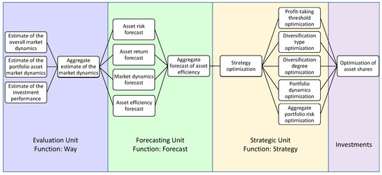
Figure 1.
Algorithmic flowchart of an adaptive investment portfolio.
Figure 1 shows an algorithmic flowchart of an adaptive investment portfolio. The algorithm consists of the following units:
- Section 2.1 Evaluation Unit. Analytical indicator of the market state
- Section 2.2 Forecasting Unit. Ensemble Asset Value Forecast.
- Section 2.2.1 Aggregate Forecast of the Total Asset Risk.
- Section 2.3 Strategic Unit.
- Section 2.4 Investments. Optimization of asset shares.
Let us assume that strategic investment, which is understood as a minimum existence period of the strategic portfolio, is 7 years. For a preliminary assessment, it is necessary to have a minimum prior period of 1 year. Thus, the minimum time for creating a mathematical model of a strategic investment portfolio is 8 years. Based on empirical data and conclusions presented in the work of Makridakis and Taleb [26], taking the statement about the low degree of predictability of market processes, we shall determine the maximum predictive and analytical period of the model [1,2].
To achieve this, we will be guided by the sufficiency rule of the information completeness described and proved by Kotelnikov and Shannon [27,28]. According to the general conclusion from this work, the information completeness of the signal description is achievable only if the frequency of the level measurements is twice as high as the frequency of the signal change or exceeds this threshold value. In other words, considering changes in the value of an asset as a conditionally continuous signal, it is possible to determine the maximum allowable duration of the required observation period as , where f is a value proportional to the required level of statistical significance.
Based on the above and the average duration of the investment year d, which is equal to an average of 247 trading days, let us determine a sufficient degree of rounding of the time scale with a statistical significance of at least .
According to the theorem of Kotelnikov and Shannon [27,28], in order to maintain accuracy, the scale interval must correspond to .
Using the typical value of 0.01, which is the nearest to , we obtain the value of the minimum period of the portfolio observation , as shown in Equations (1) and (2):
where is the analytical period (observation interval), Y is the investment period in years, d is the duration of the investment year in days, and is the required statistical significance.
With strategic investment, for statistical significance , , :
Thus, the analytical period required for strategic investment corresponds to 20 days.
Next, the following notation is used in the work: —the observation period is 1976 days; T—the investment period is 1729 days; —the analytical period is 20 days; —the minimum scale interval is 1 day; t—the period from the beginning of the observation, expressed in .
Then, everywhere, t is accepted as an argument.
To implement the mathematical model, it is necessary to define a unified system of scales, as well as to determine the main intervals of values for each parameter of the model, resented in Table 2.

Table 2.
Mathematical model scale system.
The normalization interval is calculated based on the following Equations (3)–(5). Normalization of positive value:
Normalization of the sign value:
Reduction of the sign value:
Table 3 describes the normalized scale of market states and portfolio states .

Table 3.
Normalized scale of market states and portfolio states.
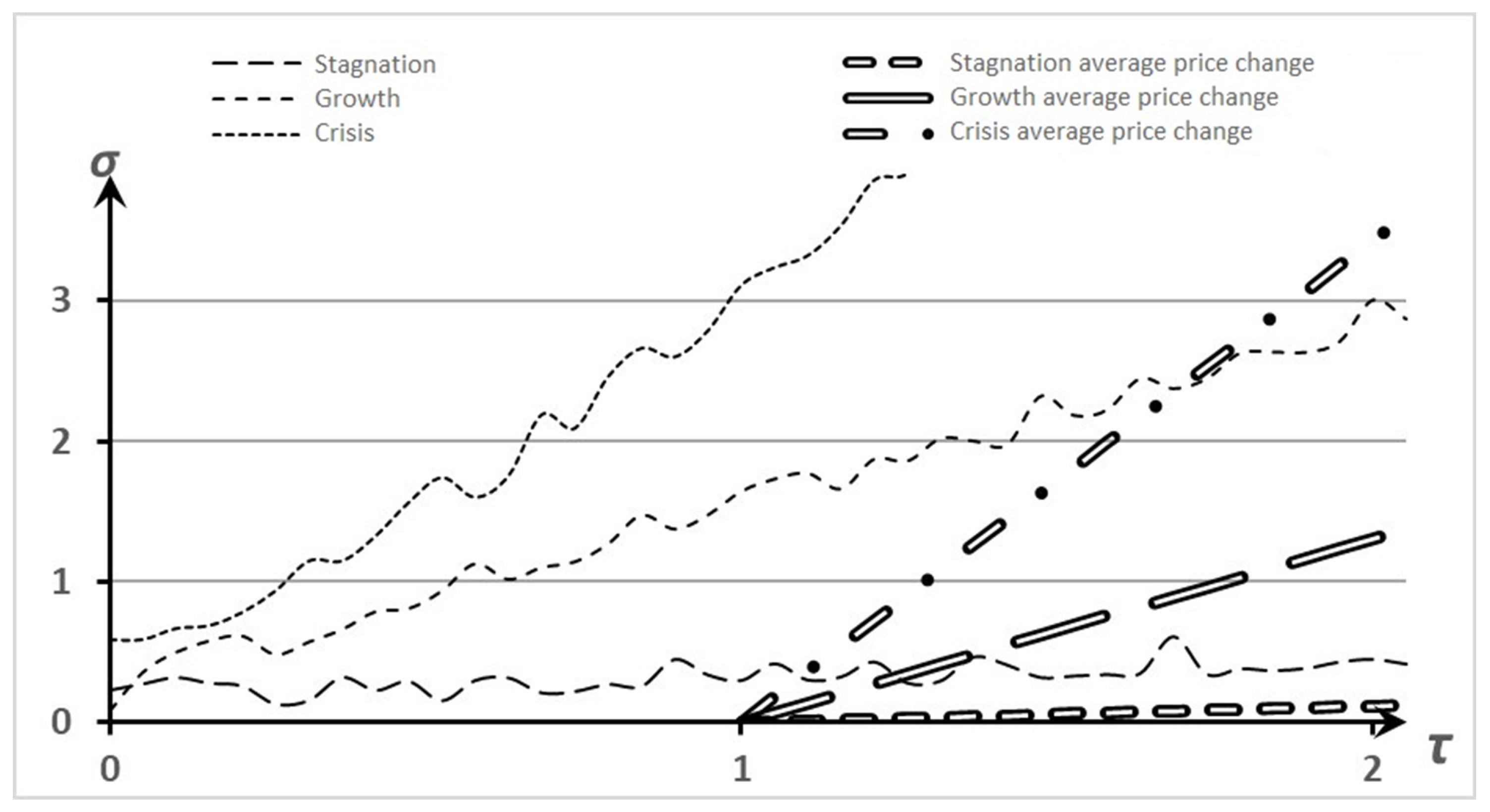
For further ranking, we take as the boundaries of the asset price fluctuations its standard deviation, presented in Table 4 and Figure 2.

Table 4.
Scale of return boundaries.
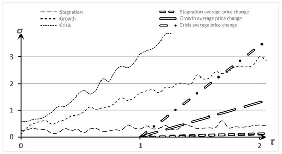
Figure 2.
Ratio of asset price change to standard deviation.
Next, we consider the implementation of this algorithm on practical data.
2.1. Evaluation Unit. Analytical Indicator of the Market State
The mathematical expression for the analytical indicator is according to Formula (6).
where —an indicator of the reduced return on the asset, , H—Heaviside function; —Kronecker function; —the absolute return of the i-th asset in the period ; —the maximum return of the i-th asset in , achieved over the entire historical period; —standard deviation of the price of the i-th asset in the period ; —accumulated standard deviation of the i-th asset.
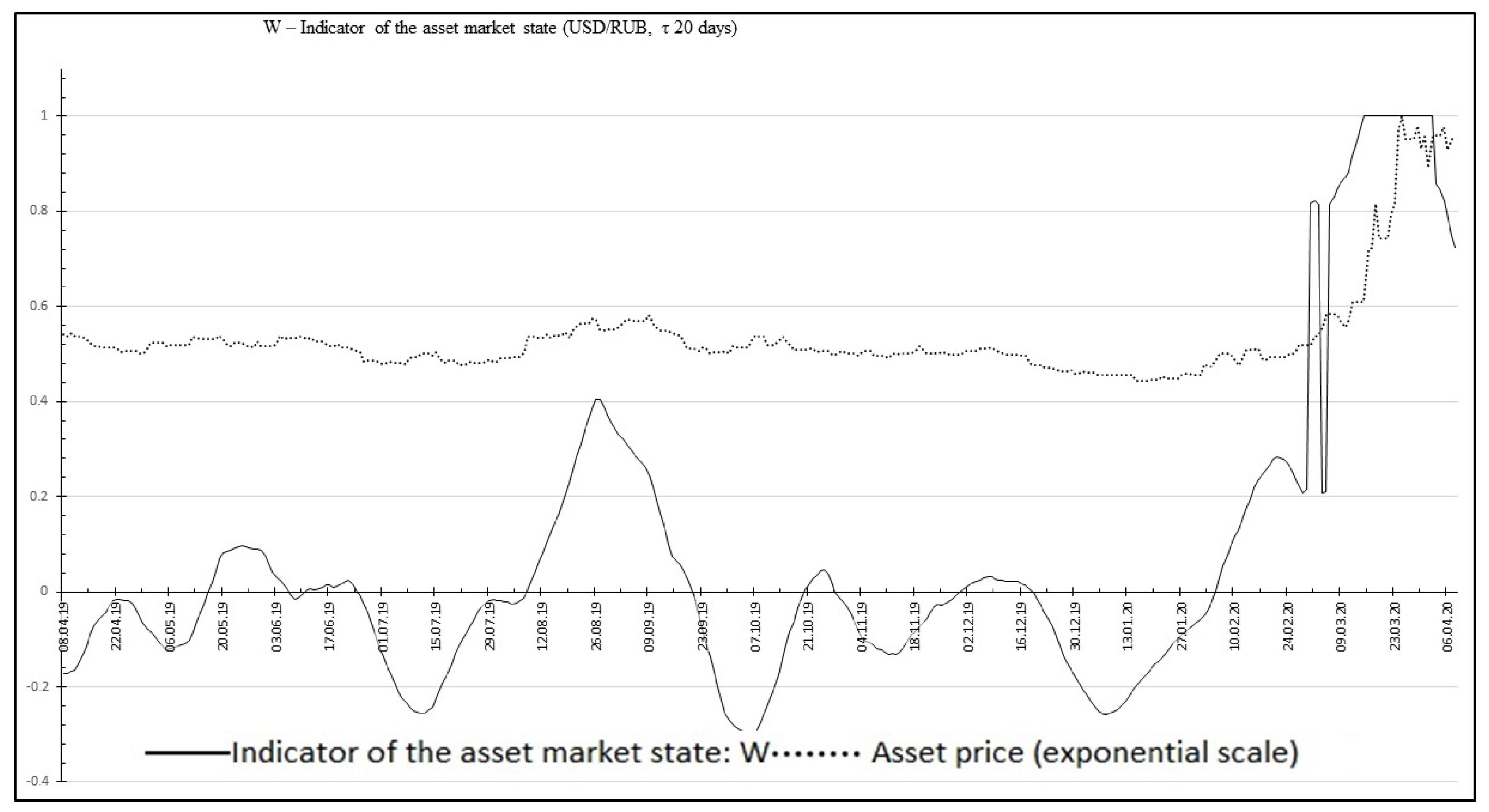
The result of using the function is shown in Figure 3.
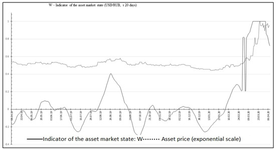
Figure 3.
Graph of applying the function to historical asset price data.
The mathematical expression for the reduced analytical indicator is as shown in Formula (7).
where —the portfolio indicator of the reduced return; —the indicator of the reduced return of the i-th asset; —the share of the i-th asset in the portfolio; n—the number of assets in the portfolio.
2.2. Forecasting Unit. Ensemble Asset Value Forecast
The mathematical expression for the multitrend forecast of the asset value is as shown in Formula (8).
where —the multitrend forecast of the asset value; —the linear forecast of the asset value; —the asymptotic linear forecast of the asset value; —the indicative forecast of the asset value; —the asymptotic indicative forecast of the asset value; —confidence coefficients of the corresponding forecasting methods.
The result of the multitrend forecast is shown in Figure 4.
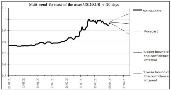
Figure 4.
The result of the multitrend forecast for 20 days ahead for the USD/RUB asset.
Method: Wavelet asset value forecast :
where —the value of the i-th wavelet at time t; a—the wavelet amplitude; b—the wavelet compression coefficient; c—the wavelet decay coefficient; d—the wavelet shift coefficient; t—time.
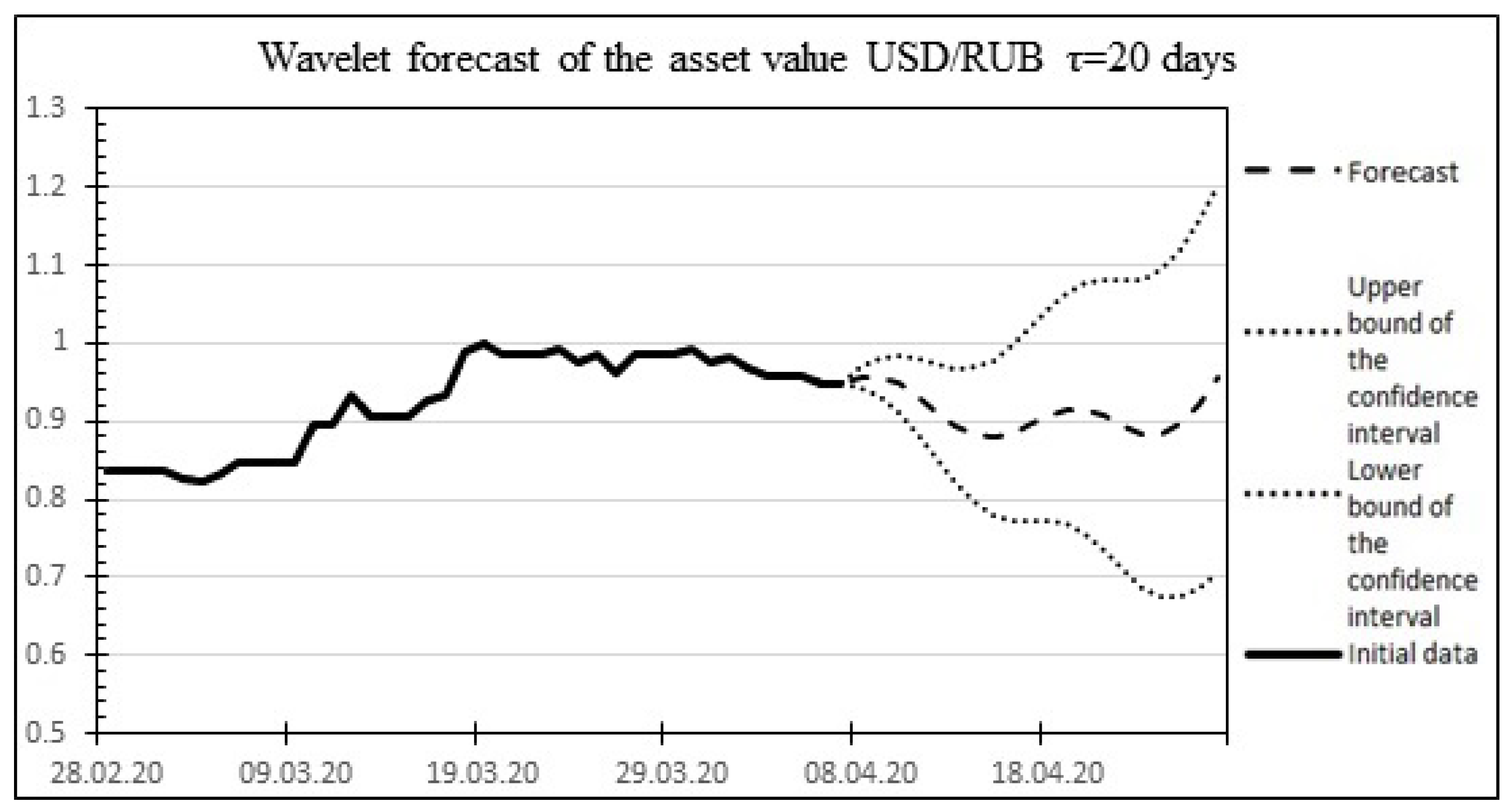
The result of the wavelet forecast is shown in Figure 5.
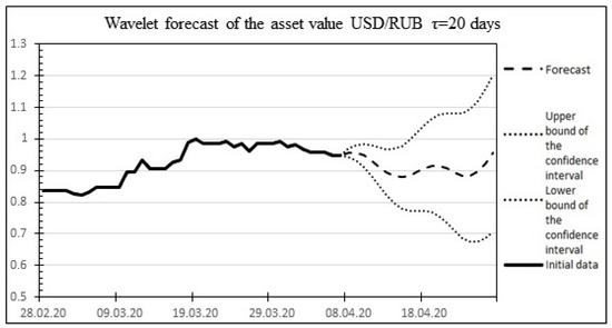
Figure 5.
The result of the wavelet forecast for 20 days ahead for the USD/RUB asset.
Method: Neural asset value forecast :
where —the price forecast by the recurrent network at time t; —the depth of historical data for the forecast; —the asset price at time t; —the Verhulst function; m—the number of input neurons; n—the number of inputs of each neuron of the first layer; i—neuron number; j—the number of the neural network input; —coefficients of the input weights of the neuron calculated during training; —neuron recursion coefficients calculated during training.
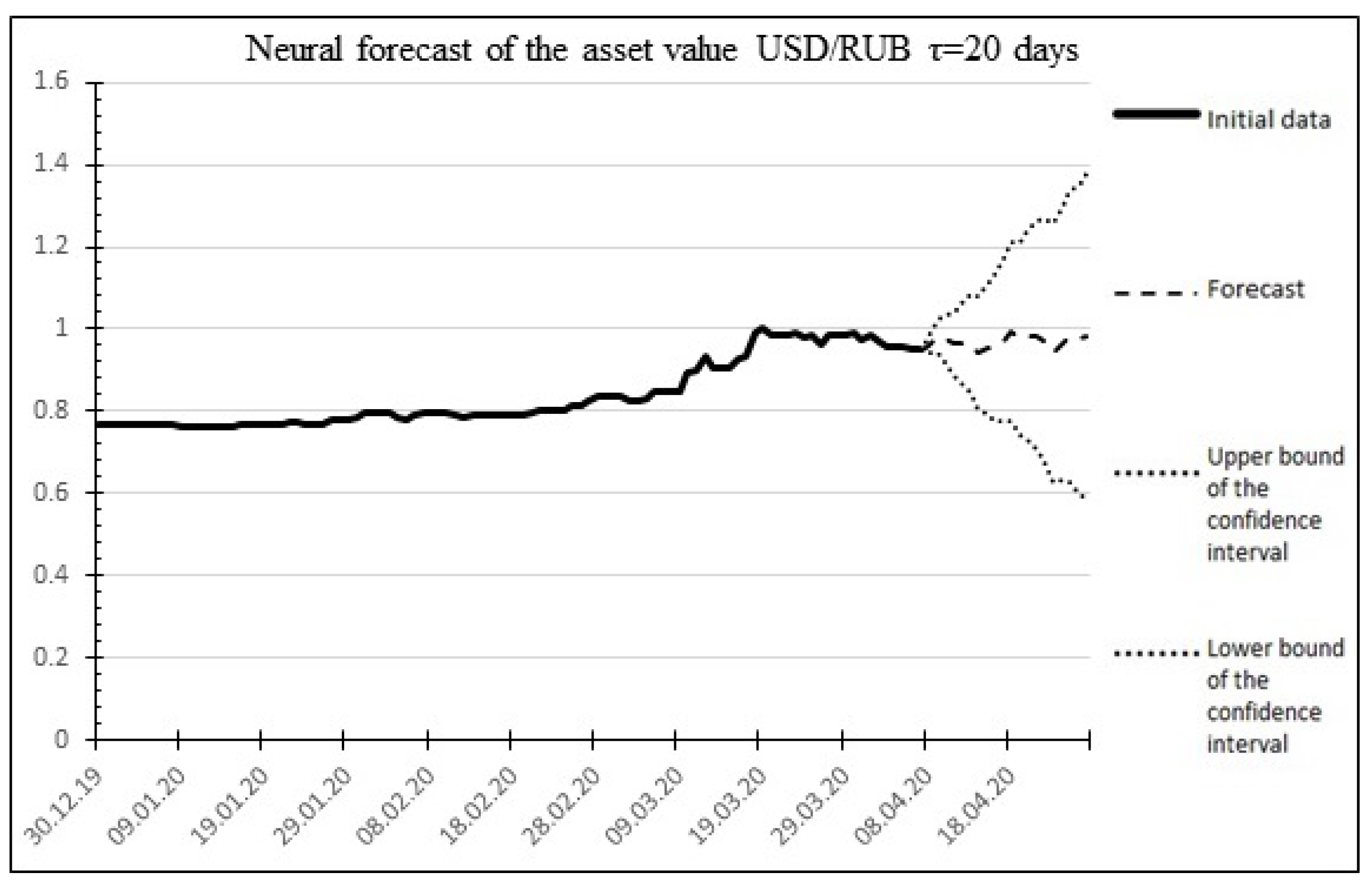
The result of the neural forecast is shown in Figure 6.
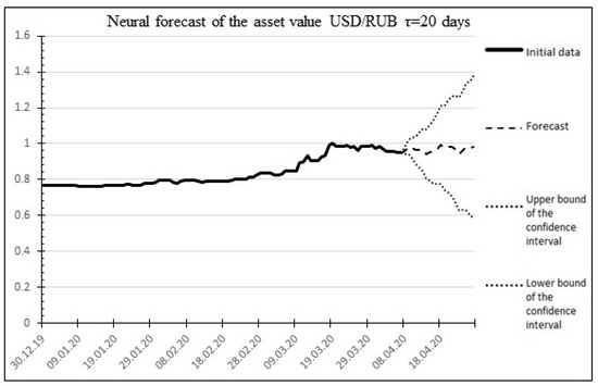
Figure 6.
The result of the neural forecast for 20 days ahead for the USD/RUB asset.
Method: The aggregate ensemble forecast of the asset value :
where —the aggregate forecast; —the multitrend forecast; —the neural forecast; —the wavelet forecast; —corresponding confidence coefficients.
where —corresponding confidence coefficients; —confidence intervals of the corresponding methods.
Confidence interval of the forecast:
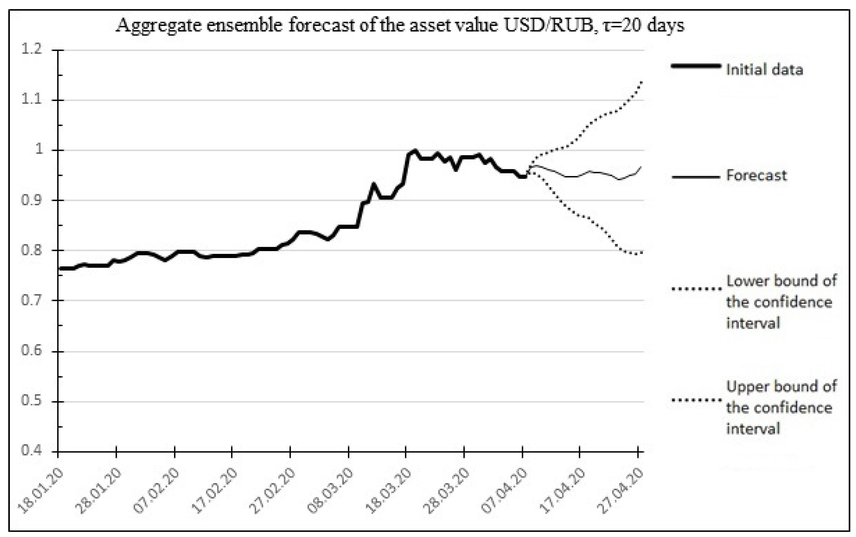
The result of the aggregate forecast is shown in Figure 7.
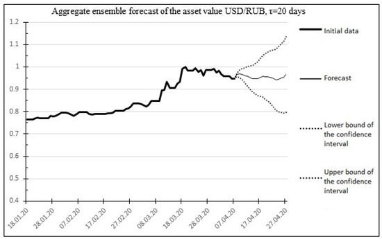
Figure 7.
The result of the aggregate forecast for 20 days ahead for the USD/RUB asset.
However great the variety of forecasting methods may be, they can be divided into two ideologically opposite groups. Thus, the first group includes idealized forecasting methods based on mathematical models that assume universal quasistationarity as a manifestation of ergodicity. The second group includes forecasting methods that are more generally applicable because they consider the concept of ergodicity as a statistical phenomenon and deny the existence of both global and local stationarity.
By introducing the notion of the limitation of existence, these methods assume only the presence of certain tendencies while denying their quasistationarity. This is the difference between portfolio theory of G. Markowitz and Neoclassical Portfolio Theory. G. Markowitz’s theory assumes the infinite stationarity of financial and exchange trends and is built on the idealized model of "Buy and Hold". The neoclassical theory, considering these trends not stationary, requires continuous observation and appropriate rebalancing.
From the author’s point of view, confirmed by repeated local and global financial crises, it is categorically wrong to consider the market as a stationary system. One can only observe the existing trends and rebalance the portfolio by assessing these trends at the moment. This point of view is represented in the dynamic portfolio method which involves continuous observation of trends and appropriate rebalancing. Thus, without being able to build a stationary model of the change in the price of an asset, we can rely solely on statistical prediction methods based on short-term data that have the ability to become obsolete, according to Makridakis [26]. Thus, the assessment of the quality of forecasting can be carried out exclusively de facto using descriptive point estimates as its main characteristics. The quality estimation of a forecast will be its standard relative error (RMSE).
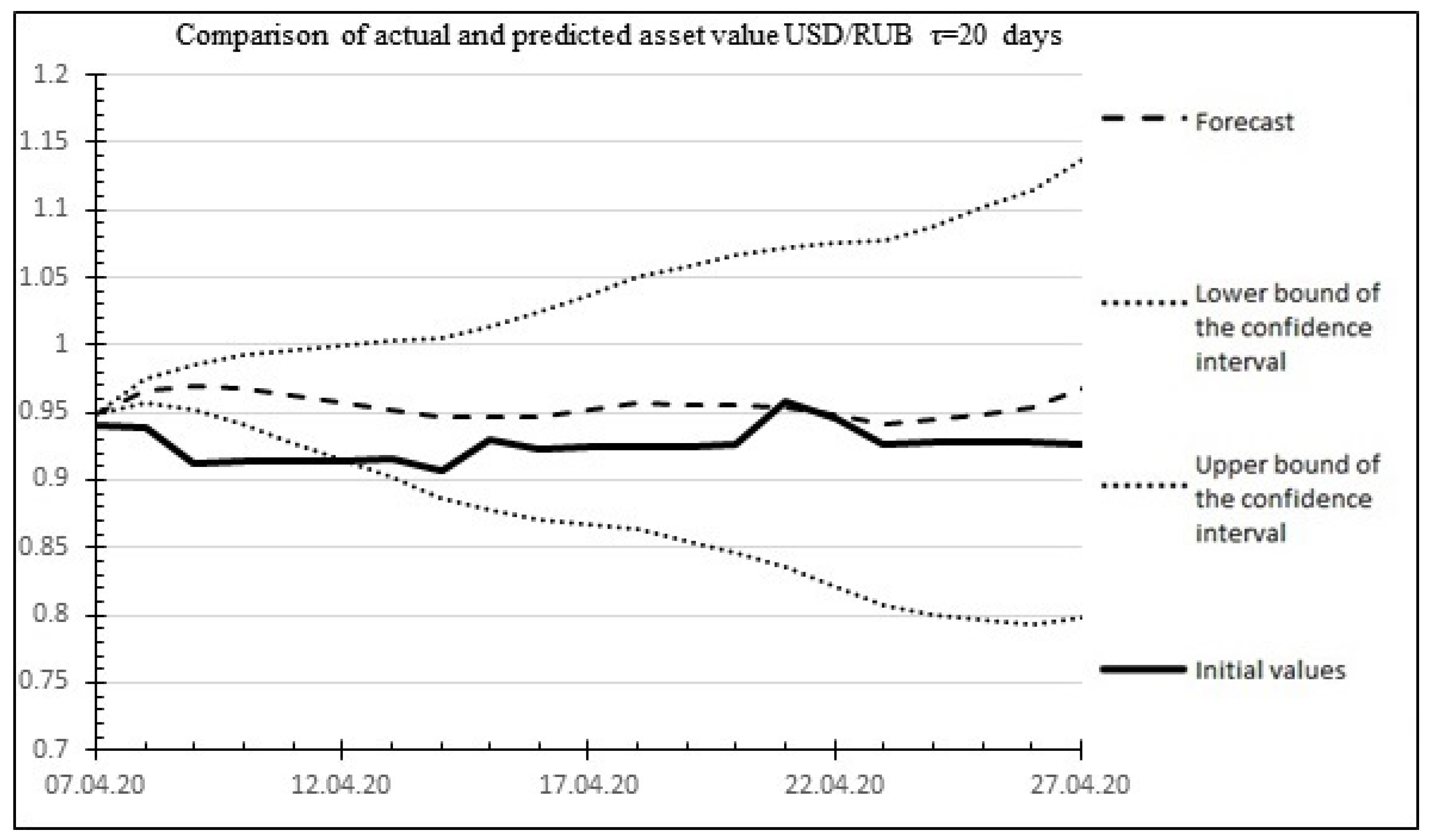
Figure 8 shows a graph comparing the predicted and actual values of the asset value.
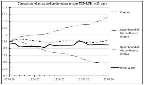
Figure 8.
Comparison of the results of the 20 days ahead forecast of the USD/RUB asset value with actual values.
Percentage error: 4.3962%.
2.2.1. Aggregate Forecast of the Total Asset Risk
The aggregate forecast of systematic risk is formed in the same way as the abovementioned forecast of return, with the difference that the initial data are the values of the current systematic risk determined for the analytical period: the standard deviation of the price for the last 20 days. Below shows the practical results and statistics of forecasting systematic risk for the USD/RUB asset and the components of the aggregate forecast.
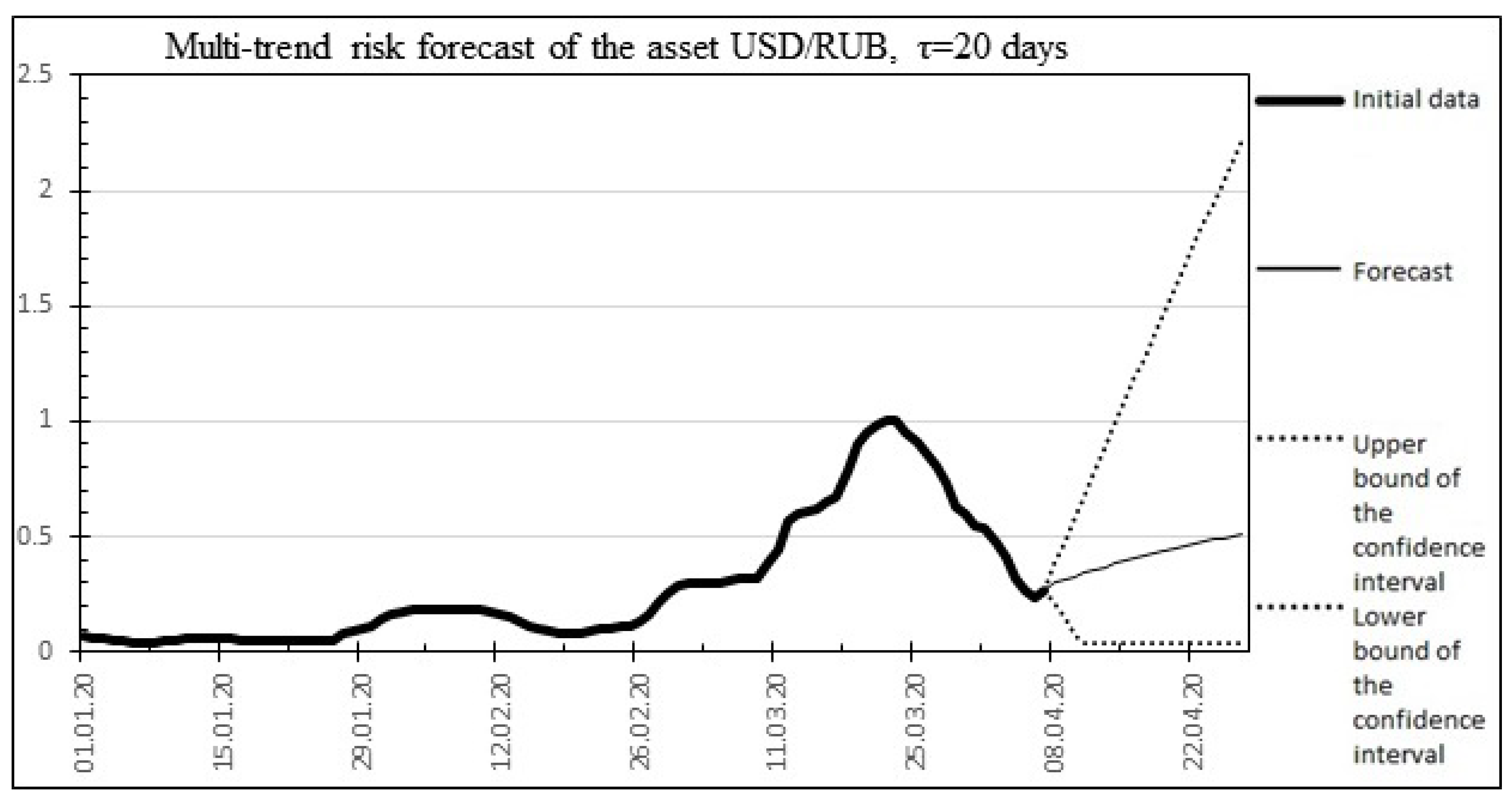
Method: Multi-trend asset risk forecast :
The result of the multi-trend risk forecast is shown in Figure 9.

Figure 9.
Multitrend risk forecast.
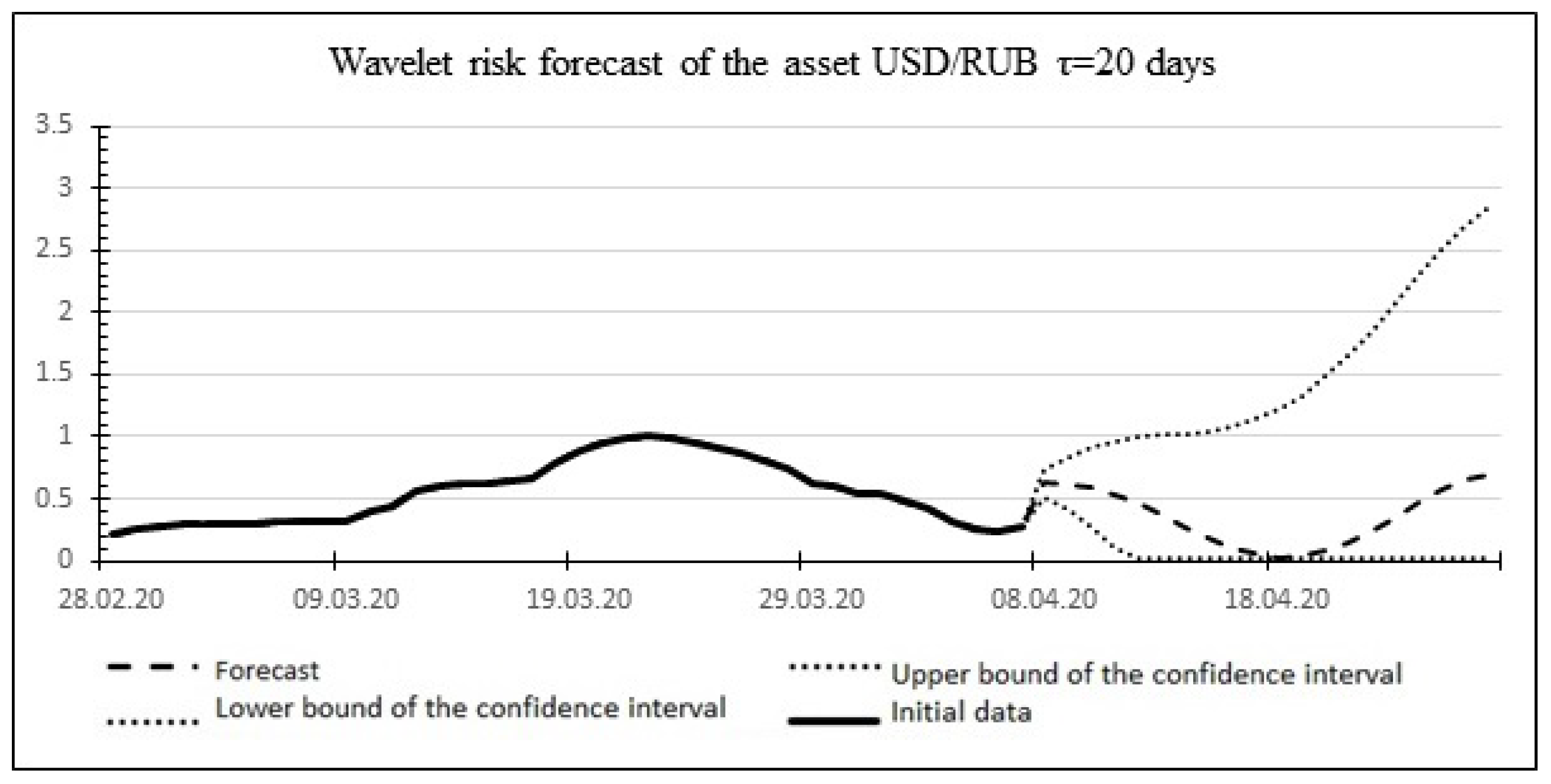
Method: Wavelet asset risk forecast :
The result of the wavelet forecast is shown in Figure 10.
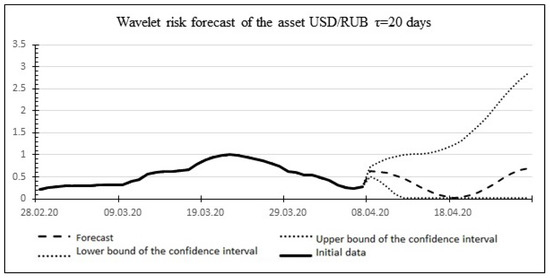
Figure 10.
Wavelet asset risk forecast.
Method: Neural asset risk forecast:
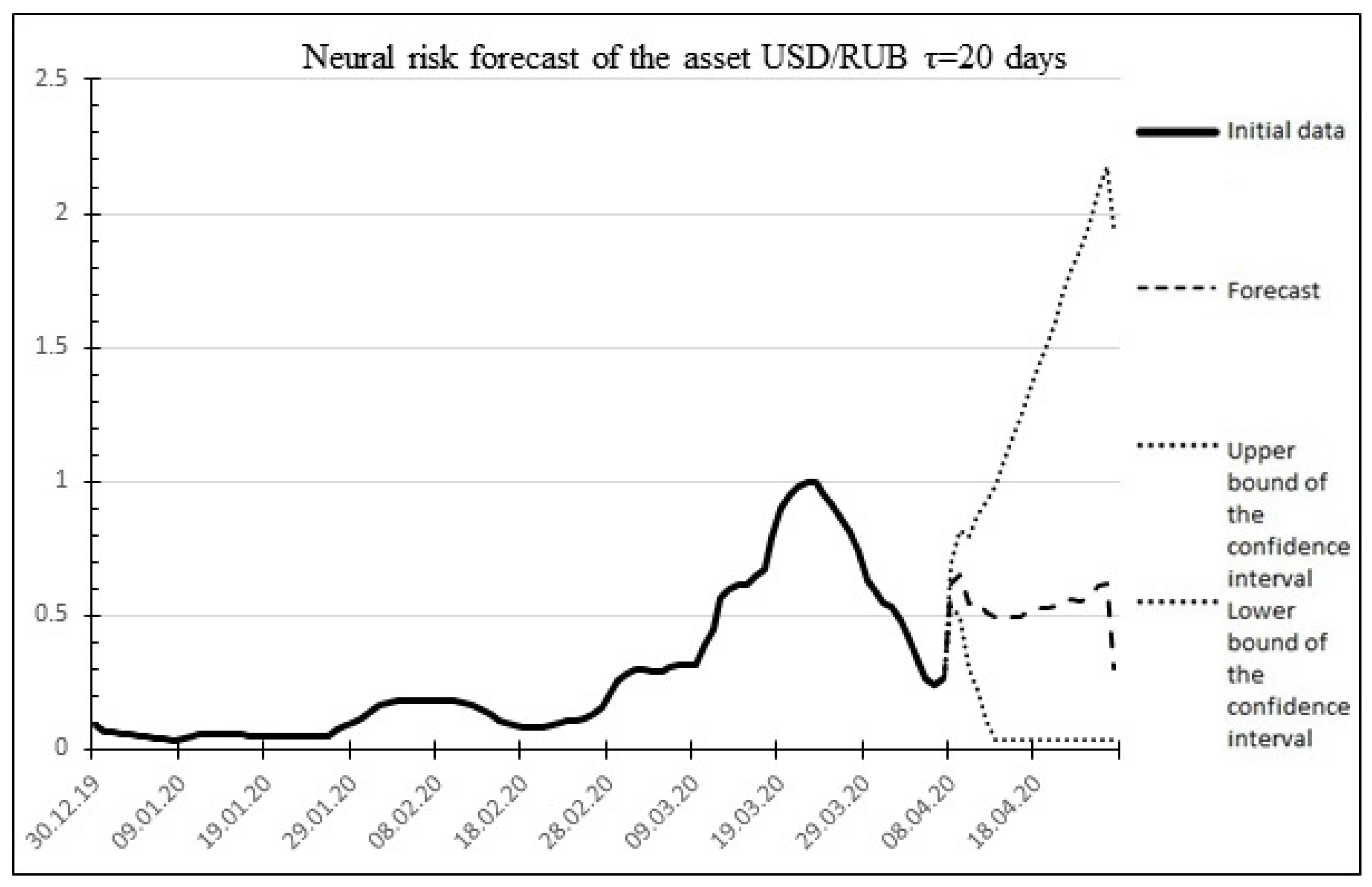
The result of the neural forecast is shown in Figure 11.
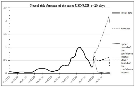
Figure 11.
Neural asset risk forecast.
Method: The aggregate forecast of the systematic risk of the asset .
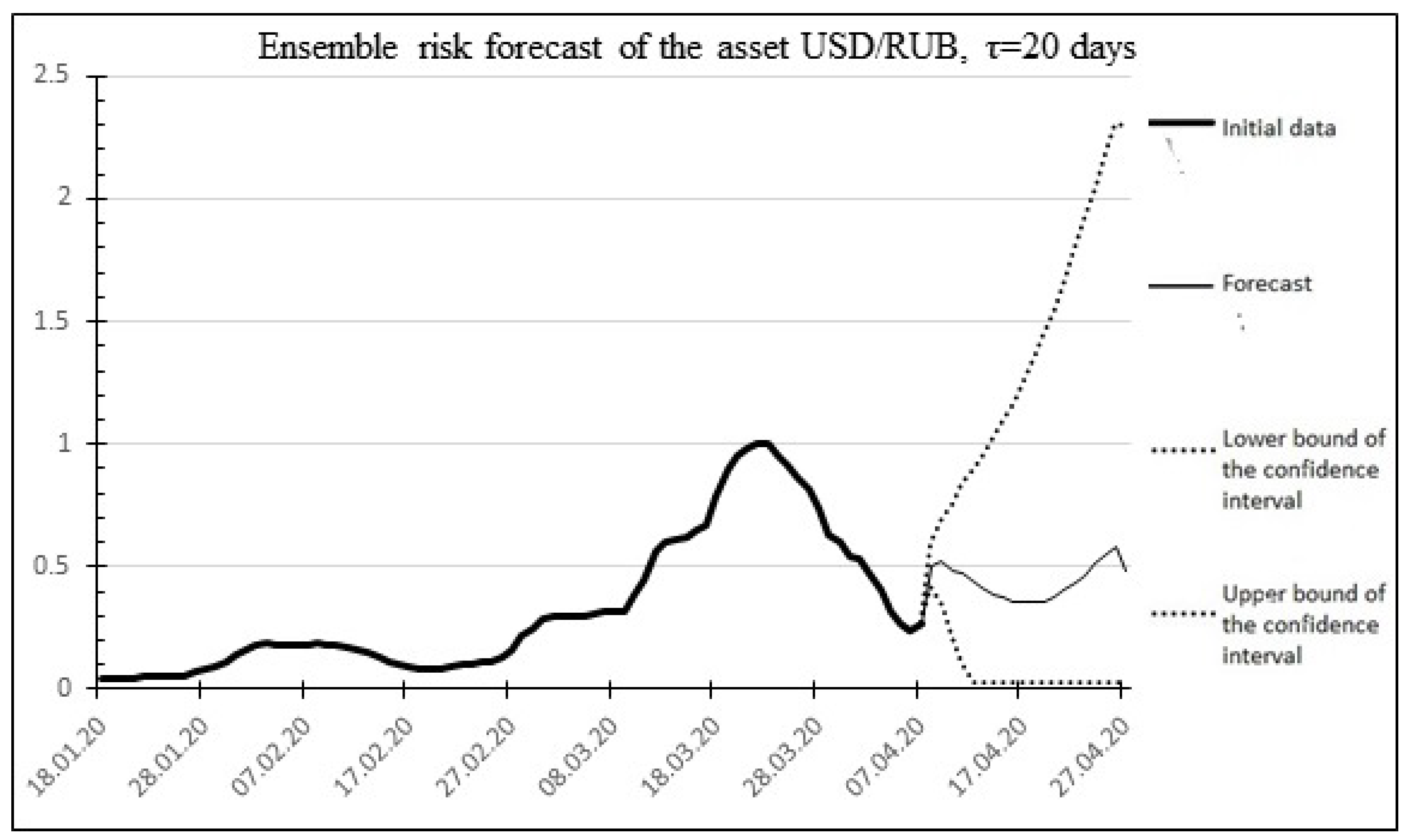
The result of the ensemble (aggregate) forecast is shown in Figure 12.
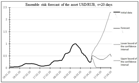
Figure 12.
Aggregate ensemble risk forecast for the USD/RUB asset.
Percentage error: 7.405701%.
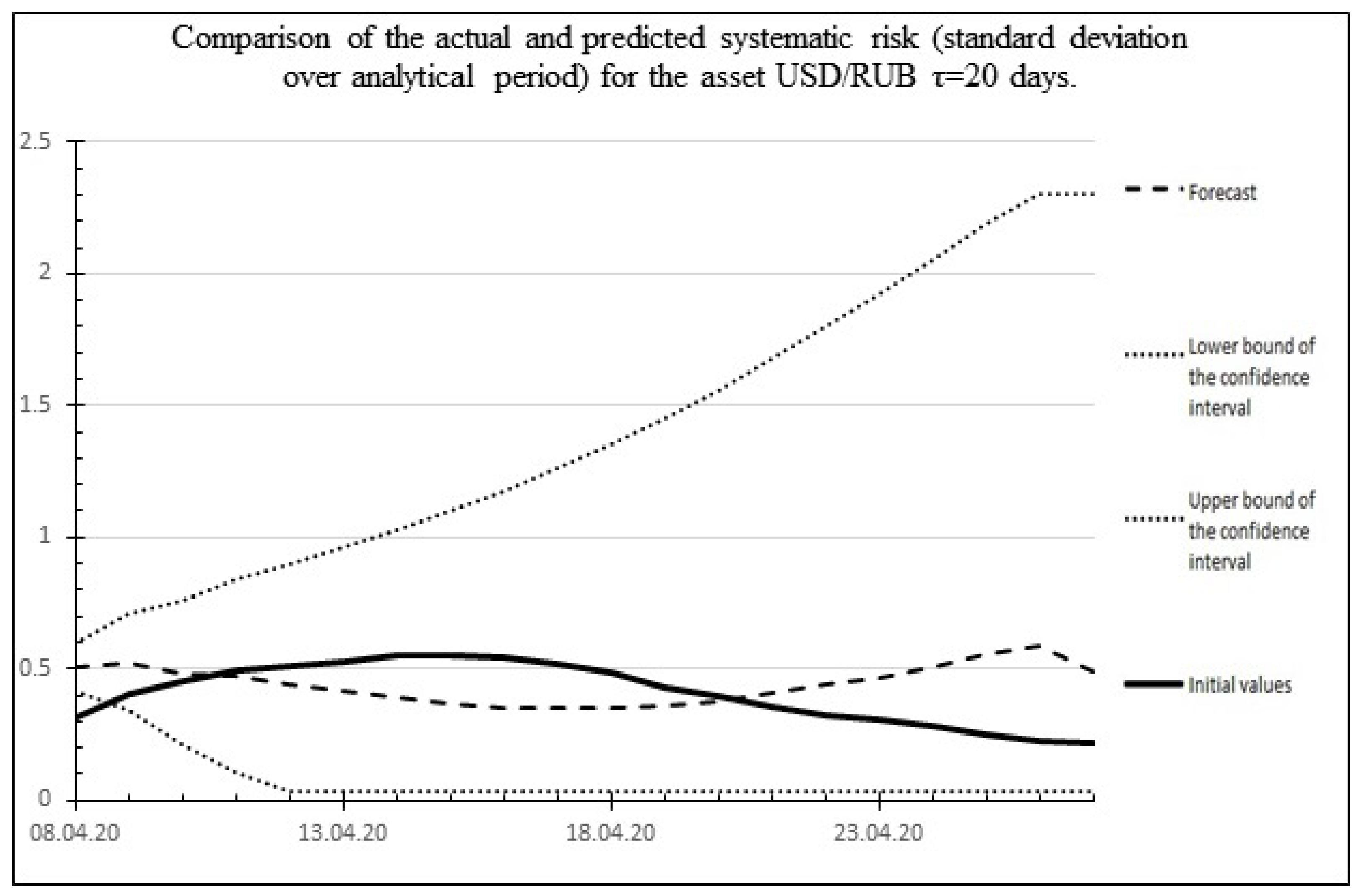
Figure 13 shows a comparison of the actual and predicted systematic risk for the USD/RUB asset.
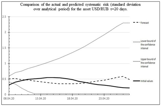
Figure 13.
Comparison of the results of the 20 days ahead forecast of systematic risk of the USD/RUB asset with actual values.
The aggregate forecast of the total asset risk is . The risk of unconditional rebalancing losses is .
where —the risk of unconditional rebalancing losses (loss risk); —the number of rebalancing events actually performed during the period t; —the duration of the analytical period; t—the time period defined in the minimum intervals of the time scale; —the minimum time scale interval.
For example, for the USD/RUB asset, the risk of unconditional rebalancing losses calculated on 29 February 2020 is equal to 0.074237 [29].
Risk of a crisis change in the asset value:
where C—the indication of the presence of an asset crisis; —the noncrisis standard deviation for ; —the largest standard deviation during the period of the i-th crisis; —the time elapsed since the beginning of the asset crisis; —the average duration of crises of the selected asset; k—the number of past asset crises; —Holt’s data deterioration coefficient.
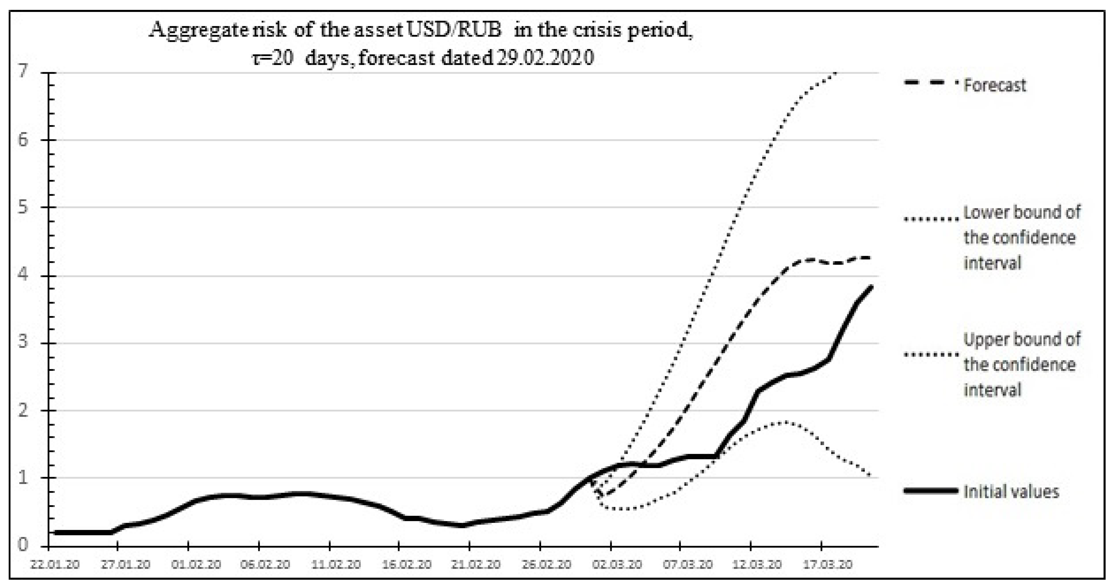
Below, as an example, Figure 14 shows the risk forecast and actual values for the USD/RUB asset for the time of the global economic crisis of 2020, which occurred in the period from 29 February 2020 to 2 April 2020. The historical values of the duration of the crises and the increase in standard deviations obtained based on historical data on the US dollar exchange rate published on the website of the Central Bank of the Russian Federation (Table 5) are used as the initial data for the calculations:
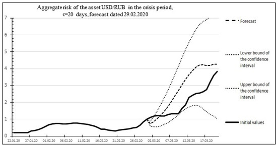
Figure 14.
Final statistics of the initial data and results of the USD/RUB asset risk forecast during the crisis period.

Table 5.
Initial data for calculating the crisis risk.
Aggregate forecast of the total asset risk
The mathematical expression is as shown in Formula (20):
Figure 14 shows an example of the aggregate risk of the USD/RUB asset and the statistics of the forecast and actual risk values for the USD/RUB asset. Percentage error: 6.79459%.
2.3. Strategic Unit
The projected return on the asset:
where —predicted profitability of the i-th asset in the portfolio for the period ; —confidence coefficients; V—the value of the portfolio.
Projected increment in the asset risk:
Projected efficiency of the portfolio asset:
Profit-taking threshold:
Type of portfolio diversification:
Degree of portfolio diversification:
where —the estimate of the current state of the portfolio asset market; —the recommended coefficient of portfolio diversification.
Degree of portfolio dynamism:
Actual aggregate portfolio risk:
Analytical indicator S:
Projected portfolio efficiency:
where —the projected efficiency of the portfolio over the period ; —the portfolio share of the asset; —the projected return on the asset over the period ; —the projected aggregate risk of the asset over the period ; n—the number of assets in the portfolio.
2.4. Investments. Optimization of Asset Shares
By presenting the projected portfolio performance as a geometric measure of the differences in the projected return and risk of assets, it is possible to maximize its estimated future value by calculating the weights of the portfolio shares of assets, taking into account the portfolio bounds determined by the strategy, which in turn is determined by the state of the market of portfolio assets, as shown in the following formula:
3. Comparative Analysis of the Portfolio Model Quality
Let us develop objective evaluation criteria and conduct an analysis to obtain a performance comparison of classical models with an alternative (adaptive investment model being developed).
The following basic criteria of evaluation were introduced:
- The level of abstraction (A—the reciprocal of the number of basic variables N).
- The test of the mathematical complexity evaluation , where M—the number of strategy elements.
- The test of the practical implementation complexity evaluation , where H—required man-hours, P—required machine-hours.
- The base complexity level (a measure of complexity), represented by the complexity of H. Markowitz’s model.
- Overall rating (the reciprocal of the product of mathematical and practical complexity by the value of abstraction ). The model comparison yielded the results shown in Table 6.
 Table 6. Evaluation criteria of investment portfolio models and objective assessment of model usability.
We will compare the quality of the simulation model of the dynamic investment portfolio with the classical portfolio models of H. Markowitz and R. Roll.
To simulate the market behavior, we used weekly historical data from 1 January 2000 to 15 September 2014 for assets with the following tickers:
- US1 BAC—Bank of America stock (stocks);
- SNGS—Surgutneftegaz stock (stocks);
- LKOH—Lukoil stock (stocks);
- USD RUB—US dollar (currency);
- EUR RUB—euro (currency);
- ICE BRN—Brent crude oil (contracts);
- Comex GC—physical gold (contracts);
- LME Alum—physical aluminum (contracts).
The selection of assets is determined by the use of three types of diversification:
- By asset type: stocks, currencies, commodities;
- By jurisdiction: Russia, USA, EU;
- By industry: banking sector, oil and gas sector, metallurgy.
For each of the strategies, the order of portfolio optimization was determined, and a table of asset allocation was created.
Based on historical data, optimization criteria for rebalancing were created for each of the strategies (Table 7).

Table 7.
Rebalancing criteria.
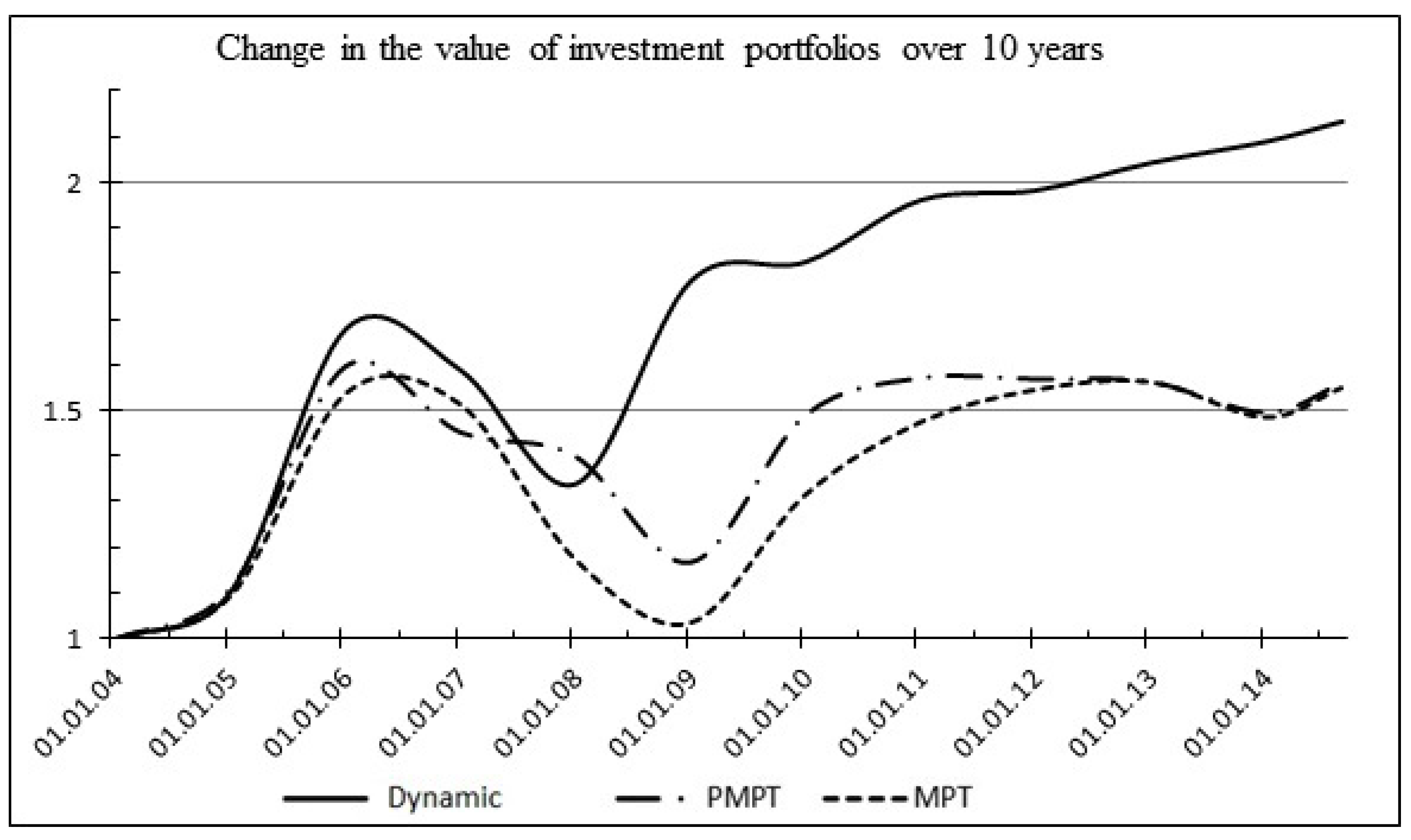
As a result of the experiment, the overall advantage of the dynamic adaptive portfolio was confirmed in comparison with the classical portfolio models of R. Roll and H. Markowitz. The results of modeling (Table 8) and the value change diagram (Figure 15) of investment portfolios are presented below.

Table 8.
Simulation modeling results.
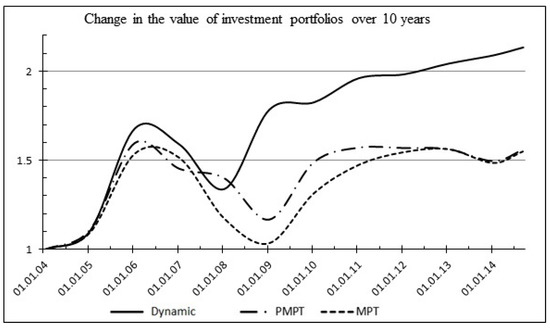
Figure 15.
Simulation modeling results.
4. Discussion and Conclusions
The economically and statistically based model for strategic investment portfolio is developed. It is based on the concept of adaptation strategy to market conditions and modern mathematical instruments. The mathematical instruments are developed. They are necessary for devising the adaptive model of investment portfolios. The components of ensemble forecast of profitability and risk are formalized. The model is reliable due to the fact that the financial market is stochastic. Thus, when the market is stochastic, the model works. This model can be applied to investment portfolio management. The model is stable in terms of crises on the financial market.
The model has limitations. The model cannot be left without observations. It needs constant rebalancing. In addition, the model is computationally complex and cannot be implemented without computer technology. The model does not take into account political and economic pressure, global catastrophes (wars), and demographic factors.
The efficient instrument for long-term forecasting of asset profitability is developed. It is based on mathematical statistics and neural modeling. The created model is empirically evaluated on real data. The model was shown to outperform some standard models in terms of efficiency.
Future research directions may lie in the analysis and selection of various optimization methods for building future forecasts and investment models. For example, higher-order moments can be explored, which may have predictive properties. In addition, moments of higher orders can be studied in the framework of constructing econometric models of the crisis.
Funding
This research received no external funding.
Institutional Review Board Statement
Not applicable.
Informed Consent Statement
Not applicable.
Data Availability Statement
Not applicable.
Conflicts of Interest
The author declares no conflict of interest.
References
- Ivanyuk, V. Formulating the concept of an investment strategy adaptable to changes in the market situation. Economies 2021, 9, 95. [Google Scholar] [CrossRef]
- Ivanyuk, V. Modeling of Crisis Processes in the Financial Market. Economies 2021, 9, 144. [Google Scholar] [CrossRef]
- Statman, M. How many stocks make a diversified portfolio? J. Financ. Quant. Anal. 1987, 22, 353–363. [Google Scholar] [CrossRef]
- Chen, Y.W.; Poon, S.H.; Yang, J.B.; Xu, D.L.; Zhang, D.; Acomb, S. Belief rule-based system for portfolio optimisation with nonlinear cash-flows and constraints. Eur. J. Oper. Res. 2012, 223, 775–784. [Google Scholar] [CrossRef]
- Nikolakakis, T.; Chattopadhyay, D.; Malovic, D.; Vayrynen, J.; Bazilian, M. Analysis of electricity investment strategy for Bosnia and Herzegovina. Energy Strategy Rev. 2019, 23, 47–56. [Google Scholar] [CrossRef]
- Appio, F.P.; De Luca, L.M.; Morgan, R.; Martini, A. Patent portfolio diversity and firm profitability: A question of specialization or diversification? J. Bus. Res. 2019, 101, 255–267. [Google Scholar] [CrossRef]
- Way, R.; Lafond, F.; Lillo, F.; Panchenko, V.; Farmer, J.D. Wright meets Markowitz: How standard portfolio theory changes when assets are technologies following experience curves. J. Econ. Dyn. Control. 2019, 101, 211–238. [Google Scholar] [CrossRef]
- Pezier, J.; Scheller, J. Best portfolio insurance for long-term investment strategies in realistic conditions. Insur. Math. Econ. 2013, 52, 263–274. [Google Scholar] [CrossRef]
- Vo, N.; He, X.; Liu, S.; Xu, G. Deep learning for decision making and the optimization of socially responsible investments and portfolio. Decis. Support Syst. 2019, 124, 113097. [Google Scholar] [CrossRef]
- Akarim, Y.D.; Sevim, S. The impact of mean reversion model on portfolio investment strategies: Empirical evidence from emerging markets. Econ. Model. 2013, 31, 453–459. [Google Scholar] [CrossRef]
- Jadhao, G.; Chandra, A. Application of VIX and entropy indicators for portfolio rotation strategies. Res. Int. Bus. Financ. 2017, 42, 1367–1371. [Google Scholar] [CrossRef]
- Wei, J.; Shen, Y.; Zhao, Q. Portfolio selection with regime-switching and state-dependent preferences. J. Comput. Appl. Math. 2020, 365, 112361. [Google Scholar] [CrossRef]
- Ma, G.; Siu, C.C.; Zhu, S.P. Dynamic portfolio choice with return predictability and transaction costs. Eur. J. Oper. Res. 2019, 278, 976–988. [Google Scholar] [CrossRef]
- Kang, Z.; Zhao, L.; Sun, J. The optimal portfolio of α-maxmin mean-VaR problem for investors. Phys. Stat. Mech. Its Appl. 2019, 526, 120778. [Google Scholar] [CrossRef]
- Dai, Z.; Wang, F. Sparse and robust mean–variance portfolio optimization problems. Phys. A Stat. Mech. Its Appl. 2019, 523, 1371–1378. [Google Scholar] [CrossRef]
- Lu, Y.N.; Li, S.P.; Zhong, L.X.; Jiang, X.F.; Ren, F. A clustering-based portfolio strategy incorporating momentum effect and market trend prediction. Chaos Solitons Fractals 2018, 117, 1–15. [Google Scholar] [CrossRef]
- Jung, Y.C. A portfolio insurance strategy for volatility index (VIX) futures. Q. Rev. Econ. Financ. 2016, 60, 189–200. [Google Scholar] [CrossRef]
- Lin, L.; Zhou, Z.; Liu, Q.; Jiang, Y. Risk transmission between natural gas market and stock markets: Portfolio and hedging strategy analysis. Financ. Res. Lett. 2019, 29, 245–254. [Google Scholar] [CrossRef]
- Liu, Y.J.; Zhang, W.G. Flexible time horizon project portfolio optimization with consumption and risk control. Appl. Soft Comput. 2019, 76, 282–293. [Google Scholar] [CrossRef]
- Chen, J.S.; Hou, J.L.; Wu, S.M.; Chang-Chien, Y.W. Constructing investment strategy portfolios by combination genetic algorithms. Expert Syst. Appl. 2009, 36, 3824–3828. [Google Scholar] [CrossRef]
- Kunitomo, N.; Awaya, N.; Kurisu, D. Comparing estimation methods of non-stationary errors-in-variables models. Jpn. J. Stat. Data Sci. 2020, 3, 73–101. [Google Scholar] [CrossRef]
- Banerjee, A.; Dolado, J.J.; Galbraith, J.W.; Hendry, D. Co-Integration, Error Correction, and the Econometric Analysis of Non-Stationary Data; Oxford University Press: Oxford, UK, 1993. [Google Scholar] [CrossRef]
- Pesaran, M.H.; Shin, Y.; Smith, R.J. Bounds testing approaches to the analysis of level relationships. J. Appl. Econom. 2001, 16, 289–326. [Google Scholar] [CrossRef]
- Johansen, S. Likelihood-Based Inference in Cointegrated Vector Autoregressive Models; Oxford University Press: Oxford, UK, 1995. [Google Scholar]
- Willmott, C.J.; Matsuura, K. Advantages of the mean absolute error (MAE) over the root mean square error (RMSE) in assessing average model performance. Clim. Res. 2005, 30, 79–82. [Google Scholar] [CrossRef]
- Makridakis, S.; Taleb, N. Decision making and planning under low levels of predictability. Int. J. Forecast. 2009, 25, 716–733. [Google Scholar] [CrossRef]
- Kotelnikov, V.A. On the transmission capacity of the ether and of cables in electrical communications. In Proceedings of the First All-Union Conference on the Technological Reconstruction of the Communications Sector and the Development of Low-Current Engineering, Moscow, Russia, 1933; Available online: http://ict.open.ac.uk/classics/1.pdf (accessed on 25 August 2022).
- Shannon, C.E. Communication in the presence of noise. Proc. IRE 1949, 37, 10–21. [Google Scholar] [CrossRef]
- Ivanyuk, V. Developing a crisis model based on higher-order moments. Heliyon 2022, 8, e08896. [Google Scholar] [CrossRef]
Publisher’s Note: MDPI stays neutral with regard to jurisdictional claims in published maps and institutional affiliations. |
© 2022 by the author. Licensee MDPI, Basel, Switzerland. This article is an open access article distributed under the terms and conditions of the Creative Commons Attribution (CC BY) license (https://creativecommons.org/licenses/by/4.0/).


