Phase Analysis of Event-Related Potentials Based on Dynamic Mode Decomposition

Abstract

Real-time detection of event-related potentials (ERPs) and exploration of ERPs generation mechanisms are vital to practical application of brain–computer interfaces (BCI). Traditional methods for ERPs analysis often fall into time domain, time–frequency domain, or spatial domain. Methods which can reveal spatiotemporal interactions by simultaneously analyzing multi-channel EEG signals may provide new insights into ERP research and is highly desired. Additionally, although phase information has been investigated to describe the phase consistency of a certain frequency component across different ERP trials, it is of research significance to analyze the phase reorganization across different frequency components that constitute a single-trial ERP signal. To address these problems, dynamic mode decomposition (DMD) was applied to decompose multi-channel EEG into a series of spatial–temporal coherent DMD modes, and a new metric, called phase variance distribution (PVD) is proposed as an index of the phase reorganization of DMD modes during the ERP in a single trial. Based on the PVD, a new error-related potential (ErrP) detection method based on symmetric positive defined in Riemann manifold is proposed to demonstrate the significant PVD differences between correct and error trials. By including the phase reorganization index, the 10-fold cross-validation results of an ErrP detection task showed that the proposed method is 4.98%, 27.99% and 7.98% higher than the counterpart waveform-based ErrP detection method in the terms of weighted accuracy rate, precision and recall of the ErrP class, respectively. The resulting PVD curve shows that with the occurrence of ERP peaks, the phases of different frequency rhythms are getting to aligned and yields a significant smaller PVD. Since the DMD modes of different frequencies characterize spatiotemporal coherence of multi-channel EEG at different functional regions, the new phase reorganization index, PVD, may indicate the instantaneous phase alignment of different functional networks and sheds light on a new interpretation of ERP generation mechanism.

1. Introduction

Brain activity signals can be broadly classified into spontaneous brain rhythms and event-related potentials (ERPs), where ERPs are evoked by stimuli or events and exhibit stable temporal relationships with deterministic reference events, i.e., they are the time-locked and phase-locked responses of the brain to external stimuli [1]. ERP waveforms consist of multiple components characterized by a particular latency, polarity, shape, amplitude and spatial distribution on the scalp and reflect neuro-electrophysiological processes in the brain during cognitive processes. The early components are triggered by a sensory stimulation, whereas the late components reflect cognitive processing [2]. The exploration of the generation mechanisms as well as real-time detection of these ERPs are vital to applications such as brain–computer interfaces (BCI).

Neural dynamics are well-known to be characterized by dynamic oscillations at many frequency bands, which are implicated in a variety of neural functions [3,4,5,6]. Oscillations can be described in terms of frequency, amplitude and phase, wherein different frequencies reflect different neuronal processing systems, differences in amplitudes reflect the extent of task involvement, and phase indicates the timing of neuronal activity [7]. However, the neurophysiological mechanisms that produce ERPs are less well-understood compared to the neurophysiological mechanisms that produce oscillations, such as the ERD/S phenomena. Whether ERPs are generated by a fixed-latency or fixed-polarity response, as suggested by the evoked model, or by a reset of oscillatory activity, as predicted by the phase reset model, is still a question worth exploring [8,9,10,11]. Beyond the evoked and phase-reset model, the event-related phase reorganization (ERPR) model [9] gives the view that instantaneous event-related alignment in phase between task-relevant frequencies produces ERPs.

Phase information has been investigated before in the context of ERPs in theta and alpha bands [12,13,14,15]. Oscillatory activity in theta and alpha bands revealed that instantaneous phase patterns can contain information about the response to external stimuli (visual or auditory event-related potentials) [14]. Specifically, the instantaneous phase value at every time–frequency point in the ERP data of a single trial can be calculated by continuous wavelet transform, short-time Fourier transform or Hilbert transform, and then the phase consistency at different time–frequency points can be quantitatively measured by the inter-trial phase clustering (ITPC) method [16], which is indexed by the summation of phase angles of all epochs. However, most of the phase information of ERPs in the existing literature refers to the extent of phase consistency at the same time–frequency point across different trials; it may also be of research significance to analyze the phase consistency across different frequency components that constitute the single-trial ERP signal.

ERPs signals are often embedded in strong stimulus-independent spontaneous electroencephalography (EEG) activity and environmental noise, and the low signal-to-noise ratio makes the analysis and classification of ERPs based on single trial still challenging. Although the widely used Fourier transform is capable of transforming a single-channel time-varying EEG signal to a spectrum in order to capture the frequency information of ERPs, it is still expected that methods that can analyze multi-channel EEG signals simultaneously in the spatial and time domains may provide new perspectives and information for ERP research. One example of a modal decomposition in time that goes beyond the Fourier transform is empirical mode decomposition (EMD) [17], which computes intrinsic oscillatory modes from time-varying data and has been used to analyze neural data, including cortical local field potential and EEG [18,19]. A relatively new modal decomposition method called dynamic mode decomposition (DMD) [20,21] has been proposed based on the Koopman operator theory [22] to study complex nonlinear dynamics in a linear observable space, which was first implemented in the fluid mechanism. DMD was initially introduced to reduce very high-dimensional dynamic data into relatively few coupled spatial–temporal modes. In the context of analyzing neural recordings, DMD was first introduced to be a novel approach to explore spatial–temporal patterns in large-scale neural recordings; the analysis results on electrocorticography (ECoG) data finally validated the view that DMD modes can be thought of as coherent structures in the neural activity [23,24,25,26]. Since EEG comprises well-known nonlinear and non-stationary signals, decomposing and representing EEG in low-dimensional DMD modal space can comprehensively characterize brain dynamics and may reveal ERP activities superimposed on the background EEG.

In this paper, DMD was firstly applied to decompose ERP signals into a series of spatial–temporal coherent DMD modes, and then a new metric called PVD, which quantifies the phase consistency of all DMD modes during time-evolution process in a single trial, was proposed. Based on the view that instantaneous event-related alignment in phase generates ERPs, this paper assumes that the DMD modes with differently fixed frequency can be used to describe the oscillation activities in the EEG dynamics, then at the time point when the ERPs peak occurs, the phases of oscillations of different frequency are aligned, and the value of PVD will decrease, while during the non-ERP peak time, the value of PVD is close to 1, indicating that the phase difference of each DMD mode is large. Furthermore, a binary ERP classification method based on the PVD metric and Riemann approach was proposed to demonstrate the effect of the intra-trial phase consistency on ERP detection.

2. Materials and Methods

2.1. Data Acquisition and Preprocessing

The ERP dataset chosen in this work is the monitoring error-related potential dataset [27], containing two-session recordings of six subjects which are separated by several weeks, and each experimental session consists of 10 blocks, each of which contains approximately 50 trials and lasts approximately 3 min. Specifically, when subjects realize that they have made an erroneous operation or that there is an error in the behavior of an external device that they are observing, the brain generates event-related potentials associated with the error, called error-related potentials (ErrPs) [28]. A stable ErrP waveform can be detected within 500 ms after the subject feels the error-related event, including an initial short negative deflection, followed by a short positive deflection, and finally a longer negative wake [29]. ErrP has been shown to be an inherent feedback mechanism of humans, meaning that ErrP can be elicited in the human brain untrained and naturally in the event of an error. EEG potentials were recorded at full DC at a sampling rate of 512 Hz for all subjects using a Biosemi ActiveTwo system, and the 64 electrodes were placed according to the extended 10/20 international system. During the experiment, subjects were seated in front of a computer and stared at the screen where a moving cursor and a target location were displayed. At each trial, the cursor moved horizontally toward the target location for about 2 s; after reaching the target, the cursor remained in place and a new target was drawn no more than 3 positions away from the current cursor position. During the trial, subjects had no control over the cursor movement and were only asked to monitor the performance of the cursor. To elicit an ErrP signal, the probability of the cursor moving in the wrong direction (opposite the target position) was approximately 20% in each trial.

In this work, the ErrPs signals were filtered with a Butterworth bandpass filter of order 4 within the band [0.1, 20] Hz as in [30] (the Butterworth filter is an infinite impulse response (IIR) filter and the IIR filter transform can filter or attenuate undesired frequency (spectrum) components presented in the EEG data), and downsampled from 512 Hz to300 Hz for computational efficiency. Then the signal was spatially filtered with common average reference (CAR) [31]. Taking the beginning time step of the event (correct or erroneous movement of the cursor) as 0 s, we segmented [−200, 800] ms of each recording block as an epoch and used the data of [−200, 0] ms to remove the baseline. A preprocessed epoch has a dimension of $64\times 300$, and further signal analysis was based on the epochs. There were about 500–600 samples per session of each subject, in which the ratio of ErrPs trials and non-ErrPs trials was about 1:4. All above processes were implemented with the MNE Python package [32].

2.2. Computation of the Dynamic Mode Decomposition

In this study, a DMD method which is used to extract the functional connectivity and the synchronization of the functional networks will be further studied and used to detect ErrPs. Usually, the EEG signal recorded on the scalp is a multi-channel time series that can be expressed as a two-dimensional matrix. The number of time points contained in the signal matrix is denoted as M, and the number of measurements per time step, i.e., the number of electrodes, is denoted as N. Hence, the signal matrix is expressed as follows:

$$X=\left. [\begin{array}{cccc}|& |& & |\\ x_0& x_1& \dots & x_M\\ |& |& & |\end{array}\right]=\left. [\begin{array}{ccc}{u}_1\left(t_0\right)& \cdots & u_1\left(t_M\right)\\ ⋮& \ddots & ⋮\\ u_N\left(t_0\right)& \cdots & u_N\left(t_M\right)\end{array}\right],$$

(1)

where $x_0,x_1,\dots ,x_M$ are sample vectors uniformly sampled along the time dimension, with $x_k$ denoting the vector of measurements at time k, and $k=1,2,\dots ,M$. $u_i\left(t_j\right)$ is the value on the ith electrode at the jth time step.

DMD was originally used in the study of large fluid flow fields, where typically, the data matrix has the characteristic of $N>>M$. In contrast, in neuroscience for the recorded EEG signal data, the number of sampling time points is often much larger than the number of electrodes. Therefore, the following augmented matrix $X_{aug}$ needs to be constructed according to the original EEG matrix X before applying DMD [24], appending to the snapshot measurements with $h-1$ time-shifted versions of the original matrix, thus augmenting the number of measurements to be $hN$:

$$X_{aug}=\left. [\begin{array}{cccc}{x}_1& x_2& \cdots & x_{M-h}\\ x_2& x_3& \cdots & x_{M-h+1}\\ ⋮& ⋮& \ddots & ⋮\\ x_h& x_{h+1}& \cdots & x_{M-1}\end{array}\right],$$

(2)

where h is a minimum integer that satisfies $h<\frac{M+1}{N+1}$.

According to the Koopman operator theory, a finite dimensional nonlinear dynamic system can be represented by a linear system in an infinite dimensional observable space. DMD gives an effective approximation to the infinite observable space. Gathering measurements from M electrodes in time, two $hN\times \left(M-h-1\right)$ EEG data matrices can be constructed as follows:

$$\begin{array}{c}{X}_{aug}=\left. [\begin{array}{cccc}|& |& & |\\ x_0& x_1& \dots & x_{M-1}\\ |& |& & |\end{array}\right]\hfill \\ {X_{aug}}^{\prime }=\left. [\begin{array}{cccc}|& |& & |\\ x_1& x_2& \dots & x_M\\ |& |& & |\end{array}\right]\hfill \end{array}.$$

(3)

Note that $X_{aug}$ and ${X_{aug}}^{\prime }$ contain largely overlapping data, differing in that columns of ${X_{aug}}^{\prime }$ are shifted one time step from those in $X_{aug}$. The locally linear dynamics can be denoted as [24]:

$${X_{aug}}^{\prime }=A{X}_{aug}.$$

(4)

Therein, A is the optimal linearization matrix that can transform matrix $X_{aug}$ into ${X_{aug}}^{\prime }$, called the DMD operator. The best-fit DMD operator can be solved by

$$A={X_{aug}}^{\prime }{X_{aug}}^{†},$$

(5)

where ${X_{aug}}^{†}$ is the Moore–Penrose pseudoinverse of $X_{aug}$. To reduce the computational complexity, one possible approach is to perform singular value decomposition (SVD) of the matrix $X_{aug}$:

$$X_{aug}\approx U\sum V^{\ast },$$

(6)

where $V^{\ast }$ represents the conjugate transpose of V, $U\in {\mathbb{C}}^{hN\times (M-h-1)}$, $\sum \in {\mathbb{C}}^{(M-h-1)\times (M-h-1)}$ and $V^{\ast }\in {\mathbb{C}}^{(M-h-1)\times (M-h-1)}$. According to the similarity matrix properties, the high-dimensional matrix A is transformed to a low-dimensional matrix $\tilde{A}$ as

$$\tilde{A}=U^{\ast }{X_{aug}}^{\prime }V\sum ^{-1}.$$

(7)

The eigenvector of matrix $\tilde{A}$ is calculated by

$$\tilde{A}W=W\mathsf{\Lambda }.$$

(8)

where each column of the matrix W is the eigenvector of the matrix $\tilde{A}$, the matrix $\mathsf{\Lambda }$ is a diagonal matrix of eigenvalues ${\lambda }_i$ which are corresponding to the eigenvectors. Each eigenvalue ${\lambda }_i$ is a DMD eigenvalue. The DMD mode matrix $\mathsf{\Phi }$ can be obtained by mapping matrix W back to the high-dimensional observable space by

$$\mathsf{\Phi }={X_{aug}}^{\prime }V{\Sigma }^{-1}W.$$

(9)

Each column of $\mathsf{\Phi }$ is a DMD mode ${\phi }_i$ corresponding to the eigenvalue ${\lambda }_i,i=1,\dots ,M-h-1$. The absolute values and phases of $\mathsf{\Lambda }$ are the decay rates and frequencies, respectively. Specifically, the frequencies corresponding to DMD modes are given as

$$f=\frac{imag\left(ln\left(\lambda \right)/\mathsf{\Delta }t\right)}{2\pi },$$

(10)

where $\mathsf{\Delta }t$ is the sampling interval between two sample points. Once the eigenvalues and eigenvectors of the linear transformation matrix A of the discrete linear system are obtained, the original EEG signal can be reconstructed from the DMD modes as [24]

$$x\left(t\right)\approx \sum _{k=1}^r{\phi }_{k}exp\left(w_{k}t\right)b_k=\mathsf{\Phi }exp\left(\mathsf{\Omega }t\right)\mathbf{b},$$

(11)

where r is the number of DMD modes, $\mathsf{\Omega }=ln\left(\mathsf{\Lambda }\right)/\mathsf{\Delta }t$ and $\mathbf{b}$ is a dialog matrix composed of a set of coefficient to match the first time point measured such that $x\left(1\right)=\mathsf{\Phi }\mathbf{b}$, which are also known as the participation factor of each DMD mode. It should be noted that $\mathsf{\Phi }$ and $\mathsf{\Omega }$ are sets of vectors with complex values, as shown in Figure 1a.

DMD modes correspond to correlations in space at frequencies dictated by the DMD eigenvalues. As shown in Figure 1b) Formula (10) indicates that the raw EEG data can be decomposed into a sum of DMD modes, each of which has a spatial part and a temporal evolution part. The spatial modes can be readily interpreted as relative magnitudes of correlation among electrodes, and the phase components of these spatial modes can be interpreted as relative synchrony between electrodes [33]. Notably, the spatial patterns extracted as DMD modes with coherent dynamics at a particular frequency band are comparable, but not identical, to spatial patterns extracted by band-pass filtering each channel of recording at the same frequency band. DMD eigenvalues are complex valued so that the dynamics have growth/decay in addition to frequency of oscillation. This ability to capture growth/decay of spatial patterns is important when analyzing nonstationary signals and transient behaviors.

2.3. Analysis for Phase Information of DMD Modes

Brain oscillation theory offers an alternative explanation for the generation of ERP components, which is different from that of the evoked model. The interpretation of the event-related EEG response is a logical consequence from results obtained for the ongoing EEG. Oscillations reflect different sensory and cognitive processes and play an important role in the timing of neural processes also for the event-related EEG response. The event-related phase reorganization (ERPR) [9] model gives the view that instantaneous event-related alignment in phase between task relevant frequencies produces ERPs. Specifically, an ERP generated by ERPR can be understood as the sum of instantaneous amplitudes a of different task-relevant frequencies w at time point t, averaged over trials k:

$$ERP(phase-reorganization)=\sum _{y}a\left(w_y,t_x\right),$$

(12)

where $t_x$ refers to the xth time point, and y denotes the index of a trial. For the optimal processing of a stimulus, phase reorganization is obligatory, which does not mean a phase reset, but instantaneous phase alignment (IPA) [9]. ERP components are determined by IPA; reset and/or IPA takes place not necessarily at the positive or negative peak.

Instantaneous phase alignment can also be understood as the consistency of phases at different time–frequency points, which correspond to a series of oscillatory activities with different frequencies. The phase angle which is usually represented as a cyclic quantity in the interval $\left. [-\pi ,\pi \right]$ lies on the $S^1$ manifold. Therefore, the phase angles cannot be simply summed and averaged using the operators defined in the 1-dimensional Euclidean space. Euler’s formula provides a mapping between the angle and the vector in the complex plane, that is, $e^{i\theta }=cos\theta +i·sin\theta$. Hence a cluster of phase angles can be represented as a cluster of vectors on the unit circle. Inter-trial phase clustering (ITPC) [16] defines a metric for quantifying event-related phase modulations as

$$ITP{C}_{tf}=\left|\frac{1}{n}\sum _{r=1}^n{e}^{i{k}_{tfr}}\right|,$$

(13)

where n is the number of trials; $e^{ik}$ is Euler’s formula, which represents the complex vector corresponding to the local phase angle with the value k in radians at the time–frequency point $tf$ in the rth trial; and $|·|$ indicates the length of the averaged vector. An ITPC value close to 0 reflects high variability of the phase angles across trials, whereas an ITPC value of 1 reflects all trials having the same phase angle.

EEG recordings containing ERPs can be decomposed as a linear sum of a series of DMD modes with fixed oscillation frequencies and fixed decay or growth rates, i.e., DMD extracts the frequencies of oscillations observed in the measurements. The magnitude of each element in a certain DMD mode vector can be interpreted as the functional connectivity, which represents relative amplitudes of correlation among electrodes. The phase of each element in a certain DMD mode vector can be interpreted as the relative synchronization relationship between different electrodes. A row vector in the DMD modes matrix represents the decomposition result of the EEG signal recorded at a specific electrode, namely, the decomposition of the temporal evolution of the EEG channels as the combination of brain oscillation activities with different frequencies which generate ERPs. Therefore, an IPA among the temporal evolution of various DMD modes can be defined. Unlike the ITPC studying the phase clustering across trials, a new metric which describes the phase consistency among all DMD modes in a single trial can be defined. In this paper, the phase variance distribution of DMD modes (PVD) at a certain electrode is proposed to measure the phase consistency of different modes in a single trial. The phase vector of all modes at specific time t can be calculated as $angle\left({\varphi }_n·exp\left(\mathsf{\Omega }t\right)·\mathbf{b}\right)$ and the PVD of channel n can then be defined as

$$PV{D}_n\left(t\right)=\mathbf{var}\left(exp\left(j·angle\left({\varphi }_n·exp\left(\mathsf{\Omega }t\right)·\mathbf{b}\right)\right)\right),$$

(14)

where t is the time of a single trial, and in this paper $t\in \left. [-0.2s,0.8s\right]$, j represents complex number, n denotes the nth electrode and $n=1,\dots ,N$, ${\varphi }_n$ denotes the nth row vector of the DMD mode matrix $\mathsf{\Phi }$, and $exp\left(\mathsf{\Omega }t\right)·\mathbf{b}$ is the matrix containing all of the time evolution of each mode. The operator $\mathbf{var}$ calculates the variance of the corresponding complex values based on the Euclidean distance. PVD(t) calculates the variance of the phase vectors in the time evolution process of DMD modes that compose the measured EEG signal on a certain EEG electrode within a single trial. Hence, PVD represents the evolution trend of the phase variance among the DMD modes during the ERP. Based on the ERPR model, at the time point when the ERP peak occurs, the phases of oscillations of different frequency are aligned and the value of PVD will decrease, indicating the instantaneous phase alignment. During the non-ERP peak time, the value of PVD is close to 1, indicating that the phase difference of each DMD mode is large. Based on this hypothesis, the PVD values will be used to discriminate the ErrP trial from non-ErrP trials without using multiple trial averaging.

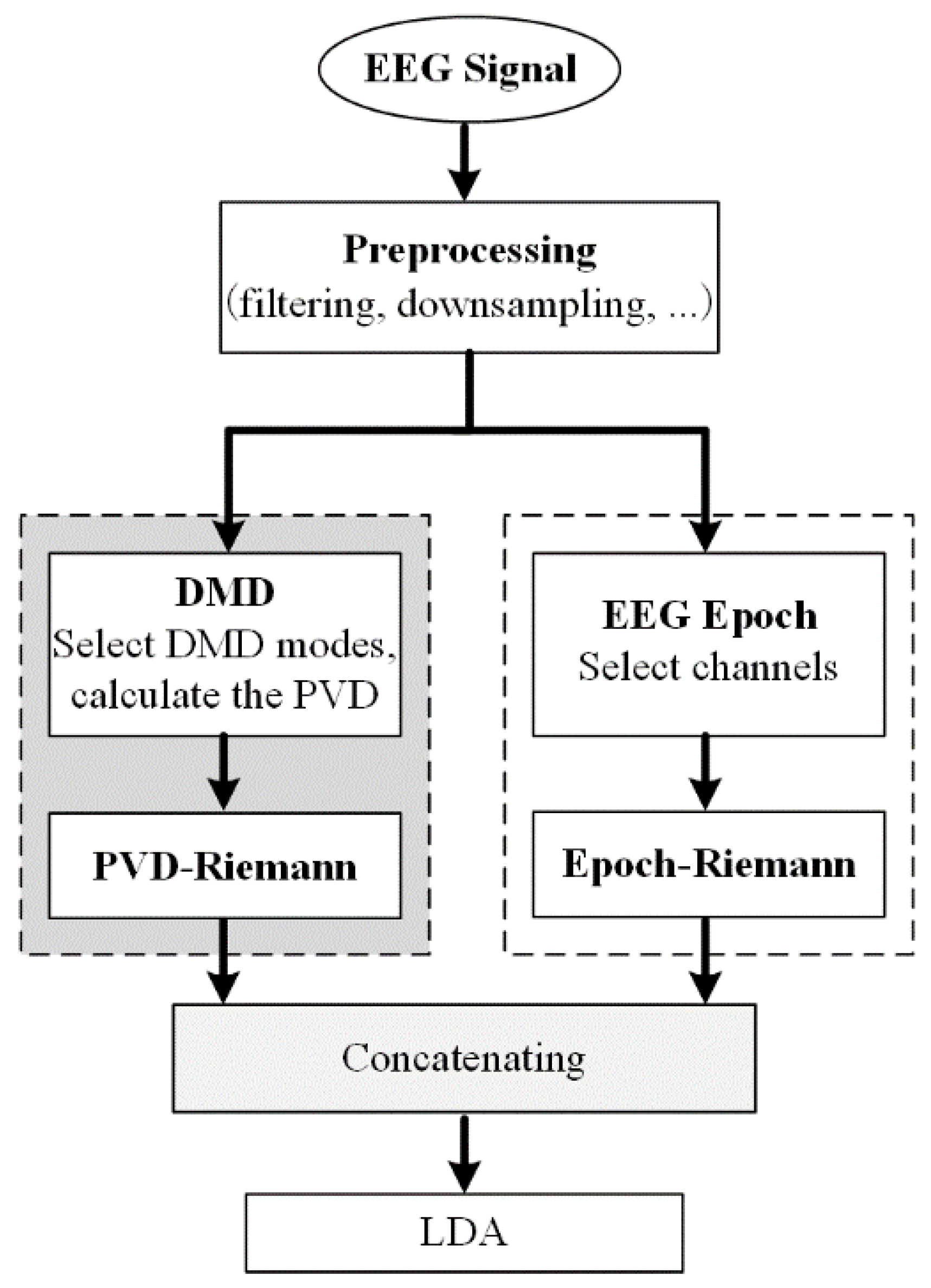
2.4. Classification Based on DMD Phase Information and Riemann Approach

Different sources of neural activity project at the scalp with a specific distribution. Spatial covariances between EEG channels capture the shape of this distribution and the strength of the activity averaged across the time-window of interest [34]. For $X\in {\mathbb{R}}^{n\times s}$ a multi-channel segment of EEG signal and a template signal, the following template-signal covariance matrix can be built as [35]

$$C=\frac{1}{s}Z{Z}^T=\frac{1}{s}\left(\begin{array}{cc}T{T}^T& T{X}^T\\ X{T}^T& X{X}^T\end{array}\right),$$

(15)

where n is the number of channels, s is the number of sample points, and $Z=\left. [\begin{array}{cc}X& T\end{array}\right]\in {\mathbb{R}}^{s\times 2n}$. Formula (15) indicates that the original epoch EEG datum X is augmented with a template T along the channel dimension to build a super epoch Z. In the context of ERP experiments, the template is typically an average ERP of one or several classes. Unlike the simpler covariance matrix $C=\frac{1}{s}X{X}^T$, the template–signal covariance is capable of extracting the sample information on the off-diagonal blocks and reflecting how similar a particular epoch is to the template dynamics.

The symmetric positive-definite covariance matrices lie on the symmetric positive-definite (Sym+) Riemannian manifold [36]. The Riemann metric provides a measure of distance between SPD matrices along the Riemannian manifold. Based on the Riemann metric, classifiers that directly use SPD matrices as input can be built [37]. However, many classification algorithms, such as linear discriminant analysis (LDA) and support vector machine (SVM), accept vectors as input [38]. The SPD matrices can further be vectorized, as feature vectors and traditional classifiers can be used for the manifold-valued input.

For a Riemannian manifold, there exists a pair of mapping transporting points from the manifold to an attached tangent space and vice versa [39]. Since the tangent space is a Euclidean space, the well-defined mapping allows to leverage the standard vector-based algorithms. Precisely, the geometric mean $\overline{C}$ of the sample of SPD matrices is first computed as

$$\overline{C}=arg\underset{C}{min}\sum _{i=1}^N{\delta }^2\left(C_i,C\right),$$

(16)

where $C_i$ denotes an SPD matrix, and $\delta$ is the Riemannian distance between SPD matrices. The relationship between SPD matrices can be approximated with Euclidean geometry around the geometric mean $\overline{C}$ by projecting them on a tangent space ${\mathbf{S}}_{\overline{C}}$ by logarithmic mapping

$${\mathbf{S}}_{\overline{C}}=Logm\left(C\right)={\overline{C}}^{1/2}logm\left({\overline{C}}^{-1/2}C{\overline{C}}^{-1/2}\right){\overline{C}}^{1/2},$$

(17)

where logm denotes the logarithm of a matrix. Then each SPD matrix $C_i$ is projected on the tangent space of the Riemannian manifold at point $\overline{C}$.

The matrix on the tangent space can further be vectorized by removing the redundant elements as

$$s_i=upper\left({\overline{C}}^{-1/2}{log}_{\overline{C}}\left(C_i\right){\overline{C}}^{-1/2}\right),$$

(18)

where $upper$ is an operator that keeps the upper triangular part of a symmetric matrix and vectorizes it by applying a weight of 1 for elements on the diagonal and a weight of $\sqrt{2}$ for off-diagonal elements. The resulting $s_i$ is a vector and has dimension $n\left(n+1\right)/\phantom{\left(n+1\right)2}2$ (with n the number of rows/columns of the SPD matrices).

In this paper, two types of feature vectors are computed for the ErrPs binary classification: (1) Epoch–Riemann, which are covariance matrices estimated on super EEG epochs augmented with the averaged ERPs, which were estimated from the training data. Here, only the signals on Cz, Fz and FCz channels, which are in the fronto-central areas, are considered [27]. Hence, the size of the augmented covariance matrix is $6\times 6$ and the size of the feature vector projected on a corresponding tangent space is $1\times 21$. (2) The second type of vector is defined based on a PVD–Riemann, that is, the covariance matrices estimated on super PVD epochs augmented with the averaged PVD of ERPs, which were also estimated from the training data. Here, the DMD modes with frequency in 2–12 Hz are included to calculate the PVD, and again only the PVDs on the Cz, Fz and FCz channels are considered to form the covariance matrix. The size of the augmented covariance matrix is $6\times 6$, and the size of the projected feature vector is $1\times 21$. Finally, we concatenate these two feature vectors to obtain the final $1\times 42$ feature vector for classification. The two types of feature vectors characterize the similarities between the EEG channels and the template ERPs in waveform and IPA, respectively.

In this study, a simple linear discriminant analysis (LDA) [40] classifier is used to classify erroneous from correct trials with the concatenated feature vectors as input. The LDA method is to find an optimal projection so that the distance between samples of the same classes is smaller, and the distance between samples of different classes is larger in the projected space. LDA can provide the optimal and highly robust classification when the two classes follow a Gaussian distribution and have equal covariances. In the binary classification problem, LDA is equivalent to least squares regression, and its objective function is as follows:

$$w=arg\underset{w}{max}\frac{tr\left(w^T{S}_{b}w\right)}{tr\left(w^T{S}_{w}w\right)},$$

(19)

where $tr\left(·\right)$ represents the trace of a matrix, $S_b$ is the between-class scatter matrix, and $S_w$ is the within-class scatter matrix. By solving the largest eigenvalue of ${S_w}^{-1}{S}_b$ and the corresponding eigenvector, the projection vector w is obtained; let b be the bias term, $x_i\in {\mathbb{R}}^{\left(n\times m\right)\times 1}$ be the ith sample vector, where n is the number of channels and m is the number of sampling points, and then the LDA decision function is as follows:

$$y=sign\left(w^T{x}_i+b\right)$$

(20)

After the classifier model parameters are determined, the LDA has a faster discriminating speed than complex neural networks for a new incoming feature vector of the EEG signal. The overall flowchart of the classification method based on DMD phase information and Riemann approach is shown in Figure 2.

3. Results

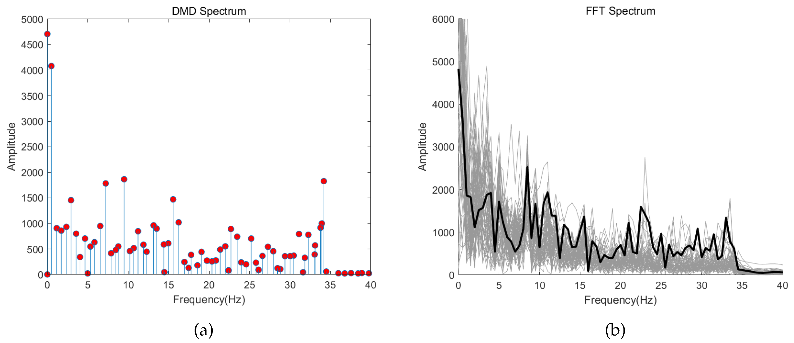
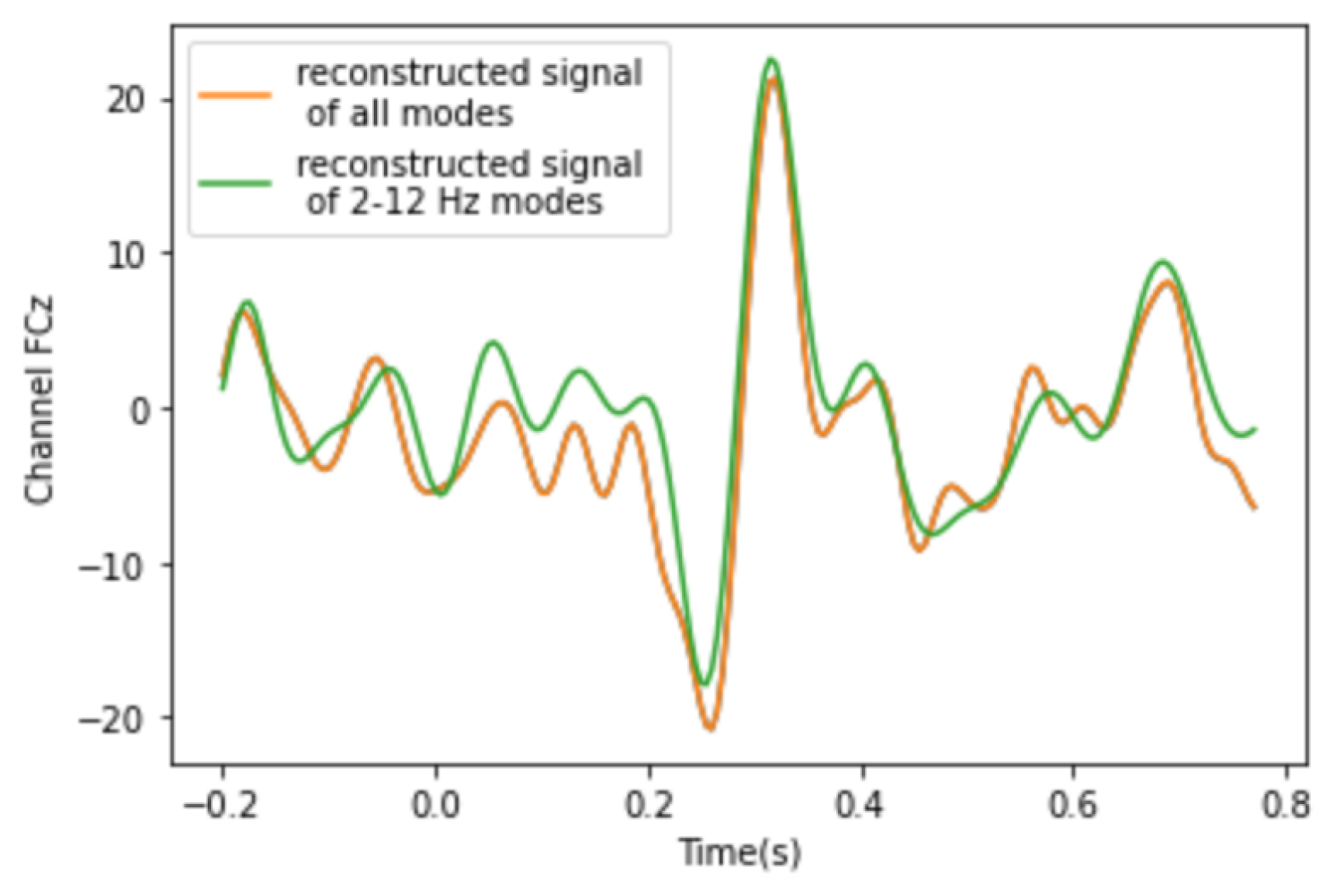
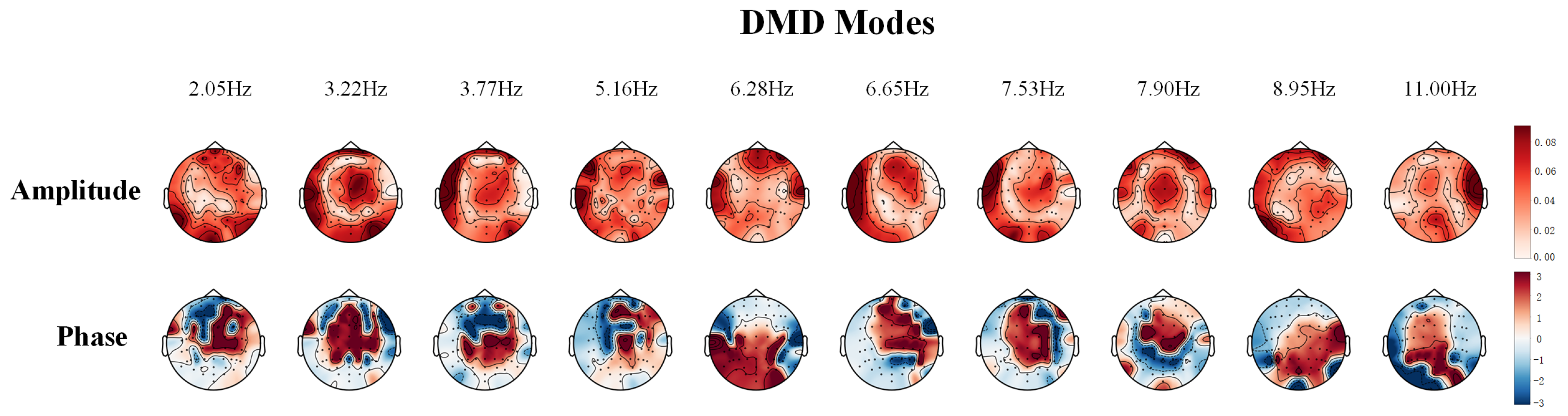
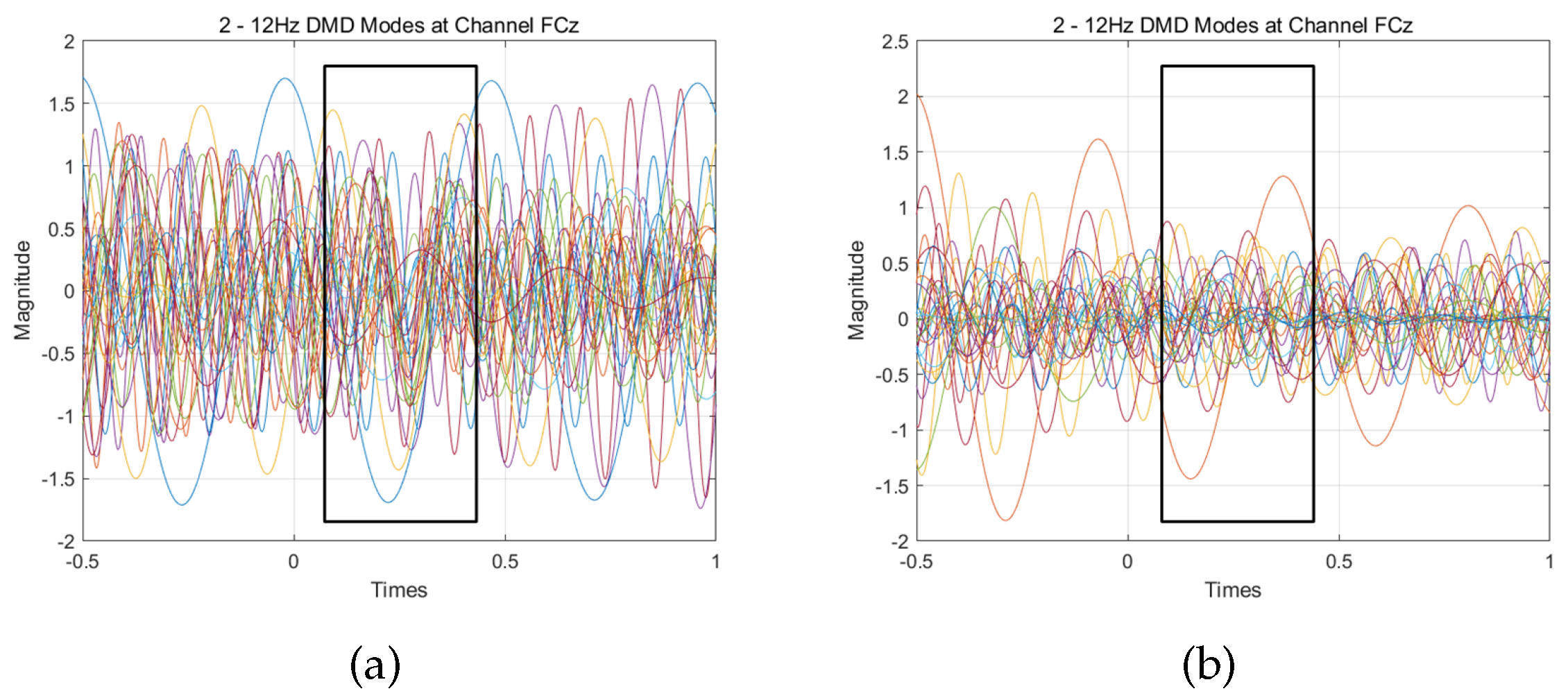
3.1. Analysis of DMD Modes

Take the recording in session 2 of subject 3 in the monitoring error-related potentials dataset as an example and apply DMD to it. Each DMD mode obtained by decomposition has a fixed oscillation frequency, and the energy of all DMD modes can be calculated as $P=diag\left({\mathsf{\Phi }}^T\mathsf{\Phi }\right)$. Figure 3 shows the DMD mode power spectrum distribution at different frequencies and the power spectrum calculated by the fast Fourier transform (FFT). The two are qualitatively similar and have the same rough amplitude decay as frequency increases, which further indicates the accuracy and validity of the DMD modes of the EEG signals. However, the frequencies of the DMD modes are calculated based on all channels of EEG data simultaneously to obtain a sparse and discrete frequency spectrum, which reveals the spatiotemporal coherent properties of brain activity, whereas the FFT is computed based on each electrode’s voltage trace separately. Namely, the DMD spectrum reflects the energy of each mode, which represents the functional network of a specific frequency rather than the energy of the EEG signals.

Although the range of frequencies of DMD modes is large, the mode power distribution is concentrated in the lower frequency band, which is closely related to the ERPs. Reconstructing the original signal by selecting only the DMD modes in lower frequency band, Figure 4 shows the reconstructed signal of all modes and the reconstructed signal of 2–12 Hz modes at the FCz channel, which also indicates the small error between the original and the reconstructed signals by DMD. It can be observed that the DMD modes in the 2–12 Hz frequency range can well-characterize the staple waveform traits of ErrPs. Even if DMD decomposition can obtain a series of spatial–temporal coherent mode patterns, only a small number of important modes which are closely related with the generation of ERPs were selected for further ERP analysis.

The number of all DMD modes with frequencies directly obtained is about 50, while the number of DMD modes that fall in the 2–12 Hz frequency band is only about 12, which indicates that a small number of important modes are sufficient to describe the ERP dynamics of a high-dimensional EEG signal. The DMD modes matrix being a complex matrix reveals that the phase difference among different channels is not constant, and there are traveling waves. The distribution of the amplitude and phase of DMD modes in the frequency range of 2–12 Hz is visualized, as shown in Figure 5. The DMD method can decompose the multi-channel EEG data containing ERPs and obtain relatively few accurate and effective mode activities. Therefore, based on DMD, the patterns in the time, frequency and spatial domain can be comprehensively extracted, which is of high value for subsequent analysis.

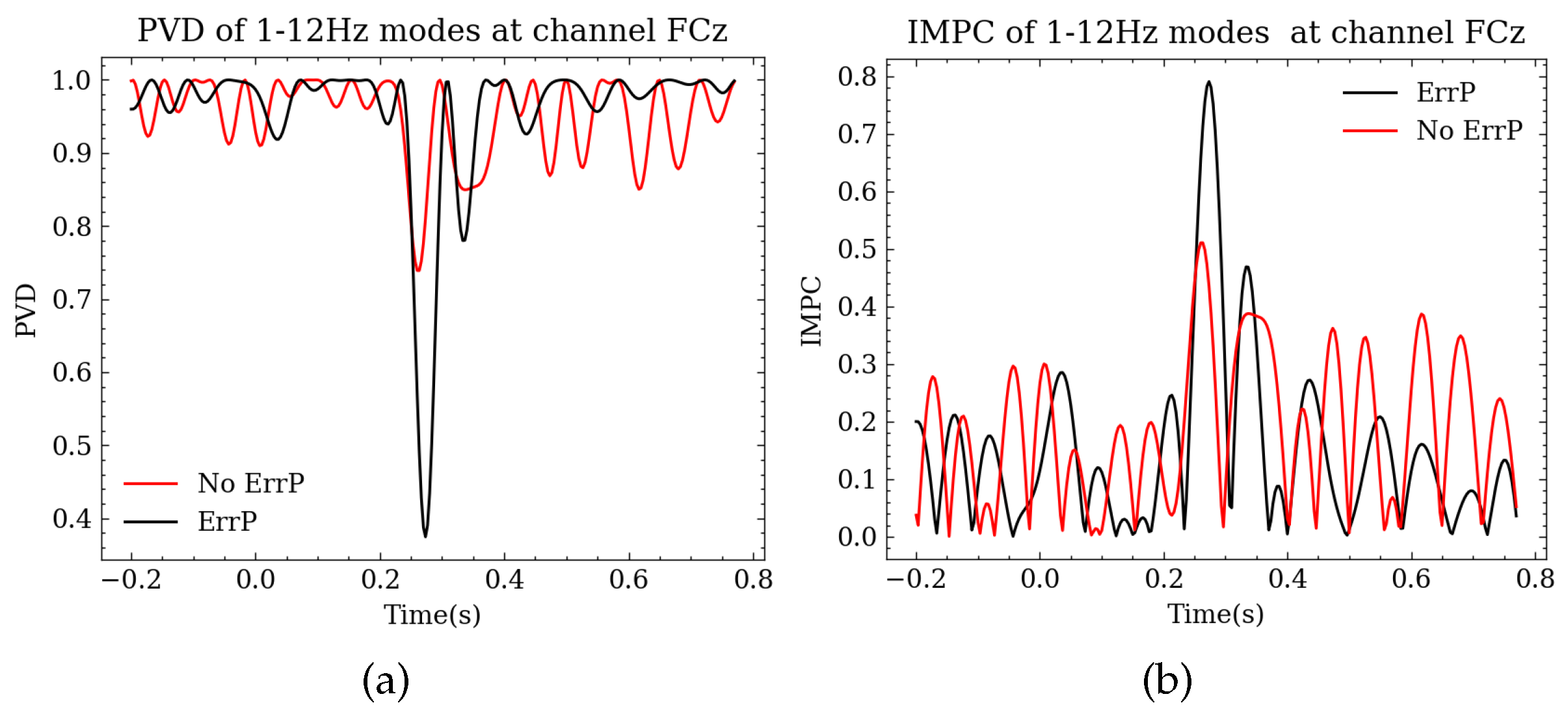
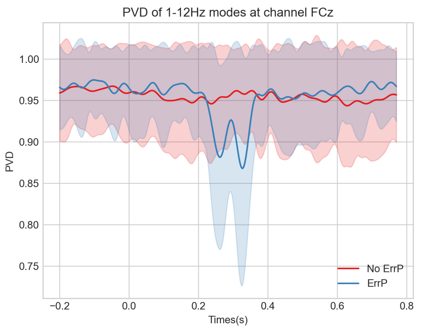
3.2. Analysis of PVD

Take the recordings in session 2 of subject 3 in the monitoring error-related potentials dataset as an example and apply DMD. Figure 6 presents the time course of DMD modes in 2–12 Hz at the FCz channel. Figure 6a refers to the results of the erroneous trial, i.e., containing ErrP, and Figure 6b indicates the correct trial without ErrP. Observing the evolution process of each DMD mode at the FCz channel over time as shown in (a), it can be roughly seen that the phases of the modes of each frequency are relatively synchronously aligned when ERP is generated (inside the black frame), compared to (b) without ERP in the same 0–500 ms time period, while the phases of each mode have no relatively obvious alignment phenomenon.

Figure 7a shows the PVD curve among the time evolutions of 2–12 Hz DMD modes of ERP and no-ERP data at the FCz channel. The PVD of ERP data in the 0.2–0.4 s time period is significantly decreased, indicating a smaller dispersion of the phase angle values among DMD modes, that is, the instantaneous phase alignment of the DMD modes. The results show that the modes obtained by DMD can accurately characterize the EEG temporal dynamics to a certain extent, and the ERP dynamics can be interpreted as the IPA among the various DMD modes. Figure 7b also presents the temporal trend of inter-mode phase consistency (IMPC), which is calculated in a similar way to ITPC, among the time evolutions of 2–12 Hz DMD modes of ERP and non-ERP data at the FCz channel, respectively. It can be seen from the figure that during 0.2–0.4 s, the IMPC value of ERP data is larger than the other time range, indicating that the degree of phase consistency among DMD modes of 2–12 Hz at this time is higher compared with other time periods. The IMPC value of the ERP data within 0.2–0.4 s is larger than the IMPC value of non-ERP data, and the IMPC value of each frequency component of the non-ERP data has no significant difference in the entire time range. Moreover, Figure 8 shows the average curve of the PVD among the time evolutions of 2–12 Hz DMD modes calculated from all trials of subject 3 in the public data set. The results show that the variance-based measure for phase consistency, i.e., PVD, has statistical significance.

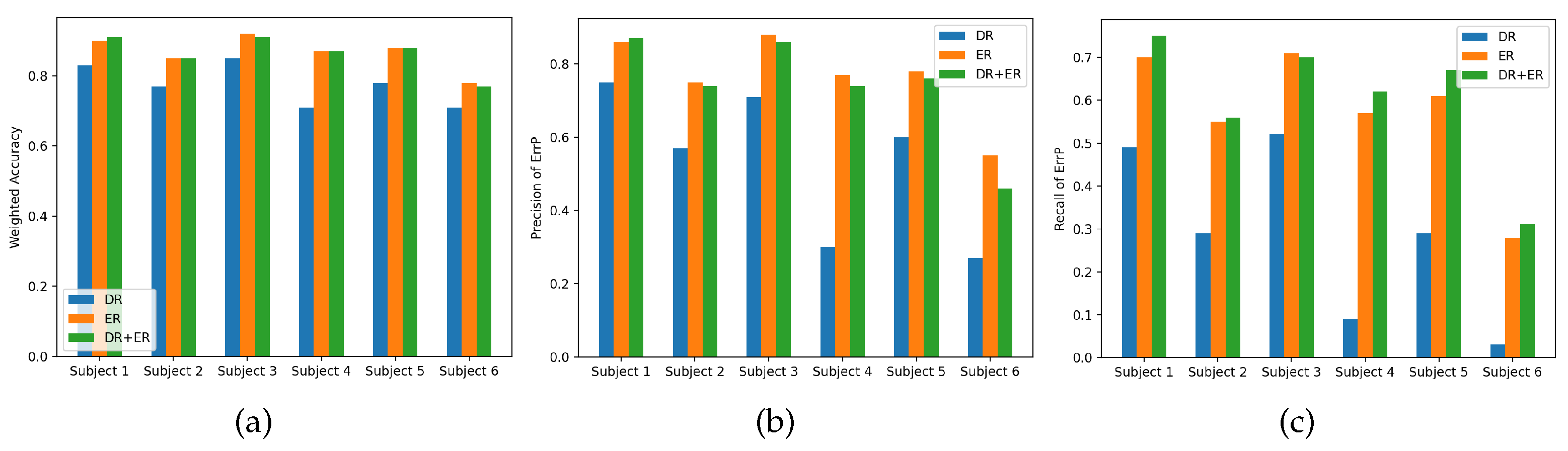
3.3. Performance of ErrP Classification Based on PVD

In this section, the PVD will be used to detect ErrPs to illustrate the effectiveness of the PVD in single-trial ErrP detection. We denote the classification method mentioned in Section 2.4 as the DMD+Riemann classifier. In order to demonstrate the performance of the proposed method, the new method is compared with the common spatial patterns (CSPs) [41] and waveform method [30], which have been reported as being effective in ErrP classification. The CSP method is a spatial filtering feature extraction algorithm for two-classification tasks, which can extract the spatial distribution components of each class from multi-channel EEG data. This experiment refers to the practice in [41] that utilizes 6 electrodes (AF3, AF4, F7, F8, FCz, and CPz) and keeps the two most important components for the CSP. The waveform method is to directly concatenate the processed EEG signals recorded on several key electrodes into a vector as input fed into classifier. Referring to the method in [30], specifically, the EEG data are first downsampled from 300 Hz by a factor of 8, and then the data on the 5 midline electrodes (Fz, FCz, Cz, CPz and Pz) within the time interval of [0.15, 1] s after the event onset are concatenated to obtain the final feature vector. In this experiment, the data of each session of each subject in the monitoring error-related potentials dataset are separately trained and tested. Ten-fold cross-validation is adopted and the average classification prediction results are reported. It is ensured that the ratio of ErrPs trials and non-ErrPs trials in each fold is consistent. The classification results are shown in

Table 1. Comparison of the classification performance of CSP, waveform and DMD+Riemann on the data of each session of each subject. (Average results of 10-fold cross-validation are reported.)

Subject	Session	CSP+LDA			Waveform+LDA			DMD+Riemann
		wAcc	Precision	Recall	wAcc	Precision	Recall	wAcc	Precision	Recall
1	1	0.70	0.22	0.09	0.88	0.77	0.74	0.91	0.87	0.75
	2	0.77	0.38	0.14	0.91	0.85	0.73	0.93	0.88	0.78
2	1	0.73	0.38	0.35	0.79	0.54	0.48	0.85	0.74	0.56
	2	0.70	0.33	0.34	0.78	0.52	0.51	0.82	0.71	0.47
3	1	0.77	0.23	0.07	0.87	0.70	0.62	0.91	0.86	0.70
	2	0.78	0.12	0.06	0.91	0.79	0.66	0.92	0.86	0.67
4	1	0.80	0.59	0.18	0.83	0.58	0.58	0.87	0.74	0.62
	2	0.77	0.17	0.05	0.77	0.42	0.35	0.82	0.62	0.40
5	1	0.74	0.15	0.05	0.83	0.62	0.55	0.88	0.76	0.67
	2	0.76	0.39	0.15	0.77	0.49	0.43	0.85	0.74	0.54
6	1	0.78	0.33	0.10	0.74	0.36	0.29	0.77	0.46	0.31
	2	0.80	0.18	0.05	0.77	0.32	0.27	0.80	0.44	0.24

. Therein, three parameters, weighted accuracy rate (wAcc), precision of ErrPs class, and recall of ErrPs class are reported concretely. The weighted accuracy rate is the arithmetic mean of the true positive rate and the true negative rate, which can better reflect the performance of the classifier when the class distribution of the dataset is unbalanced. Table 1 shows that the classification performance of the proposed DMD+Riemann method surpassed the baselines in all three parameters. It can also be observed that waveform features performed fairly well in ErrPs classification, even though it was not as good as the DMD+Riemann method. Additionally, in order to test the significance of the mean difference in weighted accuracy, precision and recall generated by the three methods on the datasets of 6 subjects, a one-way analysis of variance (one-way ANOVA) is implemented. The one-way ANOVA results show a significant effect based on the choice of methods on the weighted accuracy (the F value of the sum of squares between groups $=13.088$; $p<0.001$), on the precision ($F=25.072$; $p<0.001$) and on the recall ($F=29.257$; $p<0.001$).

By introducing the DMD modes and the PVD, the proposed DMD+Riemann method simultaneously considers ERP waveform information, phase information of DMD mode and coherent information among electrodes. The feature vector used in the DMD+Riemann approach is obtained by concatenating the Epoch–Riemann vector and the PVD–Riemann vector, as described in Section 2.4. In order to further analyze the classification effectiveness of each features, an ablation experiment was conducted, that is, only the Epoch–Riemann feature (noted as ER) and the PVD–Riemann vector (noted as PR) were used to detect ErrP, respectively. The results are shown in Figure 9. It can be seen intuitively from the figure that the overall classification performance of the Epoch–Riemann vector is very close to that of DMD+Riemann in terms of wAcc, although the introduction of the PVD–Riemann vector will reduce the wAcc to a certain extent, but at the same time, the recall of ErrPs is significantly improved. It is not surprising that the PVD feature produced a similar result as the Epoch–Riemann method because the two methods actually used similar information from different aspects. Namely, the Epoch–Riemann method used an evoked model to explain the ERP process while the PVD used an IPA interpretation. Results indicate that both methods well characterized the ERP process and can achieve a high ErrP classification performance using only single trail data. Compared with the evoke model, the new IPA model produced a significantly higher recall value. This indicates that the IPA model had better sensitivity in detecting ErrPs.

4. Discussion and Limitation

4.1. Discussion

ERPs are evoked by stimuli or events and exhibit stable temporal relationships with deterministic reference events. Most of the phase information of ERPs in the existing literature refers to the extent of phase consistency at the same time–frequency point across different trials. This paper focuses on analyzing the phase consistency across different frequency components that constitute the ERP signal in a single trial. The method presented in this work is to firstly decompose ERPs signals into a series of spatial–temporal coherent DMD modes and then propose the phase variance distribution of DMD modes (PVD) to define and quantify the phase consistency across all DMD modes during the time evolution process in a single trial. The resulting PVD curve shows that when the ERPs peak occurs, the phases of oscillations of different frequency are aligned, and the value of PVD will decrease from around 1, which sheds light on phase alignment among the various DMD modes.

It is important to note that the DMD method directly performs mode decomposition on high-dimensional time series, such as multi-channel EEG signals, and the corresponding frequencies of the obtained modes are discrete and non-uniformly distributed, whereas Fourier transform, Hilbert transform and continuous wavelet transform are utilized to analyze the frequency of one-dimensional time series, such as single-channel EEG data, and the frequencies obtained are spread uniformly. Multi-channel EEG recordings containing ERPs can be decomposed as a linear sum of a series of modes with fixed oscillation frequencies and fixed decay or growth rates with the employment of the DMD method. The resulting DMD modes can be regarded as coupled and spatial–temporal coherent structures in brain activity, and their totally summed evolution process depicts the characteristics of ERPs over time.

The event-related phase reorganization (ERPR) model gives the view that instantaneous event-related alignment in phase between task-relevant frequencies produces ERPs. Based on this view, PVD quantifies the phase consistency among all DMD modes comprising a single trial during the temporal evolution process. At the time point when the ERP peak occurs, the phases of DMD modes with different frequencies are aligned, and the value of PVD will decrease, indicating the instantaneous phase alignment. During the non-ERP peak time, the value of PVD is close to 1, indicating that the phase difference of each DMD mode is large. It is worth noting that PVD is defined on all DMD modes extracted from ERPs data in a single trial, that is, PVD is utilized to describe the intra-trial phase consistency. The well-known ITPC is typically defined on multiple ERP trials processed by continuous wavelet transform or Hilbert transform, that is, ITPC depicts the inter-trial phase consistency at each time–frequency point.

The proposed PVD is essentially a variance-based measure for phase consistency and is also statistically significant. The information of the intra-trial phase consistency can be incorporated to discriminate the ERP trials from non-ERP trials without using multiple trial averaging. In this paper, a combination of PVD, the Riemann approach and the LDA classifier is proposed for ERP binary classification. By including the phase-consistency metric, the 10-fold cross-validation results on the monitoring error-related potentials datasets of about 500 samples of each 6 subjects show that the proposed method is 4.98%, 27.99% and 7.98% higher than the waveform method in terms of the weighted accuracy rate, precision and recall of ErrPs class on average. Further ablation results show that the introduction of PVD information processed by the Riemann approach will reduce the weighted accuracy rate to a certain extent (less than 0.01%), but at the same time, the recall of ErrPs is improved by 5.19%.

4.2. Limitation and Future Works

The PVD proposed in this paper measures the phase consistency between different DMD modes in a single EEG trial, and the statistical significance of this measurement can be verified in the sense of averaging across trials. However, the discrete DMD frequencies obtained from different trials of the same subject are often not identical, that is, in the case of applying the conventional DMD method, it is difficult to analyze the averaging characteristics of the amplitude and phase of the DMD mode with a certain frequency across multiple trials. This limits the analysis of the changing phase correlation between DMD modes at different frequencies. In the future work, it is necessary to align the DMD frequencies between different trials to further analyze the phase relationship between DMD modes.

In addition, the PVD of multiple key channels is calculated, and the Riemann approach is used to vectorize the resulting PVD feature matrix. The experimental results show that although this method can improve the recall rate of ERPs, it will reduce the weighted accuracy and precision rate to a certain extent. In the future, more suitable feature extraction methods should be adopted to incorporate the PVD information in the detection of event-related potentials. In the end, recent studies showed some evidence of the relationship between brain biomechanics with brain activity and dynamic mode [42,43]. Future research work may utilize methods other than DMD to define and calculate brain dynamic modes, and combine different biological mechanisms to study the correlation information between dynamic modes so as to analyze a wider range of neural signals.

5. Conclusions

In this paper, a new method was proposed to reveal the IPA of different EEG rhythms (or functional networks) during the ERPs. Qualitative study showed that the new PVD indicator can well-characterize the phase-reorganization process and can be used to detect ERPs with a single trial data. Dynamic mode decomposition (DMD) was firstly applied to decompose ERPs signals into a series of spatial-temporal coherent DMD modes, and then, a new metric called PVD, which quantifies the phase consistency of all DMD modes during time evolution process in a single trial, was proposed. Furthermore, a binary ERPs classification method based on PVD information and the Riemann approach was proposed to demonstrate the effect of the intra-trial phase information on ERPs detection. Based on the monitoring error-related potentials dataset, the resulting PVD curve shows that the modes obtained by DMD can accurately describe the EEG temporal dynamics to a certain extent, and it can be understood that the ERP signals are characterized by phase alignment among the various DMD modes. The experimental results show that the classification performance of the proposed method is better than the compared CSP and waveform methods in terms of weighted accuracy rate, precision and recall of the ErrP class.

References

1. Bansal, D.; Mahajan, R. EEG-based brain-computer interfacing (BCI). In EEG-Based Brain-Computer Interfaces; Elsevier: Amsterdam, The Netherlands, 2019; pp. 21–71. [Google Scholar]
2. Woodman, G.F. A brief introduction to the use of event-related potentials in studies of perception and attention. Atten. Percept. Psychophys. 2010, 72, 2031–2046. [Google Scholar] [CrossRef] [PubMed]
3. Buzsaki, G.; Draguhn, A. Neuronal oscillations in cortical networks. Science 2004, 304, 1926–1929. [Google Scholar] [CrossRef] [PubMed] [Green Version]
4. Fries, P. A mechanism for cognitive dynamics: Neuronal communication through neuronal coherence. Trends Cogn. Sci. 2005, 9, 474–480. [Google Scholar] [CrossRef] [PubMed]
5. Raghavachari, S.; Kahana, M.J.; Rizzuto, D.S.; Caplan, J.B.; Kirschen, M.P.; Bourgeois, B.; Madsen, J.R.; Lisman, J.E. Gating of human theta oscillations by a working memory task. J. Neurosci. 2001, 21, 3175–3183. [Google Scholar] [CrossRef] [PubMed] [Green Version]
6. Uhlhaas, P.J.; Roux, F.; Rodriguez, E.; Rotarska-Jagiela, A.; Singer, W. Neural synchrony and the development of cortical networks. Trends Cogn. Sci. 2010, 14, 72–80. [Google Scholar] [CrossRef]
7. Cole, S.R.; Voytek, B. Brain oscillations and the importance of waveform shape. Trends Cogn. Sci. 2017, 21, 137–149. [Google Scholar] [CrossRef]
8. Bastiaansen, M.; Mazaheri, A.; Jensen, O. Beyond erps: Oscillatory neuronal. In The Oxford Handbook of Event-Related Potential Components; Oxford University Press: Oxford, UK, 2011; pp. 31–50. [Google Scholar]
9. Klimesch, W.; Sauseng, P.; Hanslmayr, S.; Gruber, W.; Freunberger, R. Event-related phase reorganization may explain evoked neural dynamics. Neurosci. Biobehav. Rev. 2007, 31, 1003–1016. [Google Scholar] [CrossRef]
10. Sauseng, P.; Klimesch, W.; Gruber, W.R.; Hanslmayr, S.; Freunberger, R.; Doppelmayr, M. Are event-related potential components generated by phase resetting of brain oscillations? A critical discussion. Neuroscience 2007, 146, 1435–1444. [Google Scholar] [CrossRef]
11. Min, B.K.; Busch, N.A.; Debener, S.; Kranczioch, C.; Hanslmayr, S.; Engel, A.K.; Herrmann, C.S. The best of both worlds: Phase-reset of human EEG alpha activity and additive power contribute to ERP generation. Int. J. Psychophysiol. 2007, 65, 58–68. [Google Scholar] [CrossRef]
12. Aviyente, S.; Tootell, A.; Bernat, E.M. Time-frequency phase-synchrony approaches with ERPs. Int. J. Psychophysiol. 2017, 111, 88–97. [Google Scholar] [CrossRef]
13. Roach, B.J.; Mathalon, D.H. Event-related EEG time-frequency analysis: An overview of measures and an analysis of early gamma band phase locking in schizophrenia. Schizophr. Bull. 2008, 34, 907–926. [Google Scholar] [CrossRef] [Green Version]
14. Sauseng, P.; Klimesch, W. What does phase information of oscillatory brain activity tell us about cognitive processes? Neurosci. Biobehav. Rev. 2008, 32, 1001–1013. [Google Scholar] [CrossRef]
15. Thatcher, R.W.; North, D.; Biver, C. EEG and intelligence: Relations between EEG coherence, EEG phase delay and power. Clin. Neurophysiol. 2005, 116, 2129–2141. [Google Scholar] [CrossRef]
16. Tallon-Baudry, C.; Bertrand, O.; Delpuech, C.; Pernier, J. Stimulus specificity of phase-locked and non-phase-locked 40 Hz visual responses in human. J. Neurosci. 1996, 16, 4240–4249. [Google Scholar] [CrossRef] [Green Version]
17. Bajaj, V.; Pachori, R.B. Classification of seizure and nonseizure EEG signals using empirical mode decomposition. IEEE Trans. Inf. Technol. Biomed. 2011, 16, 1135–1142. [Google Scholar] [CrossRef]
18. Sweeney-Reed, C.M.; Nasuto, S.J. A novel approach to the detection of synchronisation in EEG based on empirical mode decomposition. J. Comput. Neurosci. 2007, 23, 79–111. [Google Scholar] [CrossRef]
19. Liang, H.; Bressler, S.L.; Desimone, R.; Fries, P. Empirical mode decomposition: A method for analyzing neural data. Neurocomputing 2005, 65, 801–807. [Google Scholar] [CrossRef]
20. Rowley, C.W.; Mezić, I.; Bagheri, S.; Schlatter, P.; Henningson, D.S. Spectral analysis of nonlinear flows. J. Fluid Mech. 2009, 641, 115–127. [Google Scholar] [CrossRef] [Green Version]
21. Schmid, P.J. Dynamic mode decomposition of numerical and experimental data. J. Fluid Mech. 2010, 656, 5–28. [Google Scholar] [CrossRef] [Green Version]
22. Budišić, M.; Mohr, R.; Mezić, I. Applied koopmanism. Chaos: Interdiscip. J. Nonlinear Sci. 2012, 22, 047510. [Google Scholar] [CrossRef]
23. Alfatlawi, M.; Srivastava, V. An incremental approach to online dynamic mode decomposition for time-varying systems with applications to EEG data modeling. arXiv 2019, arXiv:1908.01047. [Google Scholar] [CrossRef]
24. Brunton, B.W.; Johnson, L.A.; Ojemann, J.G.; Kutz, J.N. Extracting spatial–Temporal coherent patterns in large-scale neural recordings using dynamic mode decomposition. J. Neurosci. Methods 2016, 258, 1–15. [Google Scholar] [CrossRef] [Green Version]
25. Shiraishi, Y.; Kawahara, Y.; Yamashita, O.; Fukuma, R.; Yamamoto, S.; Saitoh, Y.; Kishima, H.; Yanagisawa, T. Neural decoding of electrocorticographic signals using dynamic mode decomposition. J. Neural Eng. 2020, 17, 036009. [Google Scholar] [CrossRef]
26. Tu, J.H. Dynamic Mode Decomposition: Theory and Applications. Ph.D. Thesis, Princeton University, Princeton, NJ, USA, 2013. [Google Scholar]
27. Chavarriaga, R.; Millán, J.D.R. Learning from EEG error-related potentials in noninvasive brain-computer interfaces. IEEE Trans. Neural Syst. Rehabil. Eng. 2010, 18, 381–388. [Google Scholar] [CrossRef] [Green Version]
28. Chavarriaga, R.; Sobolewski, A.; Millán, J.D.R. Errare machinale est: The use of error-related potentials in brain-machine interfaces. Front. Neurosci. 2014, 208. [Google Scholar] [CrossRef]
29. Spüler, M.; Niethammer, C. Error-related potentials during continuous feedback: Using EEG to detect errors of different type and severity. Front. Hum. Neurosci. 2015, 9, 155. [Google Scholar] [PubMed] [Green Version]
30. Abu-Alqumsan, M.; Kapeller, C.; Hintermüller, C.; Guger, C.; Peer, A. Invariance and variability in interaction error-related potentials and their consequences for classification. J. Neural Eng. 2017, 14, 066015. [Google Scholar] [CrossRef] [PubMed] [Green Version]
31. Ludwig, K.A.; Miriani, R.M.; Langhals, N.B.; Joseph, M.D.; Anderson, D.J.; Kipke, D.R. Using a common average reference to improve cortical neuron recordings from microelectrode arrays. J. Neurophysiol. 2009, 101, 1679–1689. [Google Scholar] [CrossRef] [PubMed] [Green Version]
32. Gramfort, A.; Luessi, M.; Larson, E.; Engemann, D.A.; Strohmeier, D.; Brodbeck, C.; Goj, R.; Jas, M.; Brooks, T.; Parkkonen, L.; et al. MEG and EEG data analysis with MNE-Python. Front. Neurosci. 2013, 7, 267. [Google Scholar] [CrossRef] [Green Version]
33. Kutz, J.N.; Brunton, S.L.; Brunton, B.W.; Proctor, J.L. Dynamic Mode Decomposition: Data-Driven Modeling of Complex Systems; SIAM: Bangkok, Thailand, 2016. [Google Scholar]
34. Aydarkhanov, R.; Ušćumlić, M.; Chavarriaga, R.; Gheorghe, L.; del R Millan, J. Spatial covariance improves BCI performance for late ERPs components with high temporal variability. J. Neural Eng. 2020, 17, 036030. [Google Scholar] [CrossRef]
35. Congedo, M.; Barachant, A.; Andreev, A. A new generation of brain-computer interface based on riemannian geometry. arXiv 2013, arXiv:1310.8115. [Google Scholar]
36. Congedo, M.; Barachant, A.; Bhatia, R. Riemannian geometry for EEG-based brain-computer interfaces; a primer and a review. Brain-Comput. Interfaces 2017, 4, 155–174. [Google Scholar] [CrossRef]
37. Yger, F.; Berar, M.; Lotte, F. Riemannian approaches in brain-computer interfaces: A review. IEEE Trans. Neural Syst. Rehabil. Eng. 2016, 25, 1753–1762. [Google Scholar] [CrossRef] [Green Version]
38. Siuly, S.; Li, Y.; Zhang, Y. EEG signal analysis and classification. IEEE Trans. Neural Syst. Rehabil. Eng. 2016, 11, 141–144. [Google Scholar]
39. Barachant, A.; Bonnet, S.; Congedo, M.; Jutten, C. Multiclass brain–computer interface classification by Riemannian geometry. IEEE Trans. Biomed. Eng. 2011, 59, 920–928. [Google Scholar] [CrossRef] [Green Version]
40. Izenman, A.J. Linear discriminant analysis. In Modern Multivariate Statistical Techniques; Springer: Berlin/Heidelberg, Germany, 2013; pp. 237–280. [Google Scholar]
41. Kalaganis, F.; Chatzilari, E.; Georgiadis, K.; Nikolopoulos, S.; Laskaris, N.; Kompatsiaris, Y. An error aware SSVEP-based BCI. In Proceedings of the 2017 IEEE 30th International Symposium on Computer-Based Medical Systems (CBMS), Thessaloniki, Greece, 22–24 June 2017; pp. 775–780. [Google Scholar]
42. Gholampour, S.; Fatouraee, N. Boundary conditions investigation to improve computer simulation of cerebrospinal fluid dynamics in hydrocephalus patients. Commun. Biol. 2021, 4, 394. [Google Scholar] [CrossRef]
43. Gholampour, S.; Yamini, B.; Droessler, J.; Frim, D. A New Definition for Intracranial Compliance to Evaluate Adult Hydrocephalus After Shunting. Front. Bioeng. Biotechnol. 2022, 10, 900644. [Google Scholar] [CrossRef]
Figure 1. (a) The augmented EEG signals are converted into a matrix of magnitudes and phases that represents the complex values of the DMD modes matrix. (b) The illustration of EEG decomposition based on dynamic mode decomposition method.
Mathematics 10 04406 g001
Figure 2. The flowchart of the classification method based on DMD phase information and Riemann approach.
Mathematics 10 04406 g002
Figure 3. (a) DMD spectrum. (b) the FFT spectrum (gray lines for all 64 channels and bold black line for the average). The DMD spectrum qualitatively resembles the power spectrum as computed by FFT. (Take the recording in session 2 of subject 3 in the monitoring error-related potentials dataset as an example.)
Mathematics 10 04406 g003
Figure 4. The error between the original signal and the reconstructed signal by DMD. (Take the recording in session 2 of subject 3 in the monitoring error-related potentials dataset as an example.)
Mathematics 10 04406 g004
Figure 5. The distribution of amplitude and phase of DMD modes in the frequency range of 2–12 Hz. (Take the recording in session 2 of subject 3 in the monitoring error-related potentials dataset as an example).
Mathematics 10 04406 g005
Figure 6. The time evolution of 2 12 Hz DMD modes at FCz channel. (a) ErrP. (b) No ErrP. (Take the recording in session 2 of subject 3 in the monitoring error-related potentials dataset as an example).
Mathematics 10 04406 g006
Figure 7. Phase consistency across different time evolutions of DMD modes within a single trial. (a) PVD. (b) IMPC. (Take the recording in session 2 of subject 3 in the monitoring error-related potentials dataset as an example).
Mathematics 10 04406 g007
Figure 8. The average curve of the PVD among the time evolutions of 2–12 Hz DMD modes calculated from all trials of subject 3 in the public dataset. The shaded area is the upper and lower standard deviations.
Mathematics 10 04406 g008
Figure 9. Comparison of the classification performance of Epoch–Riemann vector (noted as ER) and the PVD–Riemann vector (noted as PR) on the data of each session of each subject. (Average results of 10-fold cross-validation are reported.) (a) Weighted accuracy. (b) Precision. (c) Recall.
Mathematics 10 04406 g009