Vectorized MATLAB Implementation of the Incremental Minimization Principle for Rate-Independent Dissipative Solids Using FEM: A Constitutive Model of Shape Memory Alloys

Abstract

The incremental energy minimization principle provides a compact variational formulation for evolutionary boundary problems based on constitutive models of rate-independent dissipative solids. In this work, we develop and implement a versatile computational tool for the resolution of these problems via the finite element method (FEM). The implementation is coded in the MATLAB programming language and benefits from vector operations, allowing all local energy contributions to be evaluated over all degrees of freedom at once. The monolithic solution scheme combined with gradient-based optimization methods is applied to the inherently nonlinear, non-smooth convex minimization problem. An advanced constitutive model for shape memory alloys, which features a strongly coupled rate-independent dissipation function and several constraints on internal variables, is implemented as a benchmark example. Numerical simulations demonstrate the capabilities of the computational tool, which is suited for the rapid development and testing of advanced constitutive laws of rate-independent dissipative solids.

1. Introduction

New experimental techniques enable more thorough investigation of the complex response of materials to mechanical loading, which opens space for the development of more elaborate material models and physical simulations. On the macroscopic (continuum thermodynamics) level of modeling, such development involves deducing more complex constitutive laws which complement the fundamental balance laws and side conditions (boundary and initial) so that the response of a material body in time to external stimuli can be determined via solving evolutionary boundary value problems. For the development of complex constitutive laws characterizing the materials and material systems, various thermodynamic frameworks have been developed in the literature [1,2,3,4,5]. They allow for the formulation of a wide range of models in a very concise and consistent way. The incremental energy minimization approach can be considered a compact variational formulation of the evolutionary boundary value problem for models of rate-independent dissipative solids which were derived within such frameworks [6,7,8,9]. Let us note that rate-independent processes are invariant under a change in time scale [10].

To obtain a time discretization of an evolutionary boundary value problem which is suitable for implementation in finite-element software, we introduce a partition of the time interval from time 0 to $\mathcal{T}$ in the form $0=t_0\le t_1\le \cdots \le t_N=\mathcal{T}$. In the time-discrete setting, the response of the system at time $t_{n+1}$ can then be determined by solving the incremental (energy) minimization problem

$$\underset{\mathbf{\alpha }}{inf}{J}^{\tau }(\mathbf{\alpha },{\mathbf{\alpha }}_n)$$

(1)

with $\mathbf{\alpha }$ representing the set of all thermodynamic descriptors of the system (e.g., thermodynamic variables vital for the system’s evolution). The superscript $\tau$ denotes the time-discretized counterparts of time-continuous functionals of the corresponding weak formulation, and the subscript n denotes the values of the previous time step. The (Lagrangian) functional $J^{\tau }$ usually combines three physically motivated terms:

$$J^{\tau }(\mathbf{\alpha },{\mathbf{\alpha }}_n):=E^{\tau }(\mathbf{\alpha },{\mathbf{\alpha }}_n)+D^{\tau }(\mathbf{\alpha },{\mathbf{\alpha }}_n)-P^{\tau }(\mathbf{\alpha },{\mathbf{\alpha }}_n)$$

(2)

where the incremental energy functional is $E^{\tau }$, the incremental dissipation functional is $D^{\tau }$, and the incremental external work functional is $P^{\tau }$. Let us note that the minimization can be subject to some additional internal constraints (kinematic and physically-based). For (hyper)elastic materials, $D^{\tau }$ disappears, $\mathbf{\alpha }$ reduces to the displacement field (u), and $E^{\tau }$ involves only gradient(s) of u (cf. [11]).

Through different mathematical forms, the dissipation functional allows one to describe different types of path-dependent material responses. Rate-independent (also termed activated) dissipative processes are characterized by a positively one-homogeneous dissipation (i.e., such a unction $d\left(\alpha \right)$ satisfies the relation $d\left(s\alpha \right)=sd\left(\alpha \right)$ for all positive scalars s) and hence, the dissipation functional $D^{\tau }$ is inherently non-smooth. Maybe the most common example is the conventional model of (isothermal) von Mieses plasticity, with displacement and inelastic strain as two thermodynamic descriptors appearing in $\mathbf{\alpha }$ (e.g., [4]).

The rate-independent problem in Equation (1) can be resolved via different numerical approaches. Often, the particular form of Equation (2) allows splitting the minimization problem into a nested form and solving a sequence of “structural” nonlinear minimization problems and “material” nonlinear minimization problems [5]. The form of the “structural” problem formally corresponds to the principle of minimum potential energy, and the solution procedure is analogous to resolving an elastic body problem. The process of resolving the “material” problem is often termed a state update procedure. Specific numerical techniques have been intensively developed even for the most common constitutive laws [12]. Many finite-element suites allow straightforward implementation of the nested form—they effectively utilize the alternative minimization approach—and require a material tangent stiffness operator for the interconnection between the two problems (see, for example, the examples for smart materials in [13,14,15]).

On the other hand, the variational structure of Equation (1) allows the direct application of optimization methods borrowed from mathematical programming. Such an approach may be particularly attractive for models of materials with multiple, strongly coupled dissipative processes, such as coupled plastic flow, phase transformation, and micro-damage in so-called TRIP steels [16], coupling of phase transformation and plasticity in NiTi shape memory alloys [17], or the coupling of damage and plasticity in sensitive clays [18]. Indeed, in such (rate-independent) systems, the evolution cannot be split into mutually independent processes and treated separately, such as by conventional active set search strategies [18]. Instead, only a single “global yield function” (borrowing the conventional plasticity terminology) driving the evolution can be derived, and the conventional numerical treatment may then become elaborate and conditional upon the particular mathematical form of the model [17].

Recently, Moskovka and Valdman [11] developed and successfully verified the fully vectorized implementation of hyperelastic constitutive models into the finite element method (FEM) through mathematical optimization. Their approach relies on a concurrent (loop-free) evaluation of (both linear and gradient) energy contributions to the global energy functional and efficient evaluation of energy gradients (needed in optimization) by employing the concept of nodal patches. The applied vectorization has already been shown to be efficient and flexible in developing versatile FEM implementations [19,20] of nodal and edge basis functions and assemblies of stiffness matrices (cf. [21]).

Inspired by their work, the present contribution aims to further extend that concept for the energy functional of the type in Equation (2) (i.e., with a non-negligible dissipative contribution). As a representative example, we employ the previously developed constitutive model for the phase transformation and reorientation processes in shape memory alloys [22], which belongs to the class of models with strongly coupled rate-independent dissipation processes. This requires several extensions and modifications of the computational framework in [11]: (1) The set of thermodynamic descriptors of the system is enriched by internal variables (and temperature) fields. (2) Both the displacement field and fields of internal variables enter the minimization process. (3) Since the time evolution of the system becomes path-dependent (i.e., the evolution strongly depends on the particular loading history of the system), the values of the descriptors from the previous time step, ${\alpha }_n$, must be stored. (4) Finally, due to the activated nature (rate-independence) of the dissipation processes, the objective function becomes non-smooth (although it remains convex). Moreover, concerning common loading modes of shape memory alloys, temperature parametrization and the Neumann boundary condition must be implemented.

The main aim of this work, however, goes beyond the mere implementation of the particular constitutive model. Our activity targets the development of a versatile tool for the development and testing of new constitutive laws for materials with multiple dissipative processes. Such efforts often require an iterative approach consisting of repetitive tuning of several contributions to energy or dissipation functionals and comparing the basic experimental datasets with computational simulations performed with the model. The numerical implementation is usually the most laborious part of the process, especially when the resolution procedure requires tailored coding (e.g., related to active set search strategies). In this sense, an in-house built FEM-based computational tool—which combines versatile variational approaches, universal optimization methods, and a user-friendly programming environment—may often provide a reasonable alternative to “heavy-duty” commercial engineering computation platforms. Indeed, straightforward and rapid adaptation of the code to a new constitutive law outbalances the limited computational efficiency (due to the employment of uncustomized optimization algorithms) and user comfort. The present work constitutes a first step for recasting this concept into a viable paradigm.

This paper is organized as follows. The constitutive model is briefly introduced in Section 2, where the mathematical formulation of the incremental energy minimization problem is also provided. Section 3 deals with the numerical implementation, particularly the optimization approach based on finite element discretization. Computational examples and conclusions are presented in Section 4 and Section 5, respectively.

2. Constitutive Model of Shape Memory Alloys and Incremental Energy Problem Formulation

We briefly summarize the core constitutive model for shape memory alloys originally introduced in [22,23] and further refined in [24,25,26]. Let us note that more experimental details on this important class of functional materials can be found in [27], for example, and a great variety of constitutive models tackling the peculiarities of their thermomechanical response can be found in the literature (e.g., the recent works of [28,29,30,31,32,33]).

The common additive decomposition of the total strain $\mathbf{\epsilon }$ to the elastic part ${\mathbf{\epsilon }}^{\mathrm{el}}$ and the transformation-related part are employed in the small strain realm [28,30]:

$$\mathbf{\epsilon }=\frac{1}{2}(\nabla u+\nabla u^{\top })={\mathbf{\epsilon }}^{\mathrm{el}}+\xi {\mathbf{\epsilon }}^{\mathrm{tr}}.$$

(3)

Scalar $\xi$ denotes the volume fraction of martensite, and ${\mathbf{\epsilon }}^{\mathrm{tr}}$ is the mean transformation strain tensor of martensite, which is symmetric and traceless; in other words, it holds that

$${\epsilon }_{11}^{\mathrm{tr}}+{\epsilon }_{22}^{\mathrm{tr}}+{\epsilon }_{33}^{\mathrm{tr}}=0$$

(4)

for the diagonal components ${\epsilon }_{ii}^{\mathrm{tr}}$, and ${\epsilon }_{ij}^{\mathrm{tr}}={\epsilon }_{ji}^{\mathrm{tr}}$ for the non-diagonal components. The natural constraint on $\xi$ is complemented by a directional constraint on the transformation strain:

$$0\le \xi \le 1,\langle {\mathbf{\epsilon }}^{\mathrm{tr}}\rangle \le 1,$$

(5)

where the material function $\langle ·\rangle$ takes a specific form (see [22]) so that the tension-compression asymmetry and material anisotropy are recovered:

$$\langle {\mathbf{\epsilon }}^{\mathrm{tr}}\rangle =\frac{I_2\left(\mathbb{D}{\epsilon }^{\mathrm{tr}}\right)}{k}\frac{cos\left(\frac{1}{3}arccos(1-a(I_3\left(\mathbb{D}{\mathbf{\epsilon }}^{\mathrm{tr}}\right)+1))\right)}{cos\left(\frac{1}{3}arccos(1-2a)\right)},$$

(6)

where $I_2\left(\mathit{x}\right)=\sqrt{\frac{2}{3}}\parallel \mathit{x}\parallel$ and $I_3\left(\mathit{x}\right)=4\frac{det\left(\mathit{x}\right)}{I_2{\left(\mathit{x}\right)}^3}$, with $\mathit{x}$ being a tensor.

Two particular functions constitute the core of the model. The first one is the energy function (thermodynamic potential) $f^T$, consisting of the elastic part (the first two terms), the chemical part (the third and fourth terms), and the reorientation-hardening part (the last term):

$$\begin{array}{ccc}\hfill f^T(\mathbf{\epsilon }\left(u\right),\xi ,{\mathbf{\epsilon }}^{\mathrm{tr}})& =& \frac{1}{2}K\mathrm{tr}{\left(\mathbf{\epsilon }\left(u\right)\right)}^2+\frac{G^{\mathrm{A}}{G}^{\mathrm{M}}}{\xi G^{\mathrm{A}}+(1-\xi )G^{\mathrm{M}}}{\parallel \mathrm{dev}\left(\mathbf{\epsilon }\left(u\right)\right)-\xi {\mathbf{\epsilon }}^{\mathrm{tr}}\parallel }^2\hfill \\ & & +\mathsf{\Delta }{s}^{AM}(T-T_{\mathrm{eq}})\xi +q\left(T\right)+k{E}^{\mathrm{hrd}}\frac{\xi {\langle {\mathbf{\epsilon }}^{\mathrm{tr}}\rangle }^2}{{(1-\langle {\mathbf{\epsilon }}^{\mathrm{tr}}\rangle )}^4},\hfill \end{array}$$

(7)

where $\mathrm{tr}\left(x\right)$ and $\mathrm{dev}\left(x\right)$ stand for the trace and the deviatoric parts of a tensor $\mathit{x}$, respectively. The second one is the dissipation function $d^T$, in which both transformation and reorientation of martensite are considered:

$$\begin{array}{ccc}\hfill d^T({\mathbf{\epsilon }}^{\mathrm{tr}},\xi ,{\dot{\mathbf{\epsilon }}}^{\mathrm{tr}},\dot{\xi })& =& \left\{\begin{array}{cc}\mathsf{\Delta }{s}^{AM}[(T_{\mathrm{eq}}-M_{\mathrm{s}})+\xi (M_{\mathrm{s}}-M_{\mathrm{f}})]\dot{\xi }\hfill & \\ +{\sigma }^{\mathrm{reo}}\left(T\right)\parallel \dot{\xi }{\mathbf{\epsilon }}^{\mathrm{tr}}+\xi {\dot{\mathbf{\epsilon }}}^{\mathrm{tr}}\parallel \hfill & \mathrm{if}\dot{\xi }\ge 0,\hfill \\ \mathsf{\Delta }{s}^{AM}[(T_{\mathrm{eq}}-A_{\mathrm{f}})+\xi (A_{\mathrm{s}}-A_{\mathrm{f}})]\dot{\xi }\hfill & \\ +{\sigma }^{\mathrm{reo}}\left(T\right)\left[|\dot{\xi }|·\parallel {\mathbf{\epsilon }}^{\mathrm{tr}}\parallel +\xi ·\parallel {\dot{\mathbf{\epsilon }}}^{\mathrm{tr}}\parallel \right]\hfill & \mathrm{if}\dot{\xi }<0.\hfill \end{array}\right.\hfill \end{array}$$

(8)

Let us note that the superscript ${}^T$ emphasizes that the temperature T is considered only as a prescribed (albeit variable) parameter in quasistatic loading regimes, which is the focus of this work. The implicit dependence of descriptor fields on space coordinates is omitted for brevity. Function $q\left(T\right)$ in Equation (7) is purely temperature-dependent, and hence its particular form is not relevant for minimization. The table in Section 4 provides a brief description of all model parameters (see [22] for further details).

In the time-discrete setting, the rate of the constitutive state is considered to be constant in the time increment $\tau$. Hence, the one-homogeneous dissipation function $d^T$ can be reformulated into an algorithmic expression as follows (see [23] for details):

$$\begin{array}{ccc}\hfill {\delta }^T({\mathbf{\epsilon }}^{\mathrm{tr}},\xi ;{\mathbf{\epsilon }}_n^{\mathrm{tr}},{\xi }_n)& =& \left\{\begin{array}{cc}\mathsf{\Delta }{s}^{AM}\left[T_{\mathrm{eq}}-M_{\mathrm{s}}+\frac{{\xi }_n+\xi }{2}(M_{\mathrm{s}}-M_{\mathrm{f}})\right]\frac{1}{\tau }|\xi -{\xi }_n|\hfill & \\ +{\sigma }^{\mathrm{reo}}\left(T\right)\frac{1}{\tau }\parallel (\xi -{\xi }_n){\mathbf{\epsilon }}^{\mathrm{tr}}+{\xi }_n({\mathbf{\epsilon }}^{\mathrm{tr}}-{\mathbf{\epsilon }}_n^{\mathrm{tr}})\parallel \hfill & \mathrm{if}\xi \ge {\xi }_n,\hfill \\ \mathsf{\Delta }{s}^{AM}\left[A_{\mathrm{f}}-T_{\mathrm{eq}}+\frac{{\xi }_n+\xi }{2}(A_{\mathrm{s}}-A_{\mathrm{f}})\right]\frac{1}{\tau }|\xi -{\xi }_n|\hfill & \\ +{\sigma }^{\mathrm{reo}}\left(T\right)\frac{1}{\tau }\left[\parallel (\xi -{\xi }_n){\mathbf{\epsilon }}^{\mathrm{tr}}\parallel +\xi \parallel {\mathbf{\epsilon }}^{\mathrm{tr}}-{\mathbf{\epsilon }}_n^{\mathrm{tr}}\parallel \right]\hfill & \mathrm{if}\xi <{\xi }_n.\hfill \end{array}\right.\hfill \end{array}$$

(9)

Now, we consider a uniform time discretization with $\tau =\mathcal{T}/N$ and $t_0=0$ so that $t_{n+1}=(n+1)\tau ,$ $n\in \{0,\cdots ,N-1\}$. We can specify the incremental functionals for a body from shape memory alloys as

$$\begin{array}{ccc}\hfill E_{\mathrm{SMA}}^{\tau }(u,\xi ,{\epsilon }^{\mathrm{tr}};u_n,{\xi }_n,{\epsilon }_n^{\mathrm{tr}})& =& {\int }_{\mathsf{\Omega }}{f}^{T_{n+1}}(u,\xi ,{\epsilon }^{\mathrm{tr}})-f^{T_n}(u_n,{\xi }_n,{\epsilon }_n^{\mathrm{tr}})\mathrm{d}V,\hfill \end{array}$$

(10)

$$\begin{array}{ccc}\hfill D_{\mathrm{SMA}}^{\tau }(\xi ,{\epsilon }^{\mathrm{tr}};{\xi }_n,{\epsilon }_n^{\mathrm{tr}})& =& {\int }_{\mathsf{\Omega }}\tau {\delta }^{T_{n+1}}(\xi ,{\epsilon }^{\mathrm{tr}};{\xi }_n,{\epsilon }_n^{\mathrm{tr}})\mathrm{d}V,\hfill \end{array}$$

(11)

$$\begin{array}{ccc}\hfill P_{\mathrm{SMA}}^{\tau }(u;u_n)& =& {\int }_{\mathsf{\Omega }}{F}_{\mathrm{vol}}^{n+1}(u-u_n)\mathrm{d}V+{\int }_{{\mathsf{\Gamma }}_{\mathrm{N}}}{F}_{\mathrm{surf}}^{n+1}(u-u_n)\mathrm{d}S,\hfill \end{array}$$

(12)

and construct the complete functional according to Equation (2):

$$\begin{array}{ccc}\hfill J_{\mathrm{SMA}}^{\tau }(u,\xi ,{\epsilon }^{\mathrm{tr}};u_n,{\xi }_n,{\epsilon }_n^{\mathrm{tr}})& =& E_{\mathrm{SMA}}^{\tau }(u,\xi ,{\epsilon }^{\mathrm{tr}};u_n,{\xi }_n,{\epsilon }_n^{\mathrm{tr}})+D_{\mathrm{SMA}}^{\tau }(\xi ,{\epsilon }^{\mathrm{tr}};{\xi }_n,{\epsilon }_n^{\mathrm{tr}})\hfill \\ & & -P_{\mathrm{SMA}}^{\tau }(u;u_n).\hfill \end{array}$$

(13)

Here, $\mathsf{\Omega }\subset {\mathbf{R}}^3$ is the geometric representation of the physical body with (assumed Lipschitz) boundary $\partial \mathsf{\Omega }$, and ${\mathsf{\Gamma }}_{\mathrm{N}}\subset \partial \mathsf{\Omega }$ represents its subset where the Neumann boundary condition is applied. The terms $F_{n+1}^{\mathrm{vol}}$, $F_{n+1}^{\mathrm{surf}}$, and $T_{n+1}$ represent the corresponding time discretization of the prescribed volumetric forces, surface forces, and temperature, respectively.

The reformulated incremental energy minimization problem in Equation (1) determining the (discrete) time evolution at $t_{n+1}$ then reads as

$$\{u_{n+1},{\xi }_{n+1},{\epsilon }_{n+1}^{\mathrm{tr}}\}=\underset{u,\xi ,{\epsilon }^{\mathrm{tr}}}{argmin}\left\{J_{\mathrm{SMA}}^{\tau }(u,\xi ,{\epsilon }^{\mathrm{tr}};u_n,{\xi }_n,{\epsilon }_n^{\mathrm{tr}})\right\}\mathrm{with}\xi ,{\epsilon }^{\mathrm{tr}}\mathrm{bounded},$$

(14)

on the proper functional spaces also incorporating the Dirichlet boundary condition. The reader is referred to [23] for details regarding the rigorous mathematical justification, treatment, and solution existence results of this formulation, relying on the “energetic solution concept” deeply elaborated upon in [9]. Let us note that due to the one-homogeneous nature of the dissipation function, time plays a role of a mere parameter in the response of the material, as expected for rate-independent constitutive laws.

3. Numerical Implementation

Within the incremental minimization approach, the time evolution of the material system is fully determined by resolving a sequence of time-incremental minimization problems given by Equation (14). We combine the finite element method (FEM) with classical optimization methods in order to solve each problem of this sequence efficiently (cf. [8]).

3.1. Minimization Strategy

In contrast to the common nested procedure, where the minimization problem in Equation (14) is split into two subproblems and resolved via alternating minimization [5], we stick to the monolithic approach (i.e., minimizing all control variables at once). Thus, we avoid the procedure of transferring the results from one subproblem to the other, involving the construction of the material Jacobian matrix (material tangent modulus) and its incorporation into the structural Jacobian matrix.

As shown in [23], each single-minimization problem is convex, the objective functional is naturally non-smooth (i.e., not continuously differentiable due to asymmetry with respect to the sign of $\dot{\xi }$ and the Frobenius norms in Equation (8)), and the design variables $\xi$ and ${\epsilon }^{\mathrm{tr}}$ are constrained by the inequalities in Equation (5). Hence, after finite element discretization, we face a non-linear, non-smooth constrained convex minimization problem, which is tractable by local optimization methods.

Inspired by [22], and with no real impact on the physical background of the model, we further restrict the internal variables as follows (cf. Equation (5)):

$$0<\xi <1,0<\langle {\mathbf{\epsilon }}^{\mathrm{tr}}\rangle <1.$$

(15)

Indeed, from the thermodynamics point of view, the system is always a phase mixture at transformation-relevant temperatures, even though the volume fraction of the unfavorable phase may be macroscopically negligible.

We then impose a non-linear smooth transform between these bounded sets and suitable unbounded ones (see the details in Appendix A for details) so that respective minimization problems can be reformulated as

$$\{u_{n+1},\overline{{\xi }_{n+1}},\overline{{\epsilon }_{n+1}^{\mathrm{tr}}}\}=\underset{u,\overline{\xi },\overline{{\epsilon }^{\mathrm{tr}}}}{argmin}\left\{J_{\mathrm{SMA}}^{\tau }(u,\overline{\xi },\overline{{\epsilon }^{\mathrm{tr}}};u_n,{\overline{\xi }}_n,\overline{{\epsilon }_n^{\mathrm{tr}}})\right\},$$

(16)

with unconstrained variables $\overline{\xi },\overline{{\epsilon }^{\mathrm{tr}}}$.

In this way, it is possible to employ lightweight unconstrained minimization methods instead of constrained ones. Let us note that to circumvent the common troubles linked with setting the correct values of the internal variables at the initial point of calculation $\overline{{\xi }_0},\overline{{\epsilon }_0^{\mathrm{tr}}}$ (cf. [34]), a specific “zero increment” computation is performed first (see details in Appendix B).

3.2. Details on Implementation in MATLAB

The complete computational tool extends the FEM codes of [11] related to a 3D minimization of hyperelastic energies. The complete code is freely available at (accessed on 21 October 2022)

https://www.mathworks.com/matlabcentral/fileexchange/119538

for downloading and testing. The constitutive core of the code of [11] was modified because the determination of the material response now additionally depends on the fields of internal variables and temperature. Not only do the internal variable fields $\overline{\xi }$ and $\overline{{\epsilon }^{\mathrm{tr}}}$ enter the minimization process as the subject of minimization (together with the displacement field), but the distribution of them in $\mathsf{\Omega }$ in the previous time step also appears in non-linear terms in $D_{\mathrm{SMA}}^{\tau }$. Such a dependence on the values in the previous time step is inevitable in dissipative models and imposes their “path dependence” (cf. linear dependence of the displacement field in the previous time step in $P_{\mathrm{SMA}}^{\tau }$, which effectively does not enter the minimization process). Hence, internal variables must be stored within the code, and their values from the previous step must be made available for the minimization procedure. In contrast, no particular treatment is needed for the temperature field, since the distribution of the temperature is prescribed. Thus, it is a priori known within each time step and each element of triangulation. Let us note that the uniform temperature distribution within the body is assumed in the present implementation; the necessary modifications toward a full thermally coupled model were elaborated upon in [26].

The computational domain $\mathsf{\Omega }\subset {\mathbf{R}}^3$ is approximated by its triangulation $\mathfrak{T}$ into closed tetrahedral elements in the sense of Ciarlet [35]. The displacement field u is then approximated in components in the space of globally continuous and piecewise linear nodal basis functions $P^1\left(\mathfrak{T}\right)$ defined in $\mathfrak{T}$, which is the lowest-order polynomial choice possible. Consequently, the small strain tensor $\epsilon \left(u\right)$ is approximated as a piecewise constant function $P^0\left(\mathfrak{T}\right)$. Thanks to Equation (4), five independent components of the symmetric traceless tensor ${\epsilon }^{\mathrm{tr}}$ and one scalar $\xi$ add up to six independent design variables, which are also approximated in $P^0\left(\mathfrak{T}\right)$.

The code heavily utilizes vectorized evaluations of the gradients $\nabla u$ for the prescribed triangulations $\mathfrak{T}$ inherited from the previous work [11]. All necessary gradients of basis functions in $P^1\left(\mathfrak{T}\right)$ are precomputed and stored in a structure-type data object “mesh” together with the geometrical properties of the triangulation. An additional structure “patches” is utilized for the evaluation of the gradient ${\nabla }_u{J}_{\mathrm{SMA}}^{\tau }$. It contains information about the nodal patches (i.e., about sets of tetrahedral elements adjacent to every node of the triangulation, including gradients of the corresponding basis functions defined over them). Since in each computation increment the values of the internal variables from the previous increment are needed, an additional structure “varstruct” is constructed to store them. It also contains the prescribed value of the temperature and (density of) the surface forces, which can evolve. The values of the internal variables, stress, strain, and other parameters resulting from the computation are stored in the structure “output”.

As an extension of [11], the surface traction term ${\int }_{{\mathsf{\Gamma }}_{\mathrm{N}}}{F}_{\mathrm{surf}}^{n+1}(u-u_n)\mathrm{d}S$ is included. We implement the simplest case $F_{\mathrm{surf}}^{n+1}=g_{\mathrm{surf}}^{n+1}\nu$, where the vector $\nu$ denotes the normalized outer normal to the boundary part ${\mathsf{\Gamma }}_{\mathrm{N}}$, and $g_{\mathrm{surf}}^{n+1}$ is a given (density of) constant scalar surface force per unit area. Then, the vectorized implementation in the spirit of [36] utilizing information about the faces of ${\mathsf{\Gamma }}_{\mathrm{N}}$ and their outer normals reads as follows:

Remark 1.

An example of a cube triangulation$\mathfrak{T}$of Section 4.1 is shown in Figure 1 (left). It consists of 48 tetrahedral elements (created by the same triangulation applied to 8 equivalent cuboids) and 27 nodes. The Dirichlet boundary conditions prescribe zero values of the displacement u in 23 nodes, of which the following apply:

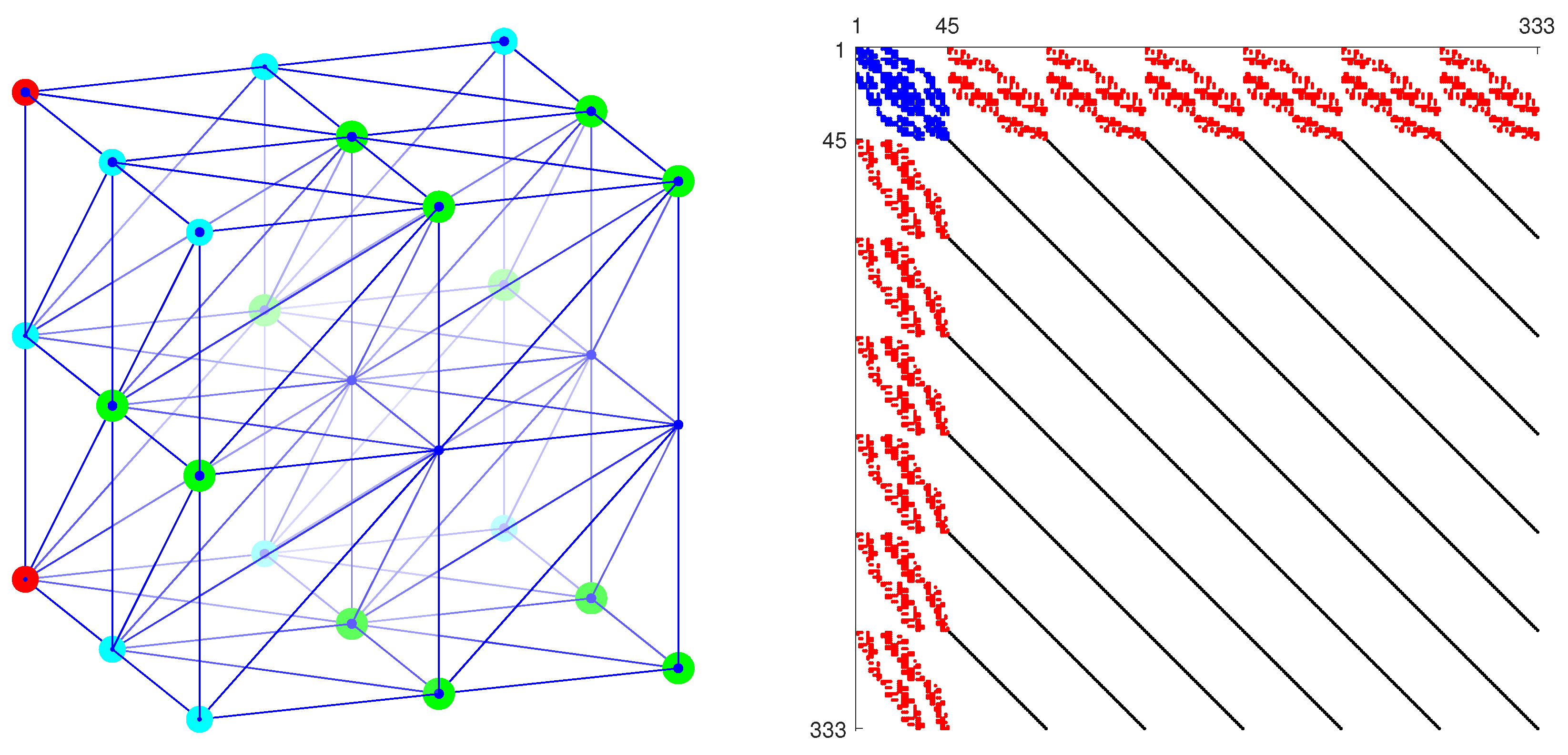
• Two nodes are constrained in all three directions (indicated by red circles);
• Nine nodes are constrained in two directions (indicated by violet circles);
• Twelve nodes are constrained in one direction (indicated by green circles).

Together, they fix$2·3+9·2+12=36$components of the displacement vector. Therefore, the remaining$27·3-36=45$components of the displacement vector are searched together with$6·48=288$components of internal variables. Thus, the total size of the minimization problem in Equation (14) is equal to$45+288=333$.

Figure 1 (right) illustrates the corresponding Hessian sparsity pattern. The blue dots mark the nonzero entries of the square block related only to 45 displacement degrees of freedom, and the black dots form the lines of the nonzero entries in the square block related to internal variables only. The clusters of red dots denote the nonzero entries in the remaining two blocks; they indicate the coupling between the components of displacement and the internal variables.

For the minimization, we employ the trust region optimization method available in the MATLAB Optimization Toolbox. As demonstrated in [37], providing additional information in terms of the gradients and sparsity pattern of the Hessian matrix (i.e., positions (indices) of its nonzero entries) substantially accelerates the computations. Numerical determination of the gradients (with a difference scheme) needed in optimization requires relatively little additional effort, and thus, it can be particularly advantageous for the development and refinement of constitutive laws of new materials with complex microstructural processes, where the quest for a particular form of the constitutive law is the principal endeavor.

The finite element discretization directly affects the construction of the gradient and the sparsity pattern. Whereas internal variables are approximated in $P^0\left(\mathfrak{T}\right)$, there are hence no inter-elemental links, and $P^1\left(\mathfrak{T}\right)$ is used for components of the displacement field. Thus, a nodal perturbation directly modifies the computations for all adjacent tetrahedral elements. The vectorized evaluation of the gradient components was developed and described in detail in [11], and the full vectorization of the constitutive core implemented in this work are thus vital for the efficient integration of gradient-evaluating minimization methods.

4. Computational Examples

In this section, we present three computational simulations to demonstrate the capabilities of our computational tool. All computations were performed on a MacBook Air (M1 processor, 2020) with 16 GB of memory.

Table 1. Table of material parameters with their brief descriptions. A and M denote austenite and martensite, respectively.

Parameter	Value	Unit	Brief Description
K	150	GPa	Bulk modulus common to both phases.
$G^{\mathrm{A}},G^{\mathrm{M}}$	$18,11$	GPa	Shear moduli of A and M.
k	$0.062$	1	Maximum transformation strain in tension.
a	$0.95$	1	Asymmetry parameter.
As, Af Ms, Mf Teq	5,7 −5, −8 0	$\}$${}^{°}$C	$\}$ Temperature parameters related to the direct phase transformation between A and M.
${\sigma }^{\mathrm{reo}}$	100	MPa	Reorientation stress of M at 25 ${}^{°}$C.
$\mathsf{\Delta }{s}^{\mathrm{AM}}$	$0.36$	MPa/${}^{°}$C	Difference between specific entropies of M and A.
$c^{\mathrm{reg}}$	$0.06$	MPa	Parameter of regularization function r in [22].
$E^{\mathrm{hrd}}$	$0.6$	MPa	Parameter of reorientation-hardening function.

presents the values of the material parameters inspired by [38] and used in all computational examples in this section, where $\mathbb{D}$ is set to the fourth-order identity tensor in Equation (6).

The first two subsections validate the constitutive law in simple loading modes common for shape memory alloys. The simulations were performed on a simple computational cubic domain of a unit length of 1 cm, which was subjected to variations in temperature, and mechanical loading was applied on the top face. The displacements on the bottom and two side faces were fixed in directions parallel with the corresponding face normals (to avoid rigid body motion). The domain was divided into eight equal cuboids, each consisting of six equal tetrahedral elements. Due to the invoked uniform loading modes, the results within all the elements were equal within the numerical error.

The example in the last subsection deals with a more complex (inhomogenous) mechanical state of the material body to demonstrate the capabilities of the complete computational tool.

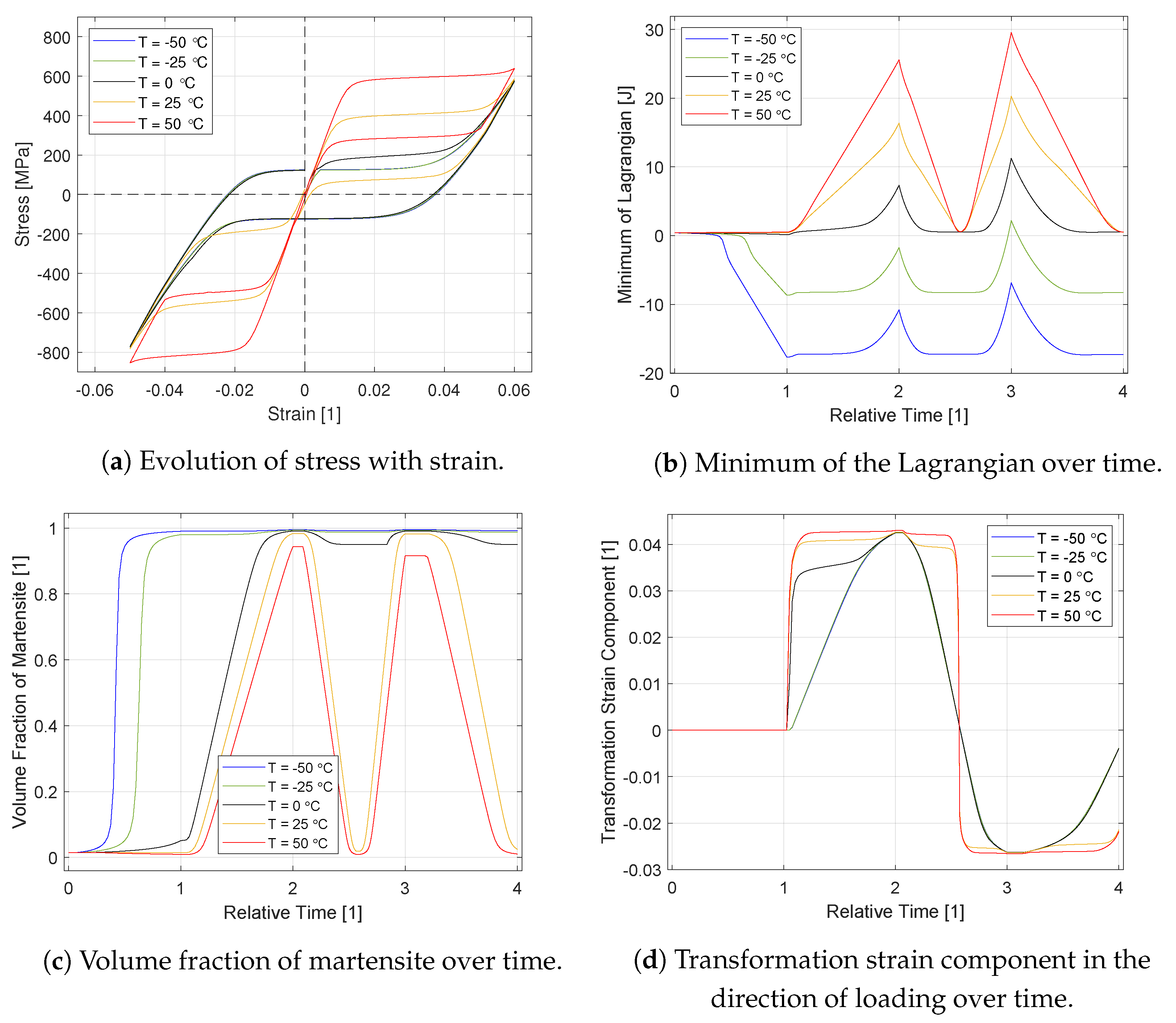
4.1. Example 1: Uniaxial Tension–Compression Tests at Different Temperatures

First, we present the results of uniaxial tests performed via Dirichlet-type boundary conditions. Figure 2 presents the results of the simulation of the uniaxial tension–compression tests at five different constant temperatures, namely $-50{}^{°}\mathrm{C}$, $-25{}^{°}\mathrm{C}$, $0{}^{°}\mathrm{C}$, $25{}^{°}\mathrm{C}$, and $50{}^{°}\mathrm{C}$. Each simulation was divided into four steps (distinguished by “relative time” in the plots): (1) the temperature of the body was changed from room temperature ($25{}^{°}\mathrm{C}$, or above $A_{\mathrm{f}}$) to the desired one under no change in displacement, (2) the corresponding displacement of nodes on the top face of the cube was increased up to 0.06, (3) the displacement was decreased to −0.05, and (4) the displacement was again increased to zero. Except for the first step, the temperature was held constant (and uniform).

The results in Figure 2a show the evolution typical for the shape memory alloys: a pseudoplastic type of response at low temperatures ($-50{}^{°}\mathrm{C}$ and $-25{}^{°}\mathrm{C}$, with coinciding graphs), superelastic type of response at high temperatures ($25{}^{°}\mathrm{C}$ and $50{}^{°}\mathrm{C}$), and an intermediate response in between ($0{}^{°}\mathrm{C}$). This interpretation is backed by the plot of the evolution of the volume fraction of martensite within the steps in Figure 2c. For the two lowest temperatures, the almost full martensitic state was reached after cooling (end of step 1, i.e., relative time equals 1), whereas for the rest, transformation to martensite was induced after loading was applied (step 2). Since $0{}^{°}\mathrm{C}$ was below the temperature needed for the initiation of the reverse transformation to austenite, most of the martensite remained stable even during the unloading stages of the test (in steps 3 and 4). This contrasted with the two higher temperatures, where austenite was recovered during unloading. Figure 2d shows the evolution of the relevant component of the transformation strain tensor, where the difference between the minimum and maximum reached values imposed via Equation (5), and Equation (6) resulted in the pronounced tension–compression asymmetry in Figure 2a. For instance, the critical stress for the transition to martensite was higher, and the plateau strain was lower in compression compared with the tension in the superelastic regime. The complex processes linked with energy storage and dissipation gave rise to the patterns of $J_{\mathrm{SMA}}^{\tau }$-functional minimum in Figure 2b, which are entirely distinct from the quadratic ones known in Hookean elasticity.

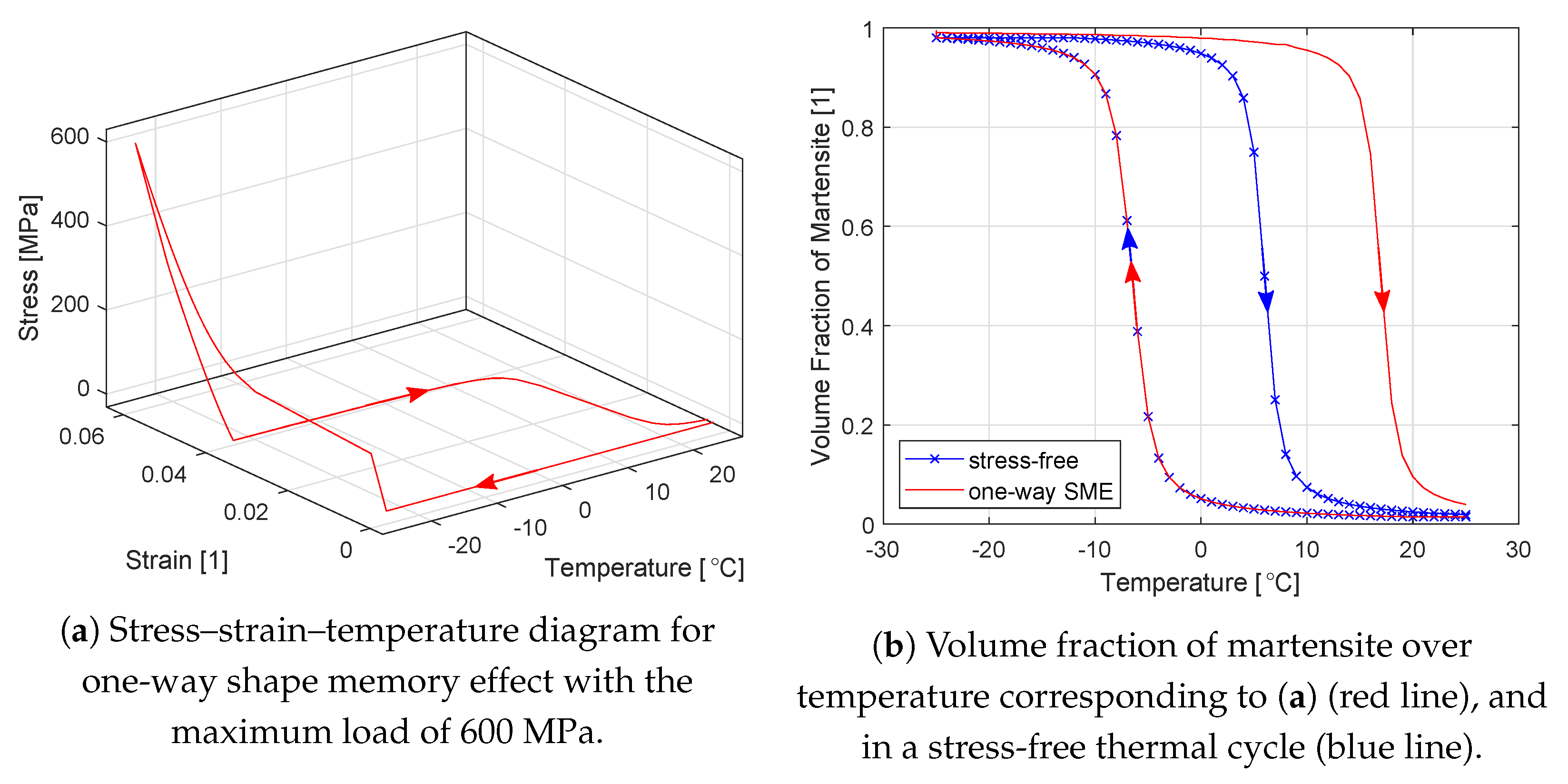
4.2. Example 2: One-Way Shape Memory Effect and Martensite Stabilization Effect

To demonstrate the ability to employ the Neumann type of boundary condition, we simulated the so-called one-way shape memory effect, an important phenomenon utilized in applications [27]. The cube was cooled down to $-25{}^{°}\mathrm{C}$ first and then loaded to 600 MPa (via imposing the Neumann condition on the top cube face), unloaded via complete removal of the stress, and finally heated to room temperature ($25{}^{°}\mathrm{C}$). The results in terms of the stress–strain–temperature space and the evolution of the volume fraction of martensite with the temperature are depicted in Figure 3a,b, respectively. After unloading (at $-25{}^{°}\mathrm{C}$), the material remained martensitic, with the strain reaching almost $4\%$. Only when it was heated enough did it transform back to austenite and return to the original configuration (shape). Hence, the strain was released, as observed in the experiments in [27].

For comparison, Figure 3b also includes the situation, in which the interlude of loading and unloading was omitted (i.e., the material was just cooled down and heated up without straining). It is worth noting that the temperature interval for the reverse transition in the one-way shape memory effect (approximately between $10{}^{°}\mathrm{C}$ and $20{}^{°}\mathrm{C}$) significantly shifted upward with respect to the stress-free thermal cycle ($0{}^{°}\mathrm{C}$ and $10{}^{°}\mathrm{C}$, cf. $M_{\mathrm{s}}$ and $M_{\mathrm{f}}$ in Table 1). This temperature shift was due to the so-called “martensite (mechanical) stabilization”, and it has been experimentally well-documented [39,40,41]. In the constitutive model, this is due to the particular form of the dissipation function in Equation (8), which also recognizes the contribution linked with the reverse transformation of reoriented martensite.

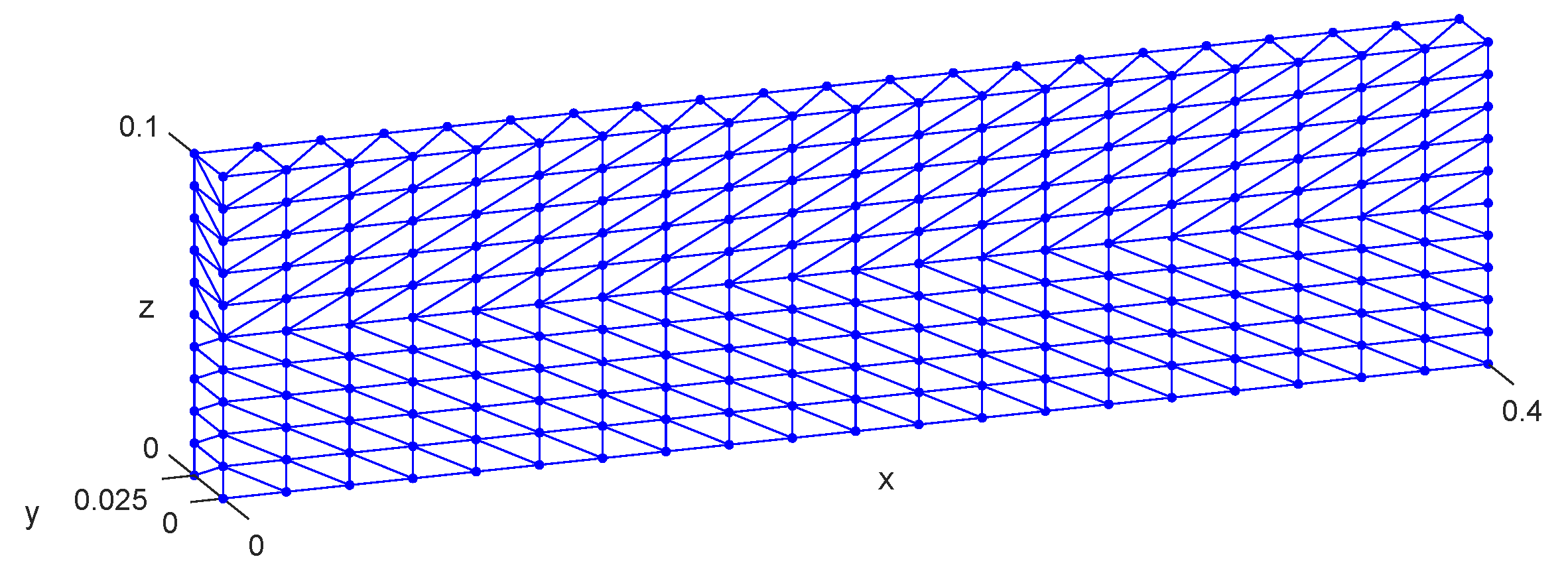
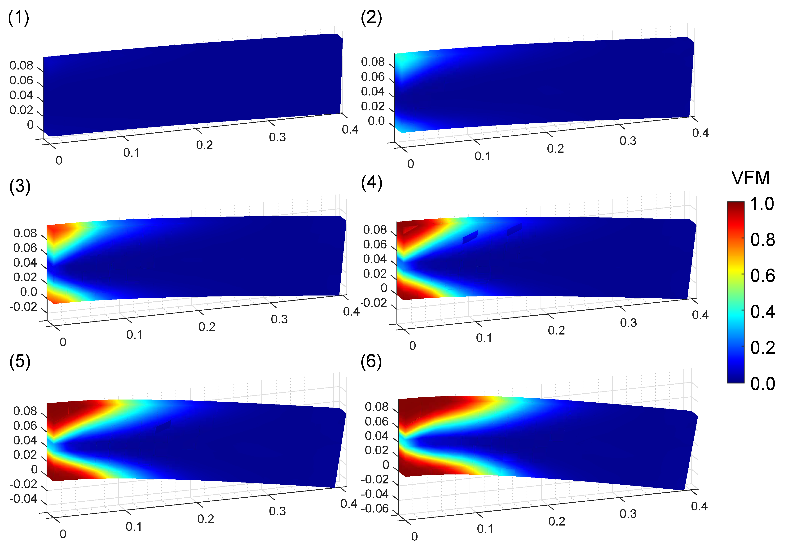
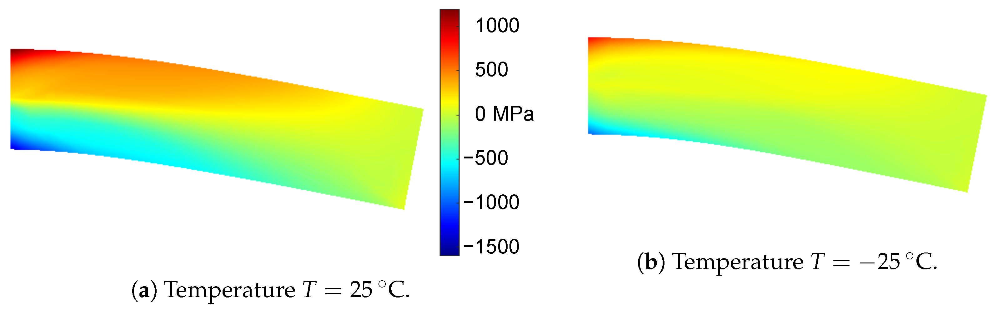
4.3. Example 3: Bending of a Shape Memory Alloy Beam

The performance of the complete FEM computational tool is now demonstrated in the example of the bending of a beam. Beams manufactured from shape memory alloys have been intensively investigated due to their superb actuation and energy harvesting capabilities [42,43,44]. Although analytical models can be very useful for quick concept validation and preliminary design studies [45,46,47], full-scale FEM simulations are often indispensable in detailed studies [42,44,48,49], since they are not constrained by assumptions on a particular geometry, material response, boundary conditions, etc. The simulated problem mimics a simple beam with a rectangular cross-section (with its width being half of the height) loaded at both ends and supported in the middle so that bending is invoked. Thanks to the expected structural symmetry of the situation with respect to two (out of three) symmetry planes of the beam, it was enough to model only one-fourth of the structure and hence fix the displacement of nodes adjacent to those planes of symmetry in a direction normal to the planes. The particular geometric model of the symmetry segment (length of 0.4 cm, height of 0.1 cm, and width of 0.025 cm) together with applied triangulation is depicted in Figure 4. The structured mesh with $20\times 1\times 10$ identical small cuboids each containing 6 tetrahedral elements was used to capture primarily the details in the x-z symmetry plane. Nodes on the plane $x=0\mathrm{cm}$ and $y=0.025\mathrm{cm}$ were constrained according to the symmetry requirements, nodes satisfying $x=0\mathrm{cm}$ and $z=0\mathrm{cm}$ were also constrained in z displacement (avoiding rigid body motion), and nodes satisfying $x=0.4\mathrm{cm}$ and $z=0\mathrm{cm}$ (“bottom end edge”) were linearly prescribed uniform displacement in a direction z so that they reached position $z=-0.06\mathrm{cm}$ in 6 increments. A uniform temperature of $25{}^{°}$C was considered during the whole simulation, and hence superelastic behavior was induced. Let us remind the reader that the current work adopted small strain and isothermality assumptions; a discussion of the influence of such premises on the results of computational simulations of shape memory beams can be found in [49].

The deformed configurations overlaid with contour plots showing the distribution of the volume fraction of martensite in each computational increment are shown in Figure 5. A continuous transformation was documented, starting from both the upper and lower sides of the beam and penetrating toward the central part containing the neutral plane. Let us note that validation of the SMA model via comparison with the experimentally determined distribution of phases has been performed recently [24,50].

Figure 6a shows the distribution of the diagonal component of the stress tensor in the x direction in the reference configuration in the last increment, (i.e., corresponding to Equation (6) in Figure 5). Due to the tension-compression asymmetry, its maximum tension was approximately 2/3 of the absolute maximum in compression, and the neutral plane shifted toward the compressed part of the material (cf. analytical computations in [46,51]). For comparison, the same computational simulation was performed at $-25{}^{°}\mathrm{C}$ (i.e., in the pseudoplastic regime of the material), and the distribution of the diagonal component of the stress tensor in the x direction is shown in Figure 6b. Both plots use the same color coding, which allows for direct comparison of the numerical values. Clearly, thanks to the lower net stiffness of martensite (which was reoriented during loading), the stress maxima in this were lower than in the superelastic case in Figure 6a. Such strong temperature dependence of the structural stiffness is employed in many applications [52].

5. Conclusions and Future Outlook

This work presents a successful implementation of the incremental energy minimization approach for rate-independent dissipative solids within a finite element framework. A model of shape memory alloys rigorously formulated in [23] served as a benchmark example of such a type of constitutive law. It features a strongly coupled, rate-independent dissipation function. The solution of an evolutionary boundary value problem of a solid body is constructed as a sequence of solutions of adjacent time-incremental boundary value problems in the spirit of the energetic solution concept for rate-independent materials [9]. Each of these fixed-time problems is considered to be a genuine minimization task (Equation (1)) discretized in space via the finite element method and resolved by conventional optimization tools. In this respect, the chosen monolithic approach represents a consistent alternative to the staggering minimization strategy employed in [23] and follows a thus far unexplored pathway offered by the energetic solution concept.

The vectorized implementation into MATLAB also presents the first step in a long-term activity focused on building a lightweight FEM-based computational tool tailored for rapid development, preliminary testing, and validation of new constitutive laws of dissipative materials with complex microstructural processes. Here, the motivation comes from material science and engineering, where the rapid progress in the manufacturing and characterization of new materials is often not fully exploited by the constitutive models. Among other factors, this is because the process of validation of new constitutive laws utilizing tailored implementation into computationally-aided engineering software suites is usually laborious and time-consuming. Employing a versatile FEM-based tool provides a viable alternative, especially in the initial stage of constitutive law development. Of course, when the form of the constitutive law is finally established, its tailored implementation in such suites (including developing its own constitutive subroutines) is inevitable for the resolution of more complex boundary problems (e.g., with geometry requiring adaptive remeshing or involving additional engineering phenomena as contacts). Following this idea, we adopted and substantially modified the vectorized code from [11] so that it could be used for both hyperelastic and rate-independent constitutive laws. The modifications include the introduction of internal variables and their history into the minimization process, adding a solution parameter (representing the temperature field), or handling the Neumann boundary conditions. The capabilities of the whole computational tool were tested on a problem of bending a shape memory alloy beam. The version presented in this work can be downloaded for free from a dedicated website.

The benefits of the applied approach come hand in hand with some limitations. The first one is related to the variational formulation. Although the class of constitutive models complying with Equation (2) is wide, a special mathematical and numerical treatment is needed for some types of models (e.g., the concept of bipotential [53] for materials with non-associative laws or the homogenization techniques for heterogeneous materials [54]) (see also the mathematical background in [9]). Second, the dimension of the minimization problem in the monolithic formulation is naturally higher than in the case when the problem is split in the nested formulation, which poses a challenge for computational resources. Third, applying universal minimization methods is often less efficient than employing customized algorithms and may lead to prohibitive computational time consumption for more complex evolutionary boundary problems. Whereas the first issue may require completely new numerical development, relatively milder modifications such as parallelization or algorithms of non-smooth optimization can help to at least partially remove a burden from the other two constraints.

Hence, one direction of planned future refinements of the numerical implementation resides in improving the computational speed. The time needed for the computation of gradient inputs to the optimization routines could be reduced, such as by including the methods of automatic differentiation (cf. [55]). Alternatively, one can even abandon the intrinsic MATLAB optimization tools and employ some progressive optimization methods tailored to the inherent structure of the rate-independent constitutive laws as, for example, fast iterative shrinkage-thresholding algorithms adapted for non-smooth functions [56]. Reformulation of the models within the finite strain (large deformation) theory poses another challenge, both from the modeling and from the implementation (vectorization) points of view. Inspiring attempts involving these aspects have been carried out (e.g., in [13,48,57]).

References

1. Halphen, B.; Nguyen, Q.S. Sur les matériaux standard généralisés. J. Mec. 1975, 14, 39–63. [Google Scholar]
2. Ziegler, H. An Introduction to Thermodynamics, 1st ed.; North-Holland Series in Applied Mathematics and Mechanics; North-Holland: Amsterdam, The Netherlands, 1983. [Google Scholar]
3. Germain, P.; Nguyen, Q.S.; Suquet, P. Continuum Thermodynamics. J. Appl. Mech. 1983, 50, 1010–1020. [Google Scholar] [CrossRef]
4. Houlsby, G.T.; Puzrin, A.M. A thermomechanical framework for constitutive models for rate-independent dissipative materials. Int. J. Plast. 2000, 16, 1017–1047. [Google Scholar] [CrossRef]
5. Hackl, K.; Fischer, F.D. On the relation between the principle of maximum dissipation and inelastic evolution given by dissipation potentials. Proc. R. Soc. Lond. Ser. A 2008, 464, 117–132. [Google Scholar] [CrossRef]
6. Petryk, H. Incremental energy minimization in dissipative solids. CR Mec. 2003, 331, 469–474. [Google Scholar] [CrossRef]
7. Miehe, C. Strain-driven homogenization of inelastic microstructures and composites based on an incremental variational formulation. Internat. J. Numer. Methods Engrg. 2002, 55, 1285–1322. [Google Scholar] [CrossRef]
8. Miehe, C. A multi-field incremental variational framework for gradient-extended standard dissipative solids. J. Mech. Phys. Solids 2011, 59, 898–923. [Google Scholar] [CrossRef]
9. Mielke, A.; Roubíček, T. Rate-Independent Systems: Theory and Application; Applied Mathematical Sciences; Springer: New York, NY, USA, 2015. [Google Scholar]
10. Owen, D.R.; Williams, W.O. On the concept of rate-independence. Quart. Appl. Math. 1968, 26, 321–329. [Google Scholar] [CrossRef] [Green Version]
11. Moskovka, A.; Valdman, J. Fast MATLAB evaluation of nonlinear energies using FEM in 2D and 3D: Nodal elements. Appl. Math. Comput. 2022, 424, 127048. [Google Scholar] [CrossRef]
12. Scalet, G.; Auricchio, F. Computational Methods for Elastoplasticity: An Overview of Conventional and Less-Conventional Approaches. Arch. Computat. Methods Eng. 2018, 25, 545–589. [Google Scholar] [CrossRef]
13. Stupkiewicz, S.; Petryk, H. A robust model of pseudoelasticity in shape memory alloys. Int. J. Numer. Methods Eng. 2013, 93, 747–769. [Google Scholar] [CrossRef]
14. Artioli, E.; Bisegna, P. An incremental energy minimization state update algorithm for 3D phenomenological internal-variable SMA constitutive models based on isotropic flow potentials. Int. J. Numer. Methods Eng. 2016, 105, 197–220. [Google Scholar] [CrossRef]
15. Scalet, G.; Peigney, M. A robust and efficient radial return algorithm based on incremental energy minimization for the 3D Souza-Auricchio model for shape memory alloys. Eur. J. Mech. A Solids 2017, 61, 364–382. [Google Scholar] [CrossRef] [Green Version]
16. Egner, H.; Skoczen, B.; Rys, M. Constitutive and numerical modeling of coupled dissipative phenomena in 316L stainless steel at cryogenic temperatures. Int. J. Plast. 2015, 64, 113–133. [Google Scholar] [CrossRef]
17. Peigney, M.; Scalet, G.; Auricchio, F. A time-integration algorithm for a 3D constitutive model for SMAs including permanent inelasticity and degradation effects. Int. J. Numer. Methods Eng. 2018, 115, 1053–1082. [Google Scholar] [CrossRef] [Green Version]
18. Einav, I.; Houlsby, G.T.; Nguyen, G.D. Coupled damage and plasticity models derived from energy and dissipation potentials. Int. J. Solids Struct. 2007, 44, 2487–2508. [Google Scholar] [CrossRef] [Green Version]
19. Rahman, T.; Valdman, J. Fast MATLAB assembly of FEM matrices in 2D and 3D: Nodal elements. Appl. Math. Comput. 2013, 219, 7151–7158. [Google Scholar] [CrossRef]
20. Anjam, I.; Valdman, J. Fast MATLAB assembly of FEM matrices in 2D and 3D: Edge elements. Appl. Math. Comput. 2015, 267, 252–263. [Google Scholar] [CrossRef] [Green Version]
21. Cimrman, R.; Lukeš, V.; Rohan, E. Multiscale finite element calculations in Python using SfePy. Adv. Comput. Math. 2019, 45, 1897–1921. [Google Scholar] [CrossRef] [Green Version]
22. Sedlák, P.; Frost, M.; Benešová, B.; Šittner, P.; Ben Zineb, T. Thermomechanical model for NiTi-based shape memory alloys including R-phase and material anisotropy under multi-axial loadings. Int. J. Plast. 2012, 39, 132–151. [Google Scholar] [CrossRef]
23. Frost, M.; Benešová, B.; Sedlák, P. A microscopically motivated constitutive model for shape memory alloys: Formulation, analysis and computations. Math. Mech. Solids 2016, 21, 358–382. [Google Scholar] [CrossRef]
24. Frost, M.; Sedlák, P.; Kadeřávek, L.; Heller, L.; Šittner, P. Modeling of mechanical response of NiTi shape memory alloy subjected to combined thermal and non-proportional mechanical loading: A case study on helical spring actuator. J. Intel. Mat. Syst. Str. 2016, 27, 1927–1938. [Google Scholar] [CrossRef]
25. Frost, M.; Benešová, B.; Seiner, H.; Kružík, M.; Šittner, P.; Sedlák, P. Thermomechanical model for NiTi-based shape memory alloys covering macroscopic localization of martensitic transformation. Int. J. Solids Struct. 2021, 221, 117–129. [Google Scholar] [CrossRef]
26. Benešová, B.; Frost, M.; Kadeřávek, L.; Roubíček, T.; Sedlák, P. An experimentallly-fitted thermodynamical constitutive model for polycrystalline shape memory alloys. Disc. Cont. Dynam. Syst. S 2021, 14, 3925–3952. [Google Scholar] [CrossRef]
27. Otsuka, K.; Wayman, C.M. Shape Memory Materials; Cambridge University Press: Cambridge, UK, 1998. [Google Scholar]
28. Elkhal Letaief, W.; Hassine, T.; Gamaoun, F.; Sarraj, R.; Ben Kahla, N. Coupled diffusion-mechanical model of NiTi alloys accounting for hydrogen diffusion and ageing. Int. J. Appl. Mech. 2020, 12, 2050039. [Google Scholar] [CrossRef]
29. Wang, L.; Feng, P.; Xing, X.; Wu, Y.; Liu, Z. A one-dimensional constitutive model for NiTi shape memory alloys considering inelastic strains caused by the R-phase transformation. J. Alloy. Compd. 2021, 868, 159192. [Google Scholar] [CrossRef]
30. Wang, L.; Feng, P.; Wu, Y.; Liu, Z. A Temperature-Dependent Model of Shape Memory Alloys Considering Tensile-Compressive Asymmetry and the Ratcheting Effect. Materials 2020, 13, 3116. [Google Scholar] [CrossRef]
31. Zhu, X.; Chu, L.; Dui, G. Constitutive Modeling of Porous Shape Memory Alloys Using Gurson–Tvergaard–Needleman Model Under Isothermal Conditions. Int. J. Appl. Mech. 2020, 12, 2050038. [Google Scholar] [CrossRef]
32. Adeodato, A.; Vignoli, L.L.; Paiva, A.; Monteiro, L.L.; Pacheco, P.M.; Savi, M.A. A Shape Memory Alloy Constitutive Model with Polynomial Phase Transformation Kinetics. Shap. Mem. Superelasticity 2022. [Google Scholar] [CrossRef]
33. Jiang, D.; Xiao, Y. Modelling on grain size dependent thermomechanical response of superelastic NiTi shape memory alloy. Int. J. Solids Struct. 2021, 210, 170–182. [Google Scholar] [CrossRef]
34. Auricchio, F.; Petrini, L. Improvements and algorithmical considerations on a recent three-dimensional model describing stress-induced solid phase transformations. Int. J. Numer. Methods Eng. 2002, 55, 1255–1284. [Google Scholar] [CrossRef]
35. Ciarlet, P.G. The Finite Element Method for Elliptic Problems; Classics in Applied Mathematics; SIAM: Phiadelphia, PA, USA, 2002. [Google Scholar]
36. Alberty, J.; Carstensen, C.; Funken, S.A.; Klose, R. Matlab Implementation of the Finite Element Method in Elasticity. Computing 2002, 69, 239–263. [Google Scholar] [CrossRef]
37. Matonoha, C.; Moskovka, A.; Valdman, J. Minimization of p-Laplacian via the Finite Element Method in MATLAB. In International Conference on Large-Scale Scientific Computing, (LSSC 2021); Lecture Notes in Computer Science; Lirkov, I., Margenov, S., Eds.; Springer: Berlin/Heidelberg, Germany, 2022; Volume 13127, pp. 533–540. [Google Scholar]
38. Šittner, P.; Heller, L.; Pilch, J.; Sedlák, P.; Frost, M.; Chemisky, Y.; Duval, A.; Piotrowski, B.; Ben Zineb, T.; Patoor, E.; et al. Roundrobin SMA modeling. In ESOMAT 2009—The 8th European Symposium on Martensitic Transformations; Šittner, P., Heller, L., Paidar, V., Eds.; EDP Sciences: Ulis, France, 2009; p. 08001. [Google Scholar]
39. Piao, M.; Otsuka, K.; Miyazaki, S.; Horikawa, H. Mechanism of the As temperature increase by pre-deformation in thermoelastic alloys. Mater. Trans. JIM 1993, 34, 919–929. [Google Scholar] [CrossRef] [Green Version]
40. Liu, Y.; Favier, D. Stabilisation of martensite due to shear deformation via variant reorientation in polycrystalline NiTi. Acta Mater. 2000, 48, 3489–3499. [Google Scholar] [CrossRef]
41. Belyaev, S.; Resnina, N.; Iaparova, E.; Ivanova, A.; Rakhimov, T.; Andreev, V. Influence of chemical composition of NiTi alloy on the martensitestabilization effect. J. Alloy. Compd. 2019, 787, 1365–1371. [Google Scholar] [CrossRef]
42. Rao, Z.; Wang, X.; Leng, J.; Yan, Z.; Yan, X. Design methodology of the Ni50Ti50 shape memory alloy beam actuator: Heat treatment, training and numerical Simulation. Mater. Des. 2022, 217, 110615. [Google Scholar] [CrossRef]
43. Viet, N.V.; Zaki, W.; Umer, R. Analytical investigation of an energy harvesting shape memory alloy piezoelectric beam. Arch. Appl. Mech. 2020, 90, 2715–2738. [Google Scholar] [CrossRef]
44. Seigner, L.; Tshikwand, G.K.; Wendler, F.; Kohl, M. Bi-Directional Origami-Inspired SMA Folding Microactuator. Actuators 2021, 10, 181. [Google Scholar] [CrossRef]
45. Eshghinejad, A.; Elahinia, M. Exact solution for bending of shape memory alloy beams. Mech. Adv. Mater. Struc. 2015, 22, 829–838. [Google Scholar] [CrossRef]
46. Viet, N.V.; Zaki, W.; Moumni, Z. A model for shape memory alloy beams accounting for tensile compressive asymmetry. J. Intell. Mater. Syst. Struct. 2019, 30, 2697–2715. [Google Scholar] [CrossRef]
47. Radi, E. Analytical modeling of the shape memory effect in SMA beams with rectangular cross section under reversed pure bending. J. Intell. Mater. Syst. Struct. 2021, 32, 2214–2230. [Google Scholar] [CrossRef]
48. Sielenkämper, M.; Wulfinghoff, S. A thermomechanical finite strain shape memory alloy model and its application to bistable actuators. Acta Mech. 2022, 3059–3094, 233. [Google Scholar] [CrossRef]
49. Kundu, A.; Banerjee, A. Coupled thermomechanical modelling of shape memory alloy structures undergoing large deformation. Int. J. Mech. Sci. 2022, 220, 107102. [Google Scholar] [CrossRef]
50. Frost, M.; Sedlák, P.; Heller, L.; Kadeřávek, L.; Šittner, P. Experimental and computational study on phase transformations in superelastic NiTi snake-like spring. Smart Mater. Struct. 2018, 27, 095005. [Google Scholar] [CrossRef]
51. Ostadrahimi, A.; Taheri-Behrooz, F.; Choi, E. Effect of Tension-Compression Asymmetry Response on the Bending of Prismatic Martensitic SMA Beams: Analytical and Experimental Study. Materials 2021, 14, 5415. [Google Scholar] [CrossRef]
52. Mohd Jani, J.; Leary, M.; Subic, A. Designing shape memory alloy linear actuators: A review. J. Intell. Mater. Syst. Struct. 2017, 28, 1699–1718. [Google Scholar] [CrossRef]
53. De Saxcé, G.; Feng, Z.Q. New inequality and functional for contact with friction: The implicit standard material approach. J. Struct. Mech. 1991, 19, 301–325. [Google Scholar] [CrossRef]
54. Lahellec, N.; Suquet, P. On the effective behavior of nonlinear inelastic composites: I. Incremental variational principles. J. Mech. Phys. Solids 2007, 55, 1932–1963. [Google Scholar] [CrossRef] [Green Version]
55. Blühdorn, J.; Gauger, N.R.; Kabel, M. AutoMat: Automatic differentiation for generalized standard materials on GPUs. Comput. Mech. 2022, 69, 589–613. [Google Scholar] [CrossRef]
56. Beck, A.; Teboulle, M. A Fast Iterative Shrinkage-Thresholding Algorithm for Linear Inverse Problems. SIAM J. Imaging Sci. 2009, 2, 183–202. [Google Scholar] [CrossRef] [Green Version]
57. Drozdenko, D.; Knapek, M.; Kružík, M.; Máthis, K.; Švadlenka, K.; Valdman, J. Elastoplastic Deformations of Layered Structures. Milan J. Math. 2022. [Google Scholar] [CrossRef]
Figure 1. An illustrative triangulation of a cubic domain (see Examples 1 and 2 in Section 4) with nodes with restricted displacement marked by circles (left) and the corresponding sparsity pattern of the Hessian matrix (right). See text for details.
Mathematics 10 04412 g001
Figure 2. Uniaxial tests at five different temperatures (Example 1).
Mathematics 10 04412 g002
Figure 3. One-way shape memory effect (Example 2).
Mathematics 10 04412 g003
Figure 4. Finite element model of a shape memory alloy beam with the initial mesh layout (Example 3).
Mathematics 10 04412 g004
Figure 5. Simulation of bending a beam at 25 ° C. The color maps show the distribution of volume fraction of martensite (VFM) at six loading increments; the colorbar applies to all six plots (Example 3).
Mathematics 10 04412 g005
Figure 6. Deformed configuration with a contour plot of the normal stress component parallel to the x axis (within the reference configuration). The color bar applies to both plots (Example 3).
Mathematics 10 04412 g006