Improved Fractional-Order Extended State Observer-Based Hypersonic Vehicle Active Disturbance Rejection Control

Abstract

In this work, a novel fractional-order extended state observer (FOESO)-based linear active disturbance rejection control (LADRC) method is firstly proposed for a hypersonic vehicle (HV) to address the measurement noise problem. The uncertainty and external disturbance of an HV was discussed and addressed by the active disturbance rejection control and many different control methods in recent decades. However, the research of an HV with measurement noise is insufficient. For the LADRC, the anti-noise ability is highly dependent on the bandwidth of the extended state observer (ESO). Meanwhile, the control performance of the LADRC is relevant to the bandwidth. The FOESO is presented, aiming to address the tradeoff of the control performance or noise suppression. The FOESO-based LADRC (FOESO-LADRC) introduces fractional calculus. It can enhance the anti-noise ability with little influence on the control performance. The simulation results show that the FOESO-LADRC has a significant improvement in the noise suppression. In addition, compared with the LADRC, it obtains a better solution to address the tradeoff between the bandwidth and noise impact.

1. Introduction

A hypersonic vehicle (HV) is a class of advanced aircraft. It can fly at an extremely high speed with a considerable long range. However, it has the disadvantages of a large flight envelope, strong coupling, strong nonlinearity and aerodynamic uncertainty, which enlarge the uncertainty of the control system [1].

The problem of the high-performance control of an HV with an internal and external disturbance was investigated worldwide. There are many control approaches that were studied, such as the robust control [2,3], backstepping control [4,5], model predict control [6], sliding model control [7,8] and intelligent control.

The active disturbance rejection control (ADRC), as the inheritance and development of the traditional PID control, is an error feedback-based control method which has a low requirement of the plant information. Compared with the PID, the ADRC has a better robustness to both the internal and external disturbance. The ADRC is firstly proposed by Han [9]. It consists of three parts: the tracking differentiator (TD), state feedback controller (SFC) and extended state observer (ESO). Gao et al. develop the ADRC to the LADRC [10]. It establishes the SFC and linear ESO (LESO) according to the control bandwidth and LESO bandwidth, which shows the explicit meaning of the control parameters. The capabilities of the SFC and LESO are crucial to the control performance of the LADRC. Therefore, many studies were carried out to improve the SFC and LESO. For systems with an unknown upper bound of uncertainty, a positive increasing function associated with the observer objective is employed to guarantee the estimation error converges in finite time [11]. Razmjooei et al. combine the disturbance observer and nonlinear feedback control for electro-hydraulic position tracking [12,13]. The well-designed observer and nonlinear feedback controller can make the estimation error converge in finite time. Zhao et al. propose an ESO-based backstepping control algorithm combining the ADRC and a backstepping algorithm [14]. It enables the system to converge precisely and quickly in a fixed time. Gao et al. combine the ADRC and fractional-order PID control method [15]. Compared with the traditional ADRC, the proposed method shows a better control performance with an actuator efficiency reduction. The ESO estimates and compensates the total disturbance. In recent years, plenty of studies focused on the improvement in the ESO. Sun et al. present a novel ADRC combining the ESO and conditional disturbance negation method [16]. It divides disturbances into two categories, the detriment disturbance and benefit disturbance, and only compensate the detriment disturbance. Wei et al. use a phase-leading method to alter the frequency-domain characteristics of the ESO [17]. The study shows that a phase-leading ESO-based ADRC is superior to a traditional ADRC in both the response and disturbance rejection performance. Gao et al. replace the PID controller of an ADRC with an FOPID controller. It introduces two additional fractional calculus operators. With well-tuned fractional-order parameters, the FOPID shows a better robustness and performance than the PID [6]. For a fractional-order system, numerous studies [18,19,20,21] were conducted to establish a fractional-order ESO (FOESO) to make the ADRC more suitable for the system. For an integral-order system, Chen et al. implement the FOESO by considering the nominal system as a fractional integral series. The simulation results illustrate that the proposed FOESO has a better dynamic performance and anti-noise ability. Nevertheless, the physical meaning of the total disturbance was changed while establishing the FOESO, because the additional model uncertainty is introduced to the FOESO.

The ADRC has great advantages to address the internal and external disturbance which has an obvious impact on the HV control system. Therefore, an HV with an ADRC was widely discussed in recent years [6,15,16,22,23]. For example, Piao et al. design two types of practical control schemes for the HV angle of attack [22]. One is applying a second-order ADRC to the second-order system, and the other combines the first-order ADRC with an inner loop pitch angular rate feedback control. Both of the ADRC schemes show a strong robustness to the HV unmodeled dynamic, parametric uncertainties and external disturbances. Tian et al. use feedback linearization and an equivalent input disturbance technique to disassemble the HV nonlinear system into several subsystems in a canonical form and design an ADRC, respectively [23]. It achieves a precise tracking performance with parametric perturbations and atmospheric disturbances.

In spite of the extensive and successful development of the HV with an ADRC, one problem remains: the measurement noise of the HV is rarely discussed. The actual HV is exposed to radiation and mechanical vibration in its working condition. It will cause an inevitable measurement noise [24]. In addition, the influence of the measurement noise is significantly different from the internal and external disturbance. Several studies were proposed to suppress the measurement noise via different control methods [24,25,26,27]. As for the LADRC, the measurement noise has an important influence. The increasing of the bandwidth will amplify the response of the measurement noise. It constrains the upper bound of the LESO bandwidth, which is crucial to the speed of response. A positive increasing function associated with the observer objectives is employed to improve the convergence time performance. The simulation results show that the proposed observer can compete with other leading strategies.

Motivated by the above considerations, an FOESO is proposed in this article to suppress noise with a non-significant sacrifice of the control performance. The fractional calculus is introduced to cooperate with the gain of the observer. It could provide a better solution while addressing the aforementioned tradeoff of the anti-noise ability and control performance.

The remainder of the paper is structured as follows. In Section 2, the nonlinear model and linearized model of the HV are given. In Section 3, an FOESO-LADRC scheme is proposed, and the stable condition is established. In Section 4, the simulation results demonstrate that the FOESO-LADRC obtains a better solution to address the tradeoff between the bandwidth and noise impact compared with the LADRC.

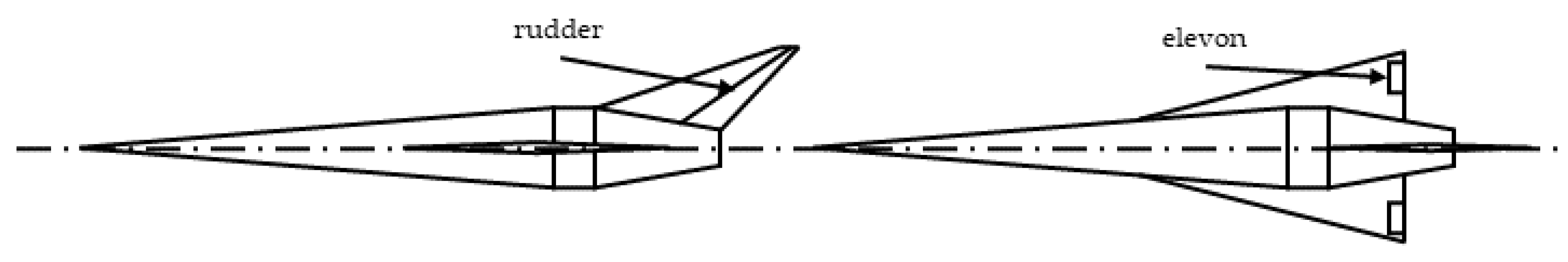
2. Dynamic Model of Hypersonic Vehicle

The hypersonic vehicle studied in this article is purposed based on the winged-cone model with detailed information published by NASA’s Langley Research Center in 1990 [28]. Considering the requirement of future studies, some appropriate modifications are made. The geometry size, mass and rotary inertia are shown in Figure 1 and

Table 1. Mass and Rotary Inertia of Hypersonic Vehicle.

Parameters	Value	Parameters	Value
Mass	1250 kg	Reference area	3.35 m2
Vehicle length	6.1 m	Rolling moment	156 kg·m2
Lateral-directional reference length	1.83 m	Yawing moment	1162 kg·m2
Longitudinal reference length	2.44 m	Pitching moment	1267 kg·m2
Distance from nose to the center of gravity	3.78 m

.

The following equation shows the six-degrees-of-freedom hypersonic vehicle nonlinear model.

$$\dot{x}=V\cos \theta \cos {\psi }_c$$

(1)

$$\dot{y}=V\sin \theta$$

(2)

$$\dot{z}=-V\cos \theta \sin {\psi }_c$$

(3)

$$\dot{V}=-\frac{D}{m}+\frac{g}{r}\left(x\cos {\psi }_c\cos \theta +\left(y+R\right)\sin \theta -z\sin {\psi }_c\cos \theta \right)$$

(4)

$$\dot{\theta }=\frac{L\cos {\gamma }_c-Z\sin {\gamma }_c}{mV\cos {\psi }_c}+\frac{g}{rV\cos {\psi }_c}\left(-x\cos {\psi }_c\sin \theta +\left(y+R\right)\cos \theta +z\sin {\psi }_c\sin \theta \right)$$

(5)

$${\dot{\psi }}_c=-\frac{L\sin {\gamma }_c+Z\cos {\gamma }_c}{mV}-\frac{g}{rV}\left(x\sin {\psi }_c+z\cos {\psi }_c\right)$$

(6)

$${\dot{\omega }}_x=\frac{\left(I_{yy}-I_{zz}\right)}{I_{xx}}{\omega }_y{\omega }_z+\frac{1}{I_{xx}}\left(l_A+l_{Tr}\right)$$

(7)

$${\dot{\omega }}_y=\frac{\left(I_{zz}-I_{xx}\right)}{I_{yy}}{\omega }_x{\omega }_z+\frac{1}{I_{yy}}\left(m_A+m_{Tr}\right)$$

(8)

$${\dot{\omega }}_z=\frac{\left(I_{xx}-I_{yy}\right)}{I_{zz}}{\omega }_x{\omega }_y+\frac{1}{I_{zz}}\left(n_A+n_{Tr}\right)$$

(9)

$$\dot{\alpha }={\omega }_z-{\omega }_x\cos \alpha \tan \beta +{\omega }_y\sin \alpha \tan \beta -\frac{1}{mV\cos \beta }\left(L+mg\cos \theta \cos {\gamma }_c\right)$$

(10)

$$\dot{\beta }={\omega }_x\sin \alpha +{\omega }_y\cos \alpha +\frac{1}{mV}\left(Z-mg\cos \theta \sin {\gamma }_c\right)$$

(11)

$$\begin{array}{l}{\dot{\gamma }}_{\mathrm{c}}={\omega }_x\frac{\cos \alpha }{\cos \beta }-{\omega }_y\frac{\sin \alpha }{\cos \beta }\\ +\frac{1}{mV}\left(L\left(\sin \theta \sin {\gamma }_c+\tan \beta \right)+Z\sin \theta \cos {\gamma }_c+mg\cos \theta \cos {\gamma }_c\tan \beta \right)\end{array}$$

(12)

where V represents the velocity. θ and Ψ_c denote the flight path angle and flight path azimuth angle, respectively. ω_x, ω_y and ω_z are the angular rates in the body coordinate system. α, β and γ_c are the attack angle, sideslip angle and speed roll angle, respectively. x, y and z denote the position in the inertial coordinate system. g represents gravitational acceleration. R denotes the radius of the earth. D, L and Z represent the drag force, lift force and side force. l, $m$ and n with different corner marker represent the roll, yaw and pitch moment. In addition, the corner marker A and Tr denote that the moment is generated by aerodynamic force or control force, respectively. I_xx, I_yy and $I_{zz}$ are the moments of inertia.

To design an ADRC controller, a linear decoupled system is necessary. Based on the nonlinear HV model, the linearized HV attitude model is established as follows:

Differentiate (10), (11) and (12). Define $F_a=\ddot{\alpha }$, $F_{\beta }=\ddot{\beta }$, $F_{{\gamma }_c}={\ddot{\gamma }}_c$. The second derivative of $\alpha$, $\beta$ and ${\gamma }_c$ can be expressed as:

$$\begin{array}{l}\ddot{\alpha }=\frac{\partial F_{\alpha }}{\partial \alpha }\alpha +\frac{\partial F_{\alpha }}{\partial \dot{\alpha }}\dot{\alpha }+\frac{n_{Tr}}{I_{zz}}+f_{\alpha }\\ \ddot{\beta }=\frac{\partial F_{\beta }}{\partial \beta }\beta +\frac{\partial F_{\beta }}{\partial \dot{\beta }}\dot{\beta }+\frac{m_{Tr}}{I_{yy}}+f_{\beta }\\ {\ddot{\gamma }}_c=\frac{\partial F_{{\gamma }_c}}{\partial {\gamma }_c}{\gamma }_c+\frac{\partial F_{{\gamma }_c}}{\partial {\dot{\gamma }}_c}{\dot{\gamma }}_c+\frac{l_{Tr}}{I_{xx}}+f_{{\gamma }_c}\end{array}$$

(13)

where $f_{\alpha }$, $f_{\beta }$ and $f_{{\gamma }_c}$ are ignored during linearization. Definition:

$$a_{0,{\gamma }_c}=\frac{\partial F_{{\gamma }_c}}{\partial {\dot{\gamma }}_c},a_{1,{\gamma }_c}=\frac{\partial F_{{\gamma }_c}}{\partial {\gamma }_c},a_{0,\beta }=\frac{\partial F_{\beta }}{\partial \dot{\beta }},a_{1,\beta }=\frac{\partial F_{\beta }}{\partial \beta },a_{0,\alpha }=\frac{\partial F_{\alpha }}{\partial \dot{\alpha }},a_{1,\alpha }=\frac{\partial F_{\alpha }}{\partial \alpha }$$

the state variables, input variables and output variables as follows:

$$x_T=\left(\begin{array}{c}{\gamma }_c\\ \beta \\ \alpha \\ {\dot{\gamma }}_c\\ \dot{\beta }\\ \dot{\alpha }\end{array}\right),u_T=\left(\begin{array}{c}{l}_{ac}\\ m_{ac}\\ n_{ac}\end{array}\right),y_T=\left(\begin{array}{c}{\gamma }_c\\ \beta \\ \alpha \end{array}\right)$$

(14)

x_T, u_T and $y_T$ denote the state variables, input variables and output variables. Therefore, the state-space equation of HV attitude control system can be expressed as follows:

$${\dot{x}}_T=A_T{x}_T+B_T{u}_T+f_T$$

(15)

where $A_T=\left(\begin{array}{cccccc}0& 0& 0& 1& 0& 0\\ 0& 0& 0& 0& 1& 0\\ 0& 0& 0& 0& 0& 1\\ -a_{1,{\gamma }_c}& 0& 0& -a_{0,{\gamma }_c}& 0& 0\\ 0& -a_{1,\beta }& 0& 0& -a_{0,\beta }& 0\\ 0& 0& -a_{1,\alpha }& 0& 0& -a_{0,\alpha }\end{array}\right)$, $B_T=\left(\begin{array}{ccc}0& 0& 0\\ 0& 0& 0\\ 0& 0& 0\\ \raisebox{1ex}{$1$}\!\left/ \!\raisebox{-1ex}{$I_{xx}$}\right.& 0& 0\\ 0& \raisebox{1ex}{$1$}\!\left/ \!\raisebox{-1ex}{$I_{yy}$}\right.& 0\\ 0& 0& \raisebox{1ex}{$1$}\!\left/ \!\raisebox{-1ex}{$I_{zz}$}\right.\end{array}\right)$, $f_T=\left(\begin{array}{c}0\\ 0\\ 0\\ f_{{\gamma }_c}\\ f_{\beta }\\ f_{\alpha }\end{array}\right)$.

It can be seen from (13) that the three channels of HV are decoupled. Each channel can be expressed as a second-order system.

3. FOESO-Based ADRC

Compared with the conventional flight vehicles, an HV faces more difficulties caused by the strong coupling, the parametric uncertainty and complex constraints. The ADRC inherits the merits of the PID and has a strong robustness and is widely used in flight vehicle control. However, an ADRC has some difficulties, such as a time delay, finite time convergence, time-varying total disturbance, noise suppression, etc., which need to be settled. To deal with the measurement noise is one of them. The FOESO is attempted to improve the traditional linear extended state observer (LESO) to suppress the influence of the measurement noise. According to Section 2, the HV model can be decoupled as three second-order systems. We can choose the pitch channel as an example.

$$\dot{x}=\left(\begin{array}{cc}0& 1\\ -a_{1,\alpha }& -a_{0,\alpha }\end{array}\right)x+\left(\begin{array}{c}0\\ b\end{array}\right)u+\left(\begin{array}{c}0\\ b\end{array}\right)\frac{f_{\alpha }}{b}$$

(16)

where $x={\left(\begin{array}{cc}\alpha & \dot{\alpha }\end{array}\right)}^T$. The FOESO-LADRC consists of the TD, PID controller and FOESO. The structural diagram is shown in Figure 2.

Compared with the traditional LESO, the FOESO introduces two fractional calculus operators to improve the performance of the extended state observer. The widely used LESO has one parameter, the bandwidth, that needs to be tuned. The increasing of the bandwidth enlarges the crossover frequency of the amplitude frequency characteristic. It could improve the performance of the LESO and the entire ADRC control system. Meanwhile, the anti-noise ability is decreasing rapidly. Therefore, the LESO parameter tuning needs to weigh and consider the balance of the bandwidth and anti-noise ability. The FOESO proposed in the article can not only adjust the crossover frequency but also alter the descent rate of the amplitude frequency characteristic. It has more tuning space to make the balance.

The differential equation of FOESO is described as:

$$\{\begin{array}{l}{\dot{z}}_1=z_2+{\beta }_1{\left(\frac{D}{Dt}\right)}^{{\alpha }_e}(x_1-z_1)\\ {\dot{z}}_2=z_3-{\tilde{a}}_1{z}_1-{\tilde{a}}_0{z}_2+{\beta }_2{\left(\frac{D}{Dt}\right)}^{{\beta }_e}(x_1-z_1)\\ {\dot{z}}_3={\beta }_3{\left(\frac{D}{Dt}\right)}^{{\gamma }_e}(x_1-z_1)\end{array}$$

(17)

where x₁ indicates attack angle α. ${\tilde{a}}_1$, ${\tilde{a}}_0$ are the nominal $a_{1,\alpha }$ and $a_{0,\alpha }$, respectively, z₁ is the estimation of x₁, z₂ is the estimation of x₂, z₃ is the estimation of total disturbance $f_a$.

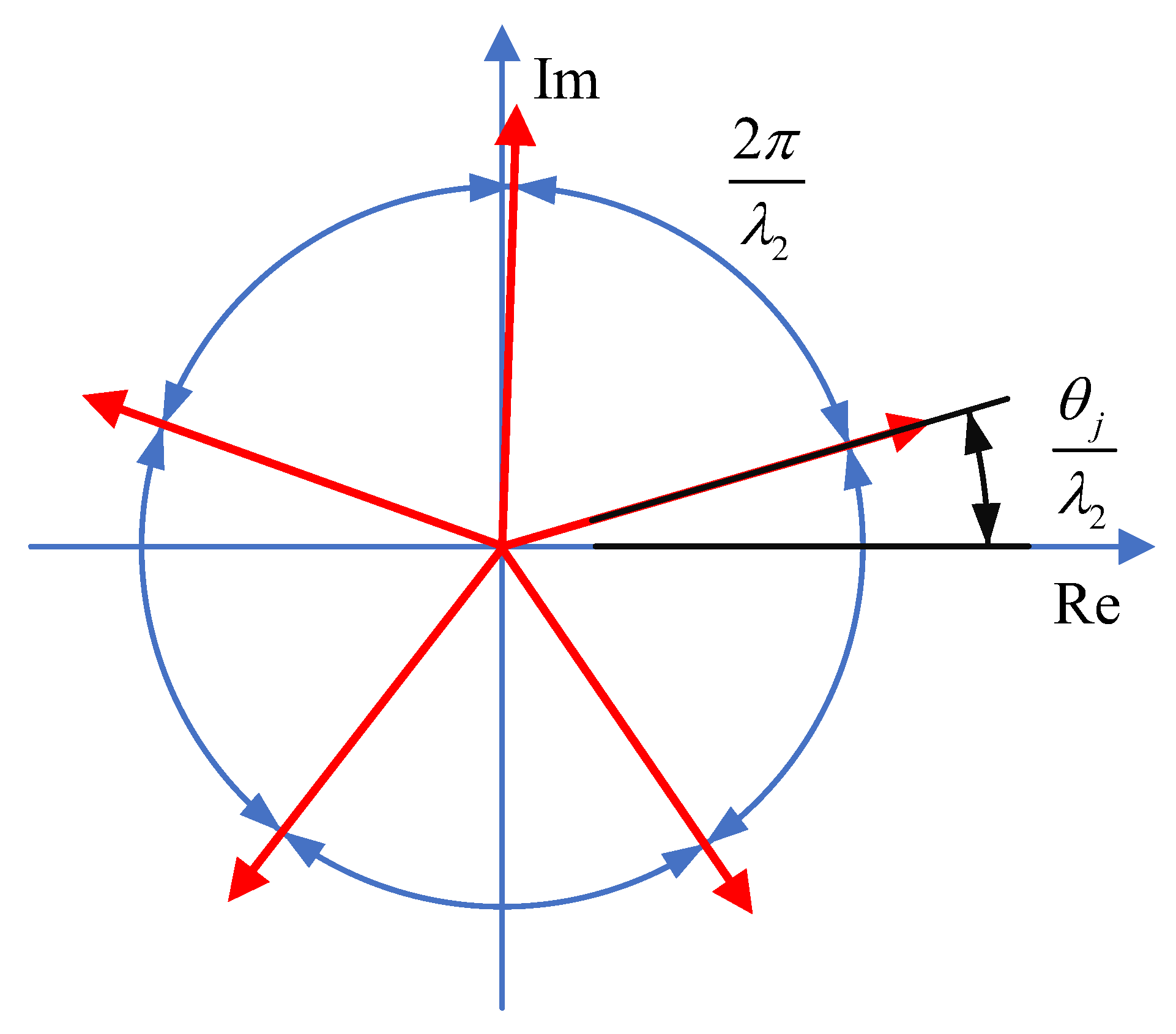
3.1. Stability Analysis of FOESO-ADRC

In this section, the stability criteria of the FOESO and FOESO-based ADRC system are provided. As shown in Figure 2, the stability of the FOESO with the PD controller is equal to the state observer-based feedback controller. Assume the controller output

$$u=r-\left(\begin{array}{cc}{k}_1& k_2\end{array}\right){\left(\begin{array}{cc}{z}_1& z_2\end{array}\right)}^T-k_3{z}_3$$

(18)

$u_0=r-\left(\begin{array}{cc}{k}_1& k_2\end{array}\right){\left(\begin{array}{cc}{z}_1& z_2\end{array}\right)}^T$ is the general form of state observer-based feedback controller output expression. $u_1=-k_3{z}_3$ is the compensation signal which is aiming to cancel the influence of total disturbance. According to Equation (16), we choose $k_3=1/b_0$, so the state-space equation can be written as:

$$\dot{x}=\left(\begin{array}{cc}0& 1\\ -a_{1,\alpha }& -a_{0,\alpha }\end{array}\right)x+\left(\begin{array}{c}0\\ b\end{array}\right)\left(r-\left(\begin{array}{cc}{k}_1& k_2\end{array}\right){\left(\begin{array}{cc}{z}_1& z_2\end{array}\right)}^T\right)+\left(\begin{array}{c}0\\ b\end{array}\right)\left(\frac{f_{\alpha }}{b}-\frac{z_3}{b}\right)$$

If the estimation of the FOESO is timely and accurate, the total disturbance will be compensated immediately.

From (16) and (17), the augmented state-space equation of the control system can be written as

$$\left(\begin{array}{c}\dot{x}\\ \dot{z}\end{array}\right)=\left(\begin{array}{cc}A& 0\\ HC& \tilde{A}-H\tilde{C}\end{array}\right)\left(\begin{array}{c}x\\ z\end{array}\right)+\left(\begin{array}{c}B\\ \tilde{B}\end{array}\right)u+\left(\begin{array}{c}B\\ 0\end{array}\right)\frac{f_{\alpha }}{b}$$

(19)

Substitute Equation (18) into Equation (19), the state-space equation can be written as

$$\left(\begin{array}{c}\dot{x}\\ \dot{z}\end{array}\right)=\left(\begin{array}{cc}A& -BK\\ HC& \tilde{A}-\tilde{B}K-H\tilde{C}\end{array}\right)\left(\begin{array}{c}x\\ z\end{array}\right)+\left(\begin{array}{c}B\\ \tilde{B}\end{array}\right)r+\left(\begin{array}{c}B\\ 0\end{array}\right)\frac{f_{\alpha }}{b}$$

(20)

where $A=\left(\begin{array}{cc}0& 1\\ -a_{1,\alpha }& -a_{0,\alpha }\end{array}\right)$, $\tilde{A}=\left(\begin{array}{cc}A& 0_{2\times 1}\\ 0_{1\times 2}& 0\end{array}\right)$, $z={\left(\begin{array}{ccc}{z}_1& z_2& z_3\end{array}\right)}^T$, $B={\left(\begin{array}{cc}0& 1/I_{zz}\end{array}\right)}^T$, $\tilde{B}={\left(\begin{array}{cc}0& 1/I_{zz}\end{array}\right)}^T$, $K=\left(\begin{array}{ccc}{k}_1& k_2& 1/b\end{array}\right)$, $H={\left(\begin{array}{ccc}{\beta }_1{\left(\frac{D}{Dt}\right)}^{{\alpha }_e}& {\beta }_2{\left(\frac{D}{Dt}\right)}^{{\beta }_e}& {\beta }_3{\left(\frac{D}{Dt}\right)}^{{\gamma }_e}\end{array}\right)}^T$, $C=\left(\begin{array}{cc}1& 0\end{array}\right)$, $\tilde{C}=\left(\begin{array}{ccc}1& 0& 0\end{array}\right)$.

Define state transformation as follows:

$$\left(\begin{array}{c}x\\ z_{st}\end{array}\right)=P\left(\begin{array}{c}x\\ z\end{array}\right)$$

(21)

where $P=\left(\begin{array}{cc}{I}_{2\times 2}& 0\\ J& -I_{3\times 3}\end{array}\right)$, $J=\left(\begin{array}{cc}1& 0\\ 0& 1\\ 0& 0\end{array}\right)$

According to (16) and (17), the transferred state-space equation can be written as

$$\left(\begin{array}{c}\dot{x}\\ {\dot{z}}_{st}\end{array}\right)=\left(\begin{array}{cc}A& 0\\ 0& \tilde{A}\end{array}\right)\left(\begin{array}{c}x\\ z_{st}\end{array}\right)+\left(\begin{array}{cc}-BKJ& BK\\ 0& 0\end{array}\right)\left(\begin{array}{c}x\\ z_{st}\end{array}\right)+\left(\begin{array}{cc}0& 0\\ 0& H\tilde{C}\end{array}\right)\left(\begin{array}{c}x\\ z_{st}\end{array}\right)+\left(\begin{array}{c}B\\ 0\end{array}\right)r+\left(\begin{array}{c}B\\ \tilde{B}\end{array}\right)\frac{f_{\alpha }}{b}$$

(22)

Using inverse Laplace transform, the transfer function matrix can be written as:

$$\left(\begin{array}{c}X\\ Z_{st}\end{array}\right)=\frac{1}{M_1\left(s\right)·M_2\left(s\right)}\left(\begin{array}{cc}{T}_{11}& T_{12}\\ 0& T_{22}\end{array}\right)\left(\left(\begin{array}{c}B\\ 0\end{array}\right)R+\left(\begin{array}{c}B\\ \tilde{B}\end{array}\right)\left(\frac{F_d}{b}\right)\right)$$

(23)

where $M_1\left(s\right)=s^2+b{k}_{2}s+b{k}_1$, $M_2\left(s\right)=s^3+{\beta }_1{s}^{2+{\alpha }_e}+{\beta }_2{s}^{1+{\beta }_e}+{\beta }_3{s}^{{\gamma }_e}$, $T_{11}=\left(\begin{array}{cc}s+b{k}_1& 1\\ -b{k}_1& s\end{array}\right)$, $T_{22}=\left(\begin{array}{ccc}{s}^2& s& 1\\ -{\beta }_2{s}^{1+{\beta }_f}-{\beta }_3{s}^{{\gamma }_f}& s^2+{\beta }_1{s}^{1+{\alpha }_f}& s+{\beta }_1{s}^{{\alpha }_f}\\ -{\beta }_3{s}^{1+{\gamma }_f}& -{\beta }_3{s}^{{\gamma }_f}& s^2+{\beta }_1{s}^{1+{\alpha }_f}+{\beta }_2{s}^{{\beta }_f}\end{array}\right)$, $T_{12}=T_{11}BK{T}_{22}$.

The characteristic equation of the control system is $M\left(s\right)=M_1\left(s\right)·M_2\left(s\right)$.

Lemma 1

([29]). For a fractional-order system such as $G_{fo}\left(s\right)=\frac{{\displaystyle \sum d_i\left(s^{1/{\lambda }_1}\right)}}{{\displaystyle \prod \left(s^{1/{\lambda }_1}-{\tau }_j\right)}}$, if choosing parameters $d_i$ and ${\tau }_i$ to assure $\left|\arg \left({\omega }_j\right)\right|>\frac{\pi }{2{\lambda }_1}$, where ${\omega }_j$ is an arbitrary root of ${\displaystyle \prod \left(\omega -{\tau }_j\right)}=0$, then the fractional-order system is stable.

If we want to prove system (21) is stable based on Lemma 1, the transfer function should be written as $G_{fo}\left(s\right)=\frac{{\displaystyle \sum d_i\left(s^{1/{\lambda }_1}\right)}}{{\displaystyle \prod \left(s^{1/{\lambda }_1}-{\tau }_j\right)}}$, and the equation ${\displaystyle \prod \left(\omega -{\tau }_j\right)}=0$ should be solved. Compared with the characteristic equation M₁ (s) = 0 and M₂ (s) = 0, there are too many extra roots. To simplify the proof process, we can prove that a different fractional-order system series is stable when each component’s systems are stable.

Theorem 1.

For a fractional-order system such as$G_{fo}\left(s\right)=\frac{{\displaystyle \sum d_i\left(s^{1/{\lambda }_1}\right)}}{{\displaystyle \prod \left(s^{1/{\lambda }_1}-{\tau }_j\right)}}·\frac{{\displaystyle \sum d_k\left(s^{1/{\lambda }_2}\right)}}{{\displaystyle \prod \left(s^{1/{\lambda }_2}-{\tau }_l\right)}}$, if choosing parameters$d_i$, d_k, τ_jandτ_lto assure$\left|\arg \left({\omega }_j\right)\right|>\frac{\pi }{2{\lambda }_2}$and $\left|\arg \left({\omega }_l\right)\right|>\frac{\pi }{2{\lambda }_2}$, where ω_j is an arbitrary root of${\displaystyle \prod \left(\omega -{\tau }_j\right)}=0$and ω_l is an arbitrary root of${\displaystyle \prod \left(\omega -{\tau }_l\right)}=0$, then the fractional-order system is stable.

Proof. 

The characteristic equation of the fractional-order system can be written as:

$$M_p\left(s\right)={\displaystyle \prod \left({\left(s^{1/{\lambda }_1{\lambda }_2}\right)}^{{\lambda }_2}-{\tau }_j\right)}·{\displaystyle \prod \left({\left(s^{1/{\lambda }_1{\lambda }_2}\right)}^{{\lambda }_1}-{\tau }_l\right)}$$

Define ${\overline{M}}_p\left(\omega \right)={\displaystyle \prod \left({\omega }^{{\lambda }_2}-{\tau }_j\right)}·{\displaystyle \prod \left({\omega }^{{\lambda }_1}-{\tau }_l\right)}$. ${\omega }_{j{k}_1}=A_{j{k}_1}{e}^{i{\theta }_{j{k}_1}}$ is the root of $\left({\omega }^{{\lambda }_2}-{\tau }_j\right)=0$, $k_1=1,\cdots ,{\lambda }_1$. ${\omega }_{l{k}_2}=A_{l{k}_2}{e}^{i{\theta }_{l{k}_2}}$ is the root of $\left({\omega }^{{\lambda }_2}-{\tau }_j\right)=0$, $k_2=1,\cdots ,{\lambda }_2$.

${\omega }_j$ can be written as ${\omega }_j=A_j{e}^{i{\theta }_j}$, ${\theta }_j\in \left[\begin{array}{cc}-\pi & \pi \end{array}\right)$.

It is easy to proof:

$${\left({\omega }_{j{k}_1}\right)}^{{\lambda }_2}={\omega }_j$$

(24)

Combine line259, line261 and the definition of ${\omega }_{j{k}_1}$, we can obtain $A_j{e}^{i{\theta }_j}={\left(A_{j{k}_1}\right)}^{{\lambda }_2}{e}^{i{\lambda }_2{\theta }_{j{k}_1}}$, ${\theta }_j,{\theta }_{j{k}_1}\in \left[\begin{array}{cc}-\pi & \pi \end{array}\right]$

$$A_{j{k}_1}=\sqrt[{\lambda }_2]{A_j}$$

$${\theta }_{j{k}_1}=\frac{{\theta }_j\pm 2k\pi }{{\lambda }_2}, k=0,\cdots ,\mathrm{floor}\left({\lambda }_2/2\right)$$

where floor (x) indicates round-down function:

$$y=\mathrm{floor}\left(x\right), y\in \mathbb{Z}, y\le x<y+1$$

The ${\omega }_{j{k}_1}$ can be illustrated in complex plane as Figure 3.

Assume ${\theta }_j>0$. We can divide ${\omega }_{j{k}_1}$ into two categories to discuss separately.

For ${\theta }_{j{k}_1}=\frac{{\theta }_j}{{\lambda }_2}+\frac{2k}{{\lambda }_2}\pi$, according to line265, if λ₂ is an odd number, then $k=0,\cdots ,\left({\lambda }_2-1\right)/2$, ${\theta }_{j{k}_1}\in \left[\begin{array}{cc}\frac{{\theta }_j}{{\lambda }_2},& \frac{{\theta }_j}{{\lambda }_2}+\frac{\left({\lambda }_2-1\right)}{{\lambda }_2}\pi \end{array}\right]$. Known ${\theta }_j\in \left[\begin{array}{cc}0& \pi \end{array}\right]$, ${\theta }_j>\frac{\pi }{2{\lambda }_1}$, we can obtain $\frac{{\theta }_j}{{\lambda }_2}+\frac{\left({\lambda }_2-1\right)}{{\lambda }_2}\pi \le \pi$. Then, $\left|\arg \left({\omega }_{j{k}_1}\right)\right|\in \left[\begin{array}{cc}\frac{\pi }{2{\lambda }_1{\lambda }_2},& \frac{\pi }{2{\lambda }_1{\lambda }_2}+\frac{\left({\lambda }_2-1\right)}{{\lambda }_2}\pi \end{array}\right]$. $\min \left(\left|\arg \left({\omega }_{j{k}_1}\right)\right|\right)>\frac{\pi }{2{\lambda }_1{\lambda }_2}$ ${\omega }_{j{k}_1}$ satisfies the stable condition of Lemma 1.

If λ₂ is an even number, then $k=0,\cdots ,{\lambda }_2/2$. For $k=0,\cdots ,\left({\lambda }_2-2\right)/2$, corresponding ${\theta }_{j{k}_1}\in \left[\begin{array}{cc}\frac{{\theta }_j}{{\lambda }_2},& \frac{{\theta }_j}{{\lambda }_2}+\frac{\left({\lambda }_2-2\right)}{{\lambda }_2}\pi \end{array}\right]$, $\min \left(\left|\arg \left({\omega }_{j{k}_1}\right)\right|\right)=\frac{{\theta }_j}{{\lambda }_2}$. For $k={\lambda }_2/2$, corresponding $\pi <{\theta }_{j{k}_1}=\frac{{\theta }_j}{{\lambda }_2}+\pi <2\pi$, then the $\left|\arg \left({\omega }_{j{k}_1}\right)\right|$ can be expressed as $\left|\arg \left({\omega }_{j{k}_1}\right)\right|=2\pi -{\theta }_{j{k}_1}=\pi -\frac{{\theta }_j}{{\lambda }_2}$. Known ${\theta }_j\in \left[\begin{array}{cc}0& \pi \end{array}\right]$, ${\lambda }_2\ge 2$, we can obtain $\min \left(\left|\arg \left({\omega }_{j{k}_1}\right)\right|\right)=\pi -\frac{{\theta }_j}{{\lambda }_2}\ge \frac{{\theta }_j}{{\lambda }_2}>\frac{\pi }{2{\lambda }_1{\lambda }_2}$. ${\omega }_{j{k}_1}$ satisfies the stable condition of Lemma 1.

For ${\theta }_{j{k}_1}=\frac{{\theta }_j}{{\lambda }_2}-\frac{2k}{{\lambda }_2}\pi$, if λ₂ is an odd number, we can obtain ${\theta }_{j{k}_1}\in \left[\begin{array}{cc}\frac{{\theta }_j}{{\lambda }_2}-\frac{\left({\lambda }_2-1\right)}{{\lambda }_2}\pi ,& \frac{{\theta }_j}{{\lambda }_2}\end{array}\right]$. For k = 0, the corresponding ${\theta }_{j{k}_1}=\frac{{\theta }_j}{{\lambda }_2}>0$. For $k=1,\cdots ,\left({\lambda }_2-1\right)/2$, the corresponding ${\theta }_{j{k}_1}\in \left[\begin{array}{cc}\frac{{\theta }_j}{{\lambda }_2}-\frac{\left({\lambda }_2-1\right)}{{\lambda }_2}\pi ,& \frac{{\theta }_j}{{\lambda }_2}-\frac{2}{{\lambda }_2}\pi \end{array}\right]$. $-\pi <\frac{{\theta }_j}{{\lambda }_2}-\frac{\left({\lambda }_2-1\right)}{{\lambda }_2}\pi <\frac{{\theta }_j}{{\lambda }_2}-\frac{2}{{\lambda }_2}\pi <0$

So, the $\min \left(\left|\arg \left({\omega }_{j{k}_1}\right)\right|\right)=\min \left(\begin{array}{cc}\left|\frac{{\theta }_j}{{\lambda }_2}\right|,& \left|\frac{{\theta }_j}{{\lambda }_2}-\frac{2}{{\lambda }_2}\pi \right|\end{array}\right)$. Known $0<{\theta }_j\le \pi$, we can obtain $\left|\frac{{\theta }_j}{{\lambda }_2}-\frac{2}{{\lambda }_2}\pi \right|\ge \left|\frac{1}{{\lambda }_2}\pi -\frac{2}{{\lambda }_2}\pi \right|=\frac{1}{{\lambda }_2}\pi \ge {\theta }_j$. The $\min \left(\left|\arg \left({\omega }_{j{k}_1}\right)\right|\right)$ can be written as $\min \left(\left|\arg \left({\omega }_{j{k}_1}\right)\right|\right)=\frac{{\theta }_j}{{\lambda }_2}>\frac{\pi }{2{\lambda }_1{\lambda }_2}$. ${\omega }_{j{k}_1}$ satisfies the stable condition of Lemma 1.

If λ₂ is an even number, we can obtain ${\theta }_{j{k}_1}\in \left[\begin{array}{cc}\frac{{\theta }_j}{{\lambda }_2}-\pi ,& \frac{{\theta }_j}{{\lambda }_2}\end{array}\right]$. For $k=0$, the corresponding ${\theta }_{j{k}_1}=\frac{{\theta }_j}{{\lambda }_2}>0$. For $k=1,\cdots ,{\lambda }_2/2$, the corresponding ${\theta }_{j{k}_1}\in \left[\begin{array}{cc}\frac{{\theta }_j}{{\lambda }_2}-\pi ,& \frac{{\theta }_j}{{\lambda }_2}-\frac{2}{{\lambda }_2}\pi \end{array}\right]$, where $-\pi <\frac{{\theta }_j}{{\lambda }_2}-\pi <\frac{{\theta }_j}{{\lambda }_2}-\frac{2}{{\lambda }_2}\pi \le -\frac{{\theta }_j}{{\lambda }_2}$. Therefore, we can obtain $\min \left(\left|\arg \left({\omega }_{j{k}_1}\right)\right|\right)=\frac{{\theta }_j}{{\lambda }_2}>\frac{\pi }{2{\lambda }_1{\lambda }_2}$. ${\omega }_{j{k}_1}$ satisfies the stable condition of Lemma 1.

Conclusion 1.

From the comprehensive conclusions above, we can obtain that for θ_j > 0, if the characteristic equation${\displaystyle \prod \left({\omega }_j-{\tau }_j\right)}=0$satisfies the stable condition in Lemma 1, the corresponding roots of${\displaystyle \prod \left({\left({\omega }_{j{k}_1}\right)}^{{\lambda }_2}-{\tau }_j\right)}=0$satisfied the stable condition of${\omega }_{j{k}_1}>\frac{\pi }{2{\lambda }_1{\lambda }_2}$in Lemma 1. The similar conclusion while θ_j < 0 can be proof in a similar way.

Based on the above conclusion, for the system $G_{fo}\left(s\right)=\frac{{\displaystyle \sum d_i\left(s^{1/{\lambda }_1}\right)}}{{\displaystyle \prod \left(s^{1/{\lambda }_1}-{\tau }_j\right)}}·\frac{{\displaystyle \sum d_k\left(s^{1/{\lambda }_2}\right)}}{{\displaystyle \prod \left(s^{1/{\lambda }_2}-{\tau }_l\right)}}$, the denominator of the transfer function can be written as $M_p\left(s\right)={\displaystyle \prod \left({\left(s^{1/{\lambda }_1{\lambda }_2}\right)}^{{\lambda }_2}-{\tau }_j\right)}·{\displaystyle \prod \left({\left(s^{1/{\lambda }_1{\lambda }_2}\right)}^{{\lambda }_1}-{\tau }_l\right)}$.

If $\left|\arg \left({\omega }_j\right)\right|>\frac{\pi }{2{\lambda }_1}$ and $\left|\arg \left({\omega }_l\right)\right|>\frac{\pi }{2{\lambda }_2}$, where ω_j is an arbitrary root of ${\displaystyle \prod \left(\omega -{\tau }_j\right)}=0$ and ω_l is an arbitrary root of ${\displaystyle \prod \left(\omega -{\tau }_l\right)}=0$, we can obtain $\left|\arg \left({\omega }_{jk3}\right)\right|>\frac{\pi }{2{\lambda }_1{\lambda }_2}$, where ${\omega }_{jk3}$ are the roots of ${\displaystyle \prod \left({\omega }^{{\lambda }_2}-{\tau }_j\right)}·{\displaystyle \prod \left({\omega }^{{\lambda }_1}-{\tau }_l\right)}=0$. The system satisfies the stable condition. □

3.2. Parameter Tuning

For the system

$$\left(\begin{array}{c}\mathit{X}\\ {\mathit{Z}}_{st}\end{array}\right)=\frac{1}{M_1\left(s\right)·M_2\left(s\right)}\left(\begin{array}{cc}{\mathit{T}}_{11}& {\mathit{T}}_{12}\\ 0& {\mathit{T}}_{22}\end{array}\right)\left(\left(\begin{array}{c}\mathit{B}\\ 0\end{array}\right)R+\left(\begin{array}{c}\mathit{B}\\ \tilde{\mathit{B}}\end{array}\right)\left(\frac{F_d}{b}\right)\right)$$

Choosing $k_1=\frac{{\omega }_c^2}{b}$, $k_2=\frac{2{\omega }_c}{b}$, ${\beta }_1=3{\omega }_{ESO}$, ${\beta }_2=3{\omega }_{ESO}^2$, ${\beta }_3={\omega }_{ESO}^3$, ${\alpha }_e=1-\mu$, ${\beta }_e=2-2\mu$, ${\gamma }_e=3-3\mu$, where ${\omega }_c,{\omega }_{ESO}\in {\Re }^{+}$. Then, the transfer function can be written as:

$$\left(\begin{array}{c}\mathit{X}\\ {\mathit{Z}}_{st}\end{array}\right)=\frac{1}{{\left(s+{\omega }_c\right)}^2·{\left(s^{\mu }+{\omega }_{ESO}\right)}^3}\left(\begin{array}{cc}{\mathit{T}}_{11}& {\mathit{T}}_{12}\\ 0& {\mathit{T}}_{22}\end{array}\right)\left(\left(\begin{array}{c}\mathit{B}\\ 0\end{array}\right)R+\left(\begin{array}{c}\mathit{B}\\ \tilde{\mathit{B}}\end{array}\right)\left(\frac{F_d}{b}\right)\right)$$

and the roots of characteristic equation are on the negative real axis, the system is stable. The transfer function from total disturbance to the estimation of total disturbance can be written as $G_{f{z}_3}=\frac{{\left({\omega }_{ESO}\right)}^3}{{\left(s+{\omega }_c\right)}^2·{\left(s^{\mu }+{\omega }_{ESO}\right)}^3}$. Tuning the parameter μ can alter the decline rate of the amplitude–frequency curve. The bode diagram of $G_{f{z}_3}$ with the same ω_c, ω_ESO and different μ is shown in the figure, where $\mu =1$ indicates the integral-order ESO.

As shown in Figure 4, for the total disturbance estimation, when the frequency is lower than the bandwidth, the fractional-order parameter μ has a insignificant influence on the frequency-domain characteristics. When the frequency is higher than the bandwidth, the decline rate of the magnitude–frequency curve raises approximately proportional to the increase in the fractional-order parameter μ. The frequency-domain characteristics of the noise response are similar to the total disturbance. The attenuation of the high-frequency measurement noise will be significant if a larger μ is chosen.

It illustrates that we could alter the magnitude–frequency characteristic of the ESO by tuning the fractional-order parameter μ. And the result seems it could not be realized by tuning the bandwidth.

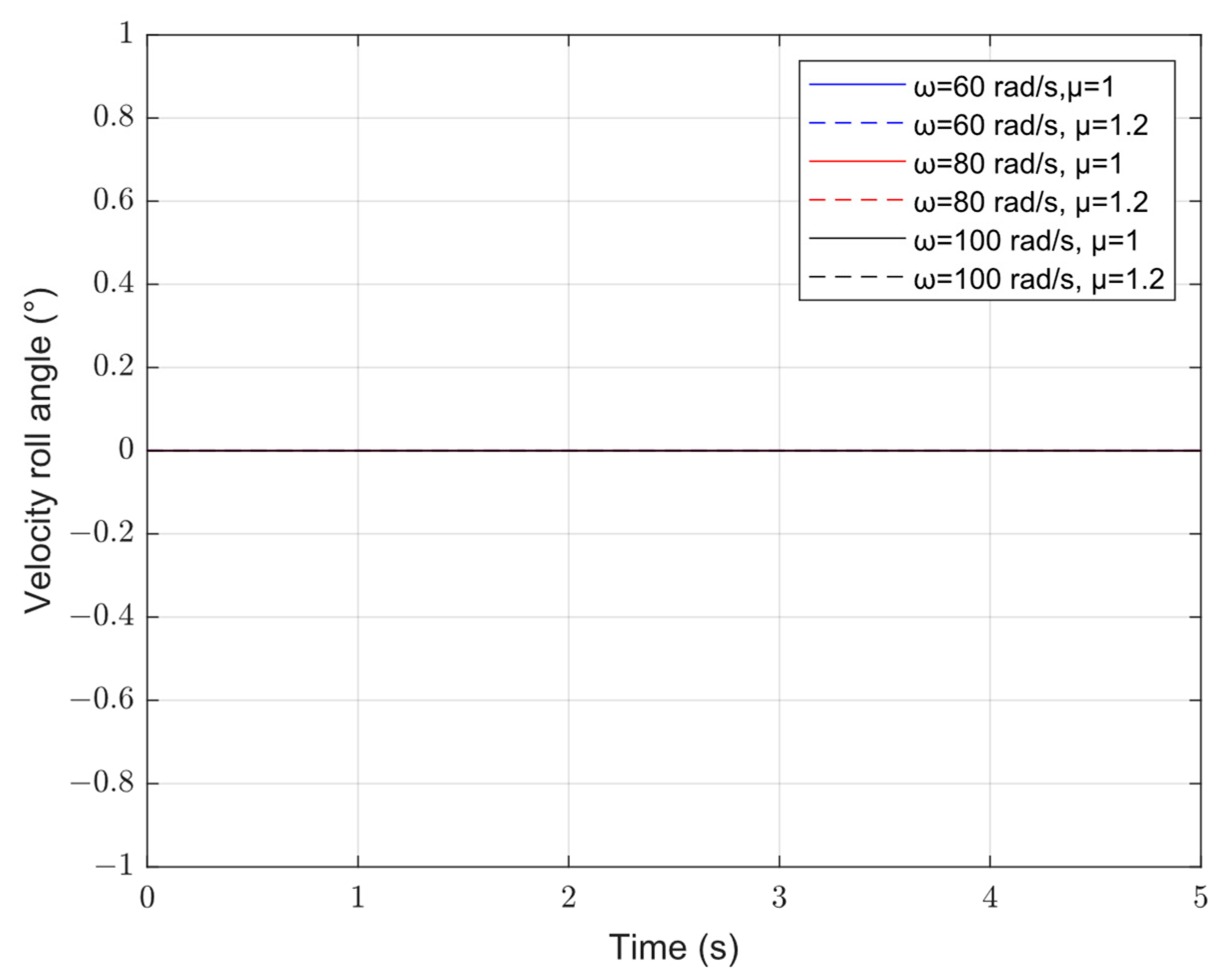
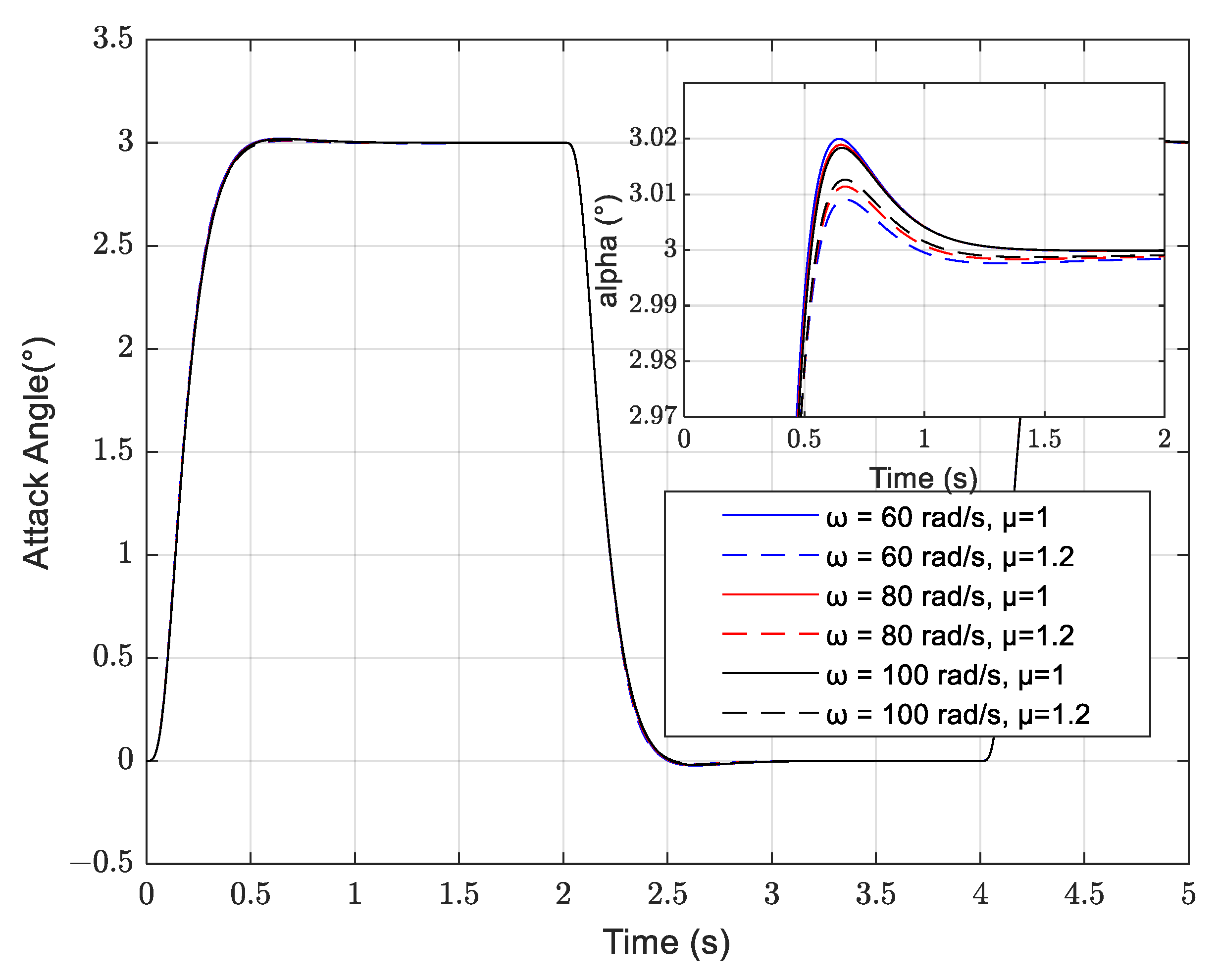
4. Simulation Analysis

In this section, we will show the control performance of the FOESO-based ADRC. According to the linearized model in Section 2, the flight states are necessary for the controller design. The initial flight states are set in

Table 2. Initial Flight Status.

Parameters	Value	Parameters	Value
Altitude	33.5 km	Attack angle	0°
Velocity	15 Ma	Sideslip angle	0°
Path angle	0°	Velocity roll angle	0°
Path azimuth angle	0°

.

According to the linearized model, the parameters of the PID controller are tuned as in

Table 3. Parameters of PID Controller.

Parameters	Roll	Yaw	Pitch
Kp	119.5	74.9	198.7
Ki	10.1	0	1.65
Kd	20.1	17.4	19.4

.

For the fair comparison of the FOESO and ESO, the initial flight status and the control parameters shown in Table 2 and Table 3 are used in all the following simulations. Only the parameters of the FOESO and ESO are altered to illustrate the effectiveness of the FOESO.

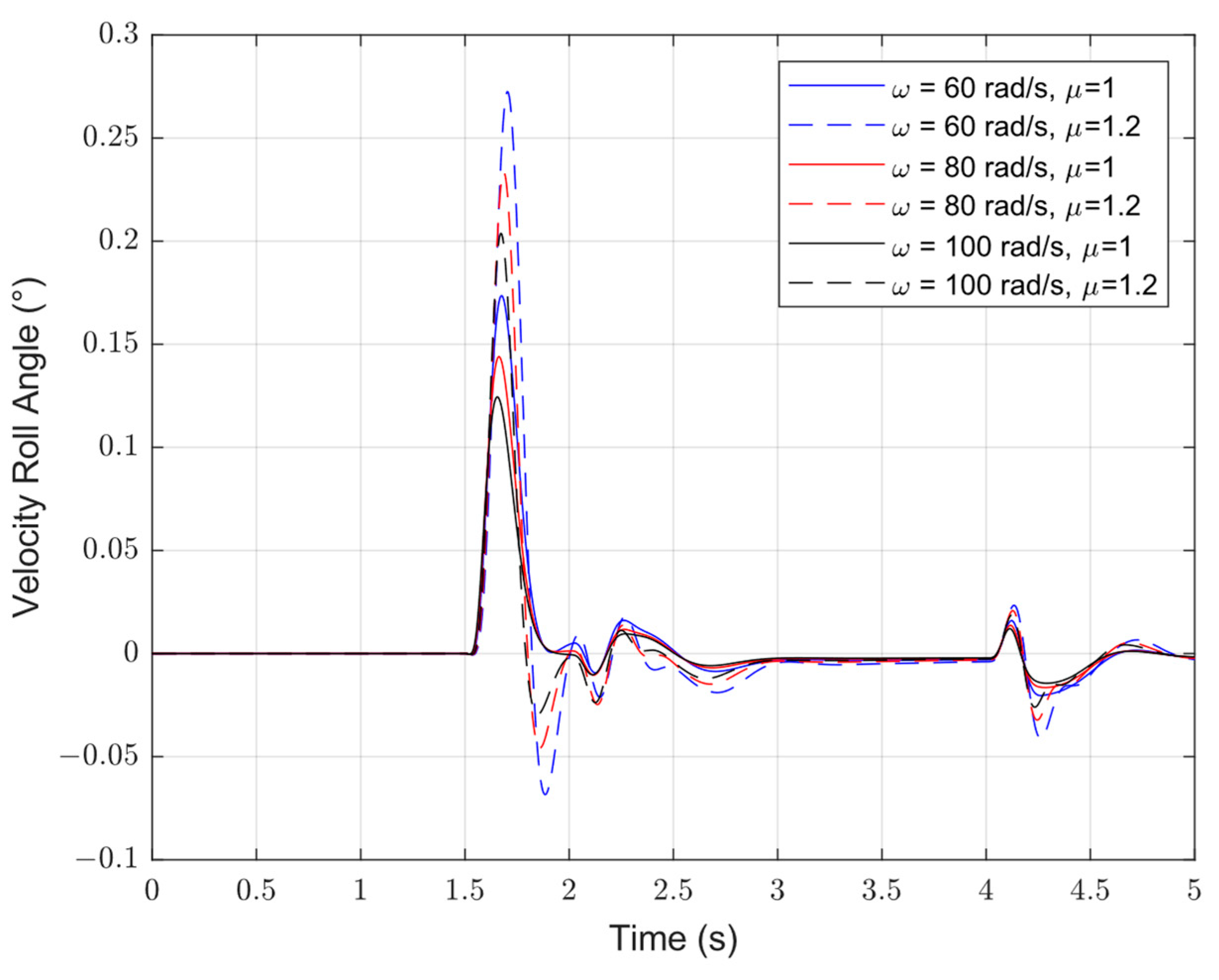
4.1. FOESO Versus ESO: Nominal Situation

As shown in Figure 4, any μ > 1 induces the magnitude decreasing faster at the middle-frequency band. It brings a better noise suppression and potentially performance degradation. To assess the influence of μ, the comparation of the FOESO and ESO-based ADRC is proposed. The nonlinear model is considered accurate. It means that the external disturbance does not exist. In addition, the total disturbance is equal to the modeling errors between the linearized model and the nonlinear model. The HV attitude control system is simulated. The expected velocity roll angle, sideslip angle and attack angle are set to 0, 0, and the rectangular wave has an amplitude of 3. The simulation results are shown in Figure 5, Figure 6, Figure 7 and Figure 8.

Figure 5 and Figure 6 show that the controller of the roll channel and yaw channel are stable. We can assess the influence of μ according to Figure 7, in which the response of the attack angle with μ = 1 is similar to the response with μ = 1.2. The introduction of fractional-order calculus could enhance the anti-noise ability and show a non-significant influence on the control performance in the nominal system.

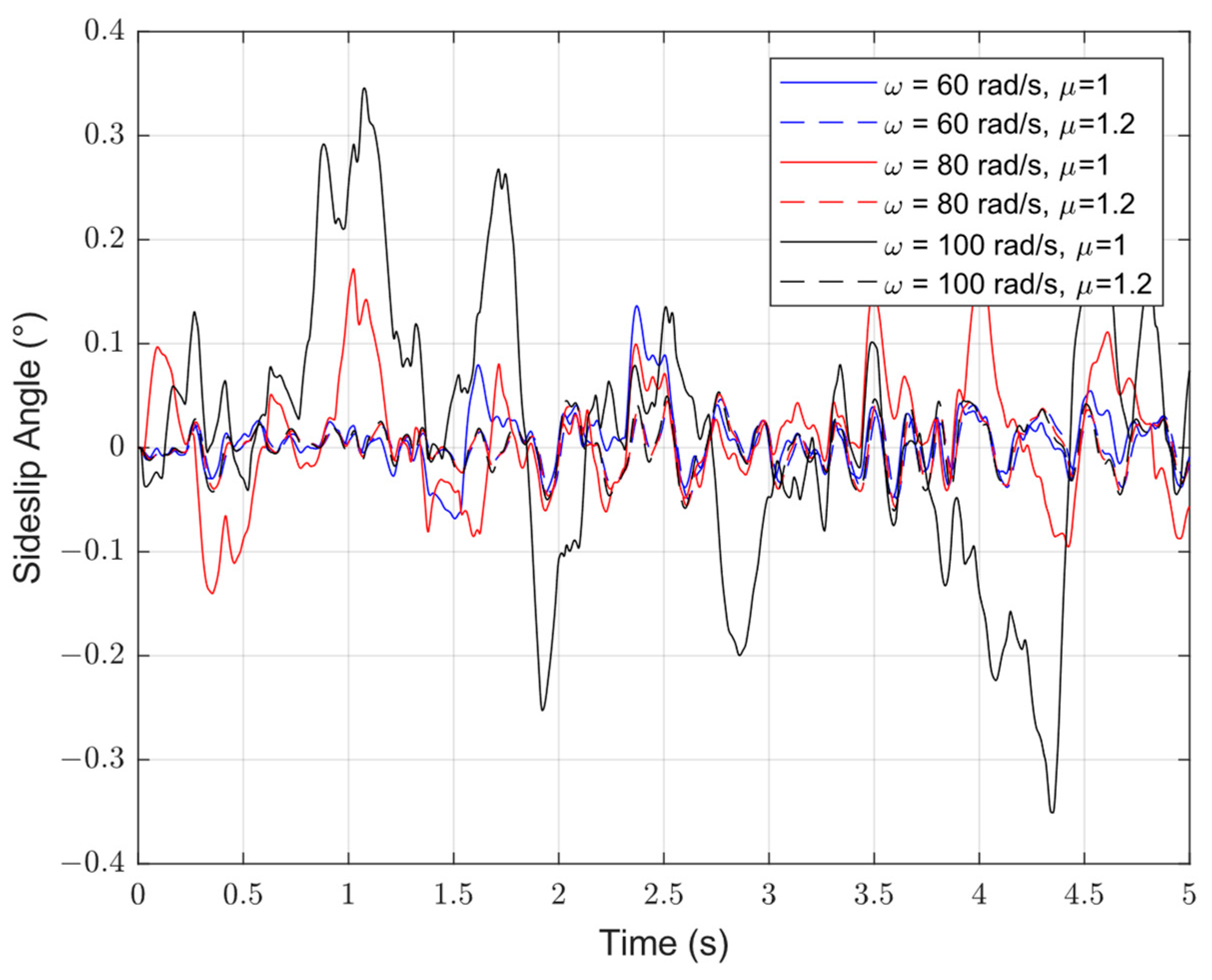
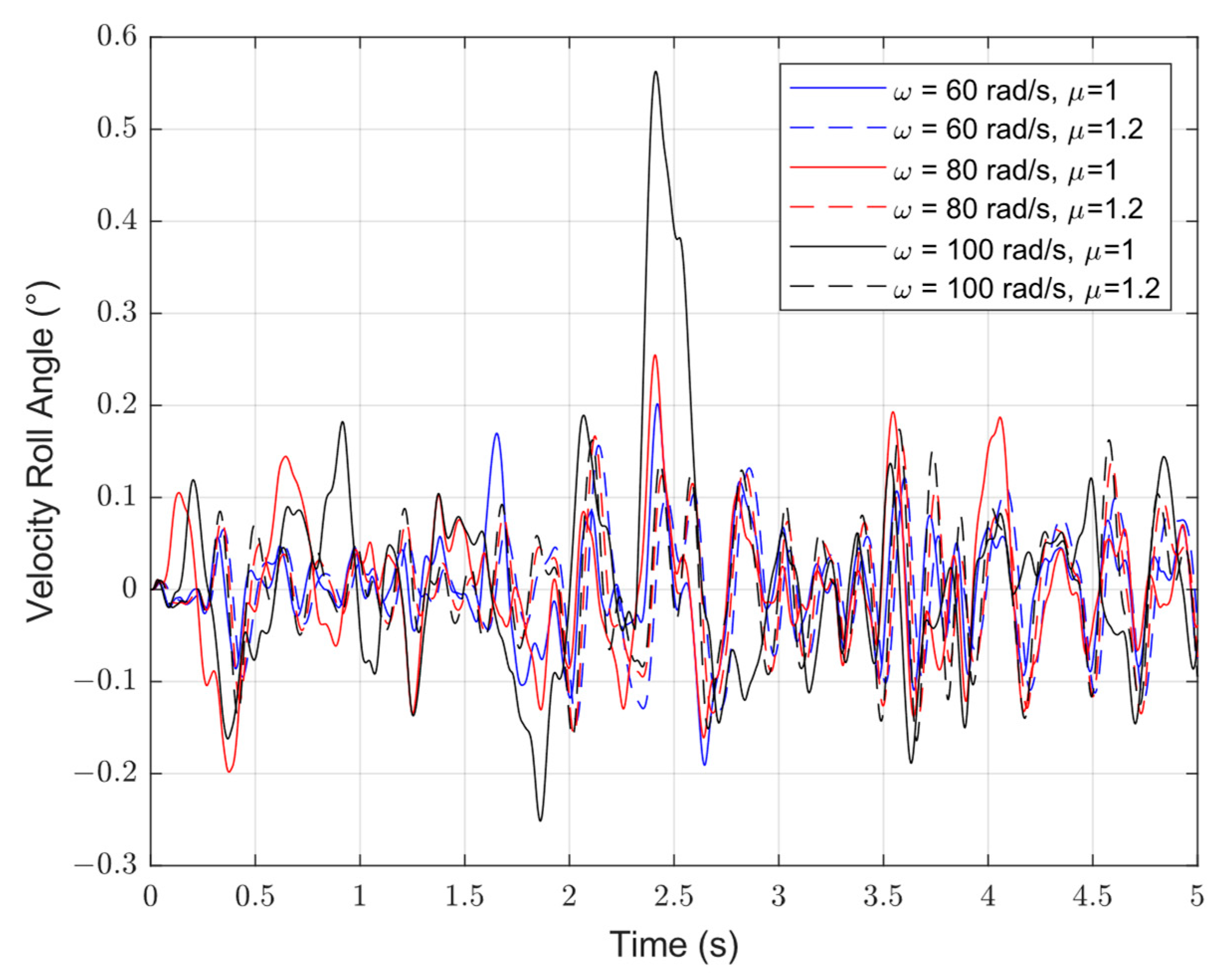
4.2. FOESO Versus ESO: Measurement Noise Situation

Within a rational range, to increase the bandwidth of the ESO will significantly improve the performance of the ESO and ADRC. Nonetheless, this result assumes that the control system is noise-free. This is impractical. In the presence of a stochastic measurement noise, the impact will become more significant as the result of the increasing ESO bandwidth. The measurement noise is applied to three channels. In addition, the variance is set to 0.002. The simulation of the HV with measurement noise is studied. The results are shown as follows.

As shown in Figure 8, Figure 9 and Figure 10, the blue, red and black solid lines indicate the responses of the system with an ESO bandwidth of 60 rad/s, 80 rad/s and 100 rad/s. It can be seen that with the bandwidth increasing, the control performance is decreasing. The maximum errors of the three channels are shown in

Table 4. Maximum Error of Alpha.

	Integrated Order	Error	Fractional Order	Error
Attack Angle	ω = 60 rad/s	0.17°	ω = 60 rad/s	0.03°
	ω = 80 rad/s	0.3°	ω = 80 rad/s	0.05°
	ω = 100 rad/s	0.5°	ω = 100 rad/s	0.1°
Sideslip Angle	ω = 60 rad/s	0.13°	ω = 60 rad/s	0.06°
	ω = 80 rad/s	0.17°	ω = 80 rad/s	0.06°
	ω = 100 rad/s	0.34°	ω = 100 rad/s	0.06°
Velocity Roll Angle	ω = 60 rad/s	0.2°	ω = 60 rad/s	0.14°
	ω = 80 rad/s	0.25°	ω = 80 rad/s	0.13°
	ω = 100 rad/s	0.56°	ω = 100 rad/s	0.1°

.

The blue, red and black dotted lines indicate the attack angle response of the system with an FOESO bandwidth of 60 rad/s, 80 rad/s and 100 rad/s and a fractional-order parameter μ = 1.2. The maximum error of alpha is shown in Table 4. Apparently, compared with the ESO, the FOESO shows a significant ability to reduce the impact of the stochastic measurement noise.

Figure 11 shows the estimation of the total disturbance considering the measurement noise. The estimation performance of the system with larger bandwidth is less effective. In addition, the introduction of the fractional-order parameter μ can significantly suppress the measurement noise.

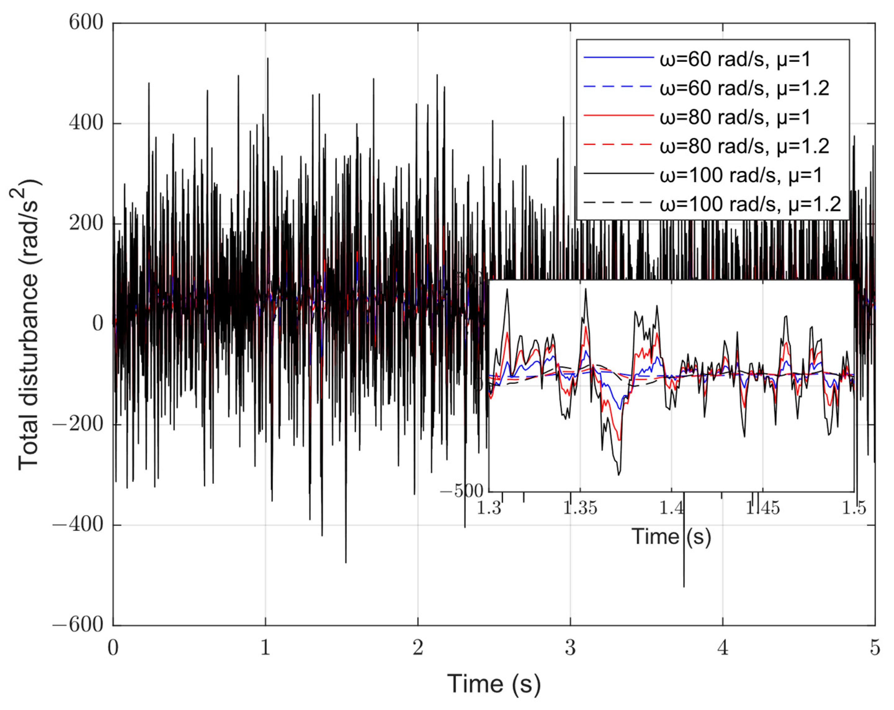
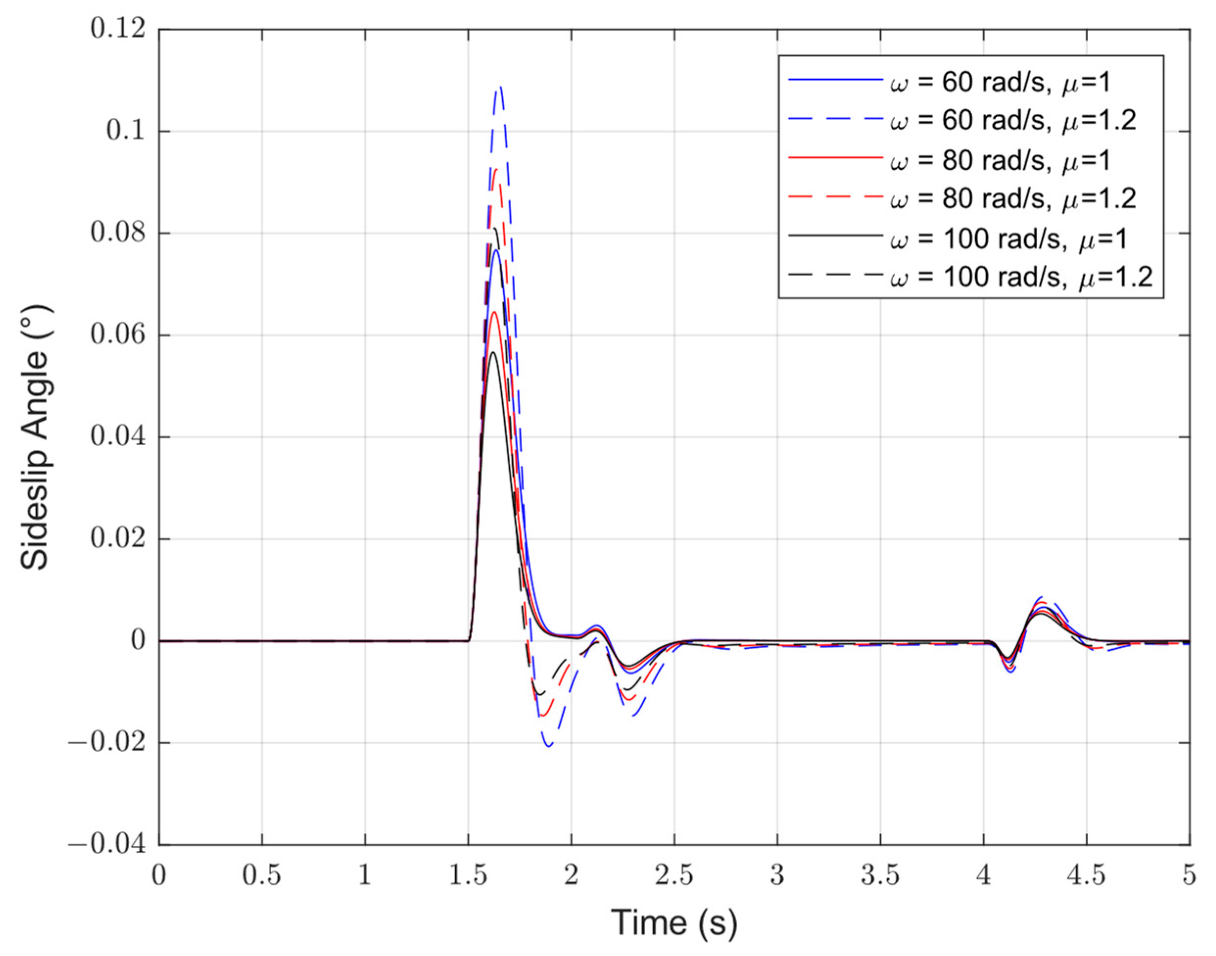
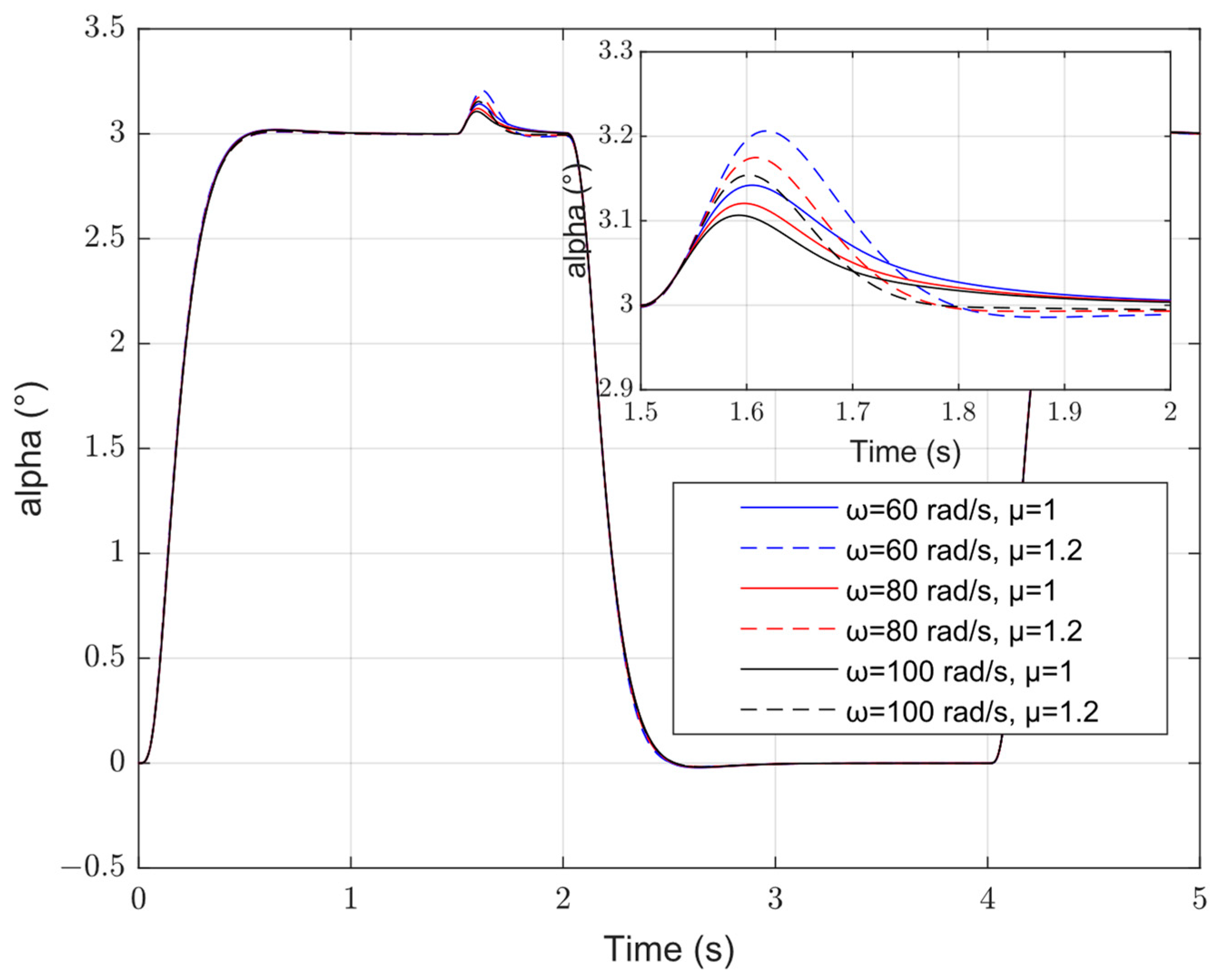
4.3. FOESO Versus ESO: Total Disturbance Situation

Except for the unmodeled dynamics, we introduce the external disturbance to assess the ability of the FOESO-based ADRC to estimate and compensate the total disturbance. The total disturbance can be expressed as follows:

$$\begin{array}{l}{f}_{\alpha }=f_{\alpha i}+f_{\alpha e}\\ f_{\beta }=f_{\beta i}+f_{\beta e}\end{array}$$

where $f_{\alpha e}=\{\begin{array}{cc}0,& t<1.5\\ 1500/I_{zz}& t\ge 1.5\end{array}$, $f_{\beta e}=\{\begin{array}{cc}0,& t<1.5\\ 500/I_{yy}& t\ge 1.5\end{array}$, represents simulation time. f_α, $f_{\alpha i}$ and f_αe indicate the total disturbance, internal disturbance and external disturbance of the pitch channel. f_β, f_βi and f_βe indicate the total disturbance, internal disturbance and external disturbance of the yaw channel. The simulation results are shown in Figure 12, Figure 13 and Figure 14.

Figure 12, Figure 13 and Figure 14 show that the FOESO-based ADRC has a larger overshoot and shorter setting time compared with the ESO with the same bandwidth. However, the bandwidth selection of the FOESO and ESO needs to consider the tradeoff of in the disturbance rejection performance and noise suppressing ability. The previous simulation shows that the FOESO with the bandwidth ω_ESO = 100 rad/s has a better noise suppressing ability compared with the ESO with the bandwidth ω_ESO = 60 rad/s. These two simulation results are shown in the figure as the blue solid line and black dotted line, respectively. We can see that the overshoot of the FOESO approach to the ESO and the setting time is much shorter.

Consequently, based on the previous simulation, the FOESO-based ADRC could have a better performance than the ESO considering the external disturbance and measurement noise. By introducing the fractional-order parameter μ, the FOESO could balance the control performance and the noise suppressing performance that the ESO could not realize.

5. Conclusions

In this paper, a novel fractional-order extended state observer is proposed. Compared with the traditional ESO, it can alter both the bandwidth and the decline rate of the amplitude–frequency curve without changing the total disturbance. The stable condition of the novel FOESO-based ADRC is given. The numerical simulation results have shown that the proposed novel FOESO has a significant advantage on the noise suppression. Considering both the total disturbance and measurement noise, the novel FOESO-based ADRC has the possibility to achieve a better tradeoff of the control performance and anti-noise ability.

References

1. Song, J.; Luo, Y.; Zhao, M.; Hu, Y.; Zhang, Y. Fault-Tolerant Integrated Guidance and Control Design for Hypersonic Vehicle Based on PPO. Mathematics 2022, 10, 3401. [Google Scholar] [CrossRef]
2. Qin, W.; Liu, J.; Liu, G.; He, B.; Wang, L. Robust parameter dependent receding horizon H∞ control of flexible air-breathing hypersonic vehicles with input constraints. Asian J. Control. 2015, 17, 508–522. [Google Scholar] [CrossRef]
3. Hu, X.; Wu, L.; Hu, C.; Wang, Z.; Gao, H. Dynamic output feedback control of a flexible air-breathing hypersonic vehicle via T–S fuzzy approach. Int. J. Syst. Sci. 2014, 45, 1740–1756. [Google Scholar] [CrossRef]
4. Bao, C.; Wang, P.; Tang, G. Integrated method of guidance, control and morphing for hypersonic morphing vehicle in glide phase. Chin. J. Aeronaut. 2021, 34, 535–553. [Google Scholar] [CrossRef]
5. Zhao, H.; Yang, L. Global adaptive neural backstepping control of a flexible hypersonic vehicle with disturbance estimation. Aircr. Eng. Aerosp. Technol. 2021, 94, 492–504. [Google Scholar] [CrossRef]
6. Song, J.; Wang, L.; Cai, G.; Qi, X. Nonlinear fractional order proportion-integral-derivative active disturbance rejection control method design for hypersonic vehicle attitude control. Acta Astronaut. 2015, 111, 160–169. [Google Scholar] [CrossRef]
7. Guo, F.; Lu, P. Improved adaptive integral-sliding-mode fault-tolerant control for hypersonic vehicle with actuator fault. IEEE Access 2021, 9, 143–151. [Google Scholar] [CrossRef]
8. Sun, H.; Li, S.; Sun, C. Finite time integral sliding mode control of hypersonic vehicles. Nonlinear Dyn. 2013, 73, 229–244. [Google Scholar] [CrossRef]
9. Han, J. From PID to Active Disturbance Rejection Control. IEEE Trans. Ind. Electron. 2009, 56, 900–906. [Google Scholar] [CrossRef]
10. Yoo, D.; Yau, S.; Gao, Z. Optimal fast tracking observer bandwidth of the linear extended state observer. Int. J. Control 2007, 80, 102–111. [Google Scholar] [CrossRef]
11. Razmjooei, H.; Palli, G.; Abdi, E. Continuous finite-time extended state observer design for electro-hydraulic systems. J. Frankl. Inst. 2022, 10, 5036–5055. [Google Scholar] [CrossRef]
12. Razmjooei, H.; Palli, G.; Nazari, M. Disturbance observer-based nonlinear feedback control for position tracking of electro-hydraulic systems in a finite time. Eur. J. Control. 2022, 67, 100659. [Google Scholar] [CrossRef]
13. Razmjooei, H.; Palli, G.; Abdi, E.; Strano, S.; Terzo, M. Finite-time continuous extended state observers: Design and experimental validation on electro-hydraulic systems. Mechatronics 2022, 85, 102812. [Google Scholar] [CrossRef]
14. Zhao, J.; Feng, D.; Cui, J.; Wang, X. Finite-Time Extended State Observer-Based Fixed-Time Attitude Control for Hypersonic Vehicles. Mathematics 2022, 10, 3162. [Google Scholar] [CrossRef]
15. Gao, K.; Song, J.; Wang, X.; Li, H. Fractional-order proportional-integral-derivative linear active disturbance rejection control design and parameter optimization for hypersonic vehicles with actuator faults. Tsinghua Sci. Technol. 2020, 26, 9–23. [Google Scholar] [CrossRef]
16. Sun, J.; Pu, Z.; Yi, J. Conditional disturbance negation based active disturbance rejection control for hypersonic vehicles. Control. Eng. Pract. 2019, 84, 159–171. [Google Scholar] [CrossRef]
17. Wei, W.; Zhang, Z.; Zuo, M. Phase leading active disturbance rejection control for a nanopositioning stage. ISA Trans. 2021, 116, 218–231. [Google Scholar] [CrossRef]
18. Doye, I.; Salama, K.; Laleg-Kirati, T. Robust fractional-order proportional-integral observer for synchronization of chaotic fractional-order systems. IEEE/CAA J. Autom. Sin. 2018, 6, 268–277. [Google Scholar] [CrossRef]
19. Doostdar, F.; Mojallali, H. An ADRC-based backstepping control design for a class of fractional-order systems. ISA Trans. 2022, 121, 140–146. [Google Scholar] [CrossRef]
20. Doostdar, F.; Mojallali, H. A novel algorithm on adaptive backstepping control for a class of uncertain fractional-order systems: An ADRC approach. In Proceedings of the 2021 7th International Conference on Control, Instrumentation and Automation (ICCIA), IEEE, Tabriz, Iran, 23–24 February 2021; pp. 1–5. [Google Scholar]
21. Zheng, W.; Chen, Y.; Wang, X.; Chen, Y.; Lin, M. Enhanced fractional order sliding mode control for a class of fractional order uncertain systems with multiple mismatched disturbances. ISA Trans. 2022, 2, 1879–2022. [Google Scholar] [CrossRef]
22. Piao, M.; Sun, M.; Huang, J.; Wang, Z.; Chen, Z. Attitude Control of Hypersonic Vehicle Based on Optimized ADRC. In Proceedings of the 2019 IEEE 8th Data Driven Control and Learning Systems Conference (DDCLS), Dali, China, 24–27 May 2019; pp. 740–747. [Google Scholar]
23. Tian, J.; Zhang, S.; Zhang, Y.; Li, T. Active disturbance rejection control based robust output feedback autopilot design for airbreathing hypersonic vehicles. ISA Trans. 2018, 74, 45–59. [Google Scholar] [CrossRef] [PubMed]
24. Sun, J.; Pu, Z.; Yi, J.; Liu, Z. Fixed-time control with uncertainty and measurement noise suppression for hypersonic vehicles via augmented sliding mode observers. IEEE Trans. Ind. Inform. 2019, 16, 1192–1203. [Google Scholar] [CrossRef]
25. Liang, S.; Xu, B.; Ren, J. Kalman-filter-based robust control for hypersonic flight vehicle with measurement noises. Aerosp. Sci. Technol. 2021, 112, 106566. [Google Scholar] [CrossRef]
26. Shi, S.; Zeng, Z.; Zhao, C.; Guo, L.; Chen, P. Improved Active Disturbance Rejection Control (ADRC) with Extended State Filters. Energies 2022, 15, 5799. [Google Scholar] [CrossRef]
27. J Humaidi, A.; Kasim Ibraheem, I. Speed control of permanent magnet DC motor with friction and measurement noise using novel nonlinear extended state observer-based anti-disturbance control. Energies 2019, 12, 1651. [Google Scholar] [CrossRef] [Green Version]
28. Shaughnessy, J.D.; Pinckney, S.Z.; McMinn, J.D.; Cruz, C.I.; Kelley, M.L. Hypersonic Vehicle Simulation Model: Winged-Cone Configuration. In An Overview of an Experimental Demonstration Aerotow Program; NASA Langley Research Center Hampton: Hampton, VA, USA, 1990. [Google Scholar]
29. Chen, P.; Luo, Y.; Zheng, W.; Gao, Z.; Chen, Y. Fractional order active disturbance rejection control with the idea of cascaded fractional order integrator equivalence. ISA Trans. 2021, 114, 359–369. [Google Scholar] [CrossRef]
Figure 1. Slide and Top Views of HV.
Mathematics 10 04414 g001
Figure 2. FOESO-based ADRC System Structure Diagram.
Mathematics 10 04414 g002
Figure 3. Diagram of Roots of Fractional-Order Characteristic Equation.
Mathematics 10 04414 g003
Figure 4. Bode Diagram of Gfz3.
Mathematics 10 04414 g004
Figure 5. Response of Velocity Roll Angle.
Mathematics 10 04414 g005
Figure 6. Response of Sideslip Angle.
Mathematics 10 04414 g006
Figure 7. Response of Angle of Attack.
Mathematics 10 04414 g007
Figure 8. Response of Angle of Attack with Measurement Noise.
Mathematics 10 04414 g008
Figure 9. Response of Sideslip Angle with Measurement Noise.
Mathematics 10 04414 g009
Figure 10. Response of Velocity Roll Angle with Measurement Noise.
Mathematics 10 04414 g010
Figure 11. Estimated Total Disturbance with Measurement Noise.
Mathematics 10 04414 g011
Figure 12. Response of Speed Roll Angle with External Disturbance.
Mathematics 10 04414 g012
Figure 13. Response of Sideslip Angle with External Disturbance.
Mathematics 10 04414 g013
Figure 14. Response of Angle of Attack with External Disturbance.
Mathematics 10 04414 g014