
Machine Learning for Music Genre Classification Using Visual Mel Spectrum


Abstract
:1. Introduction
2. Methods
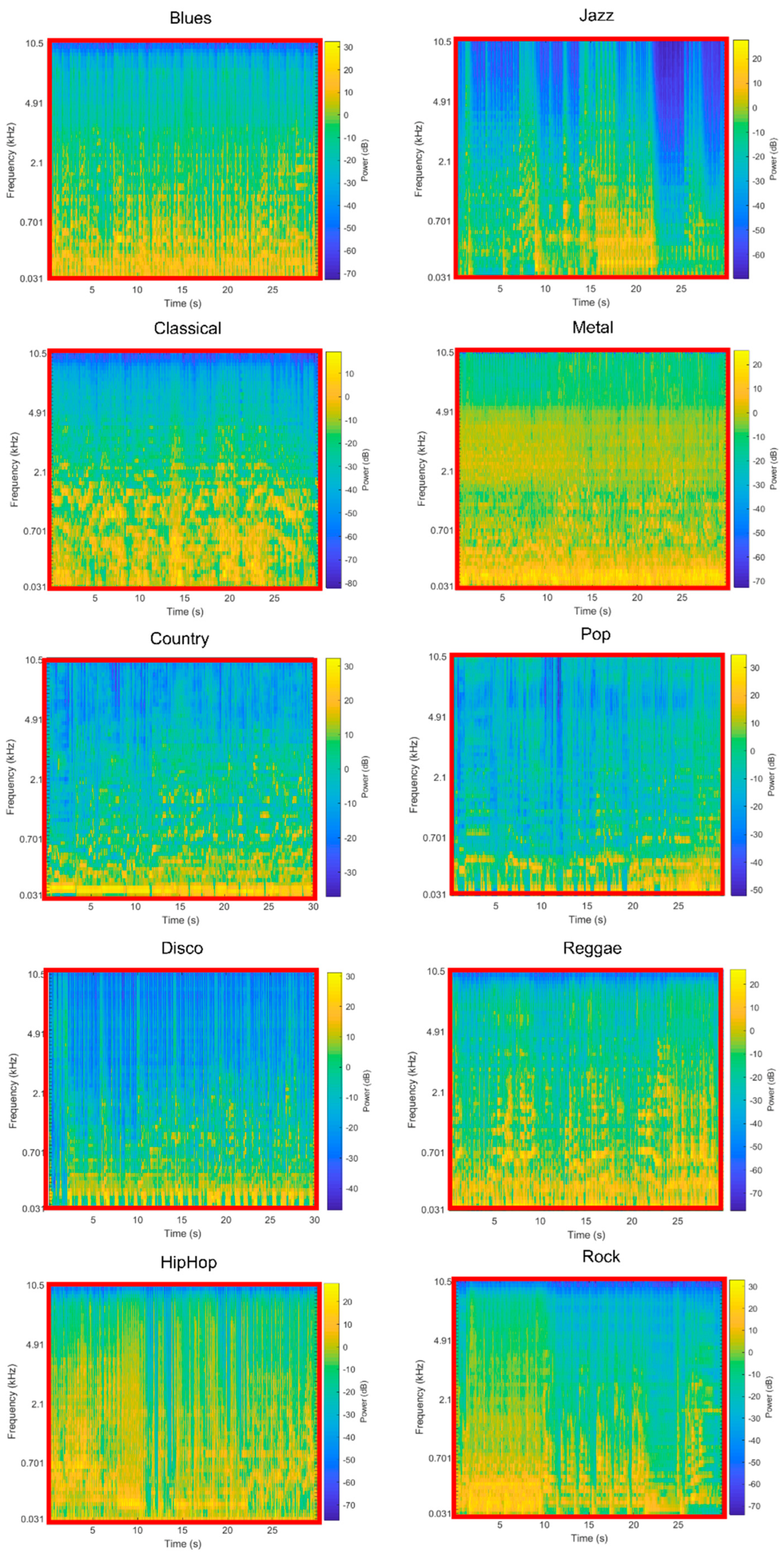
2.1. Definition of Visual Mel Spectrum
2.2. GTZAN Dataset
2.3. Data Preprocessing
2.4. YOLOv4 for Music Genre Classification
2.4.1. Architecture
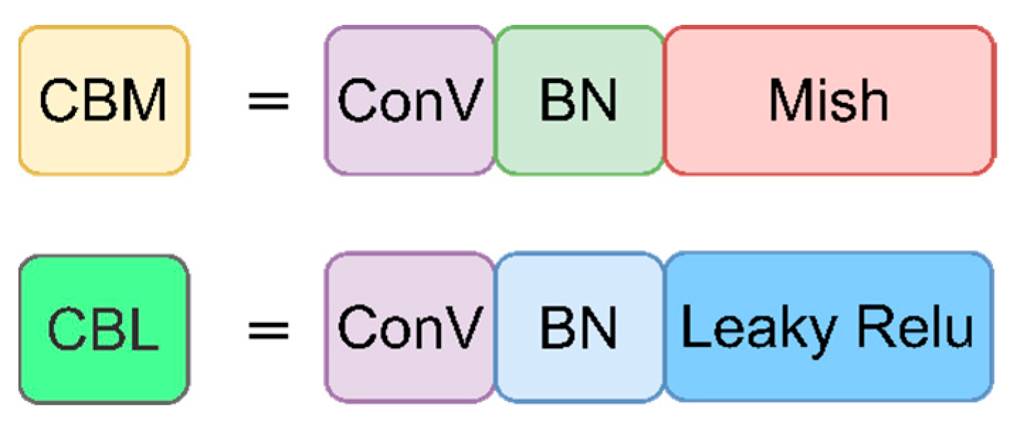
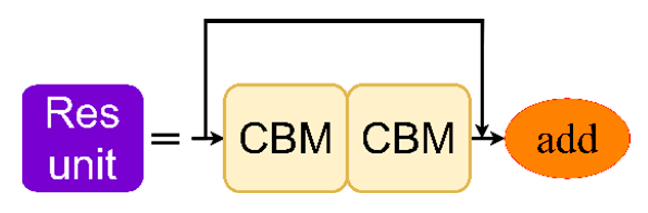
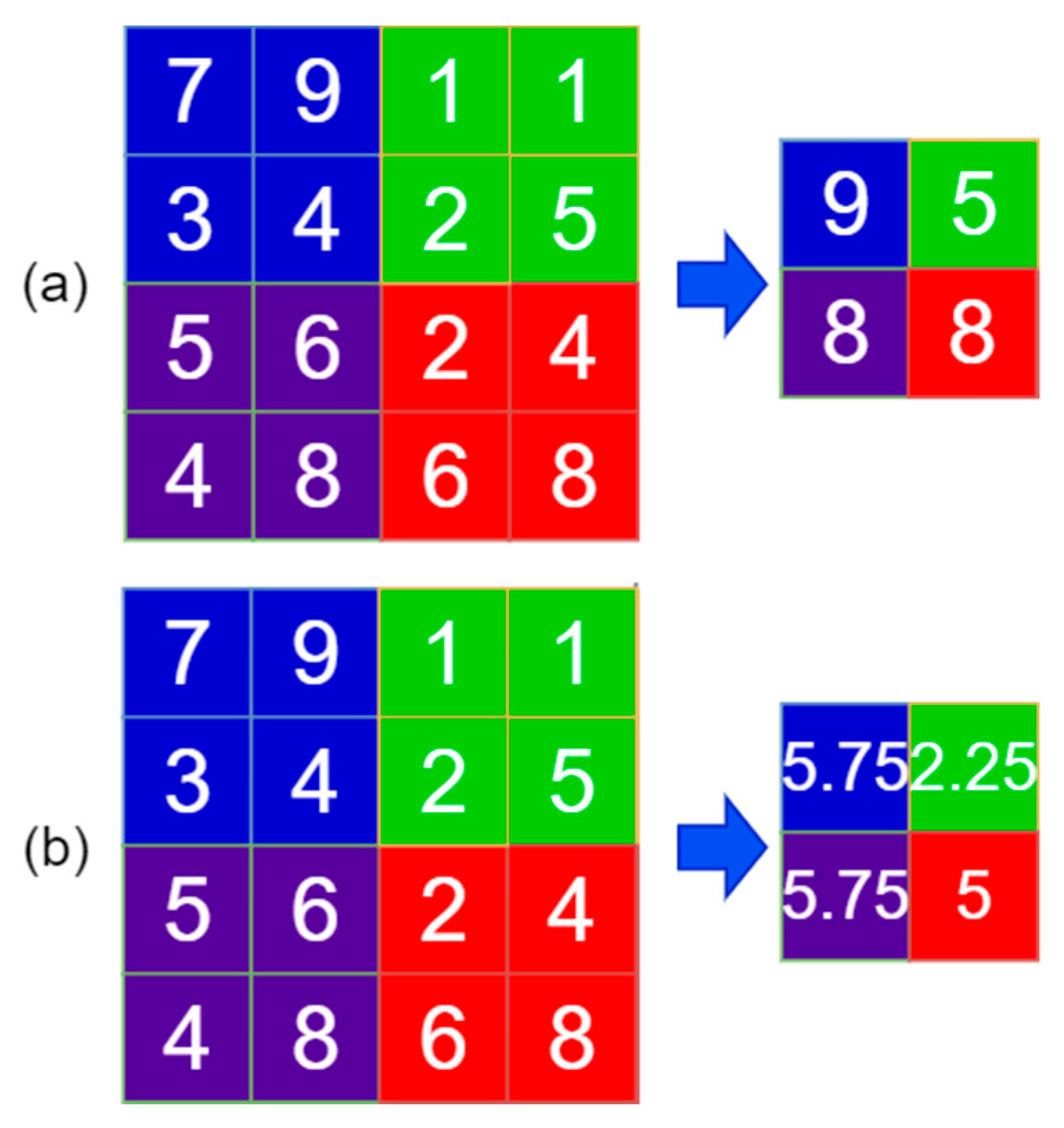
2.4.2. Convolutional Neural Network
2.4.3. Activation Function
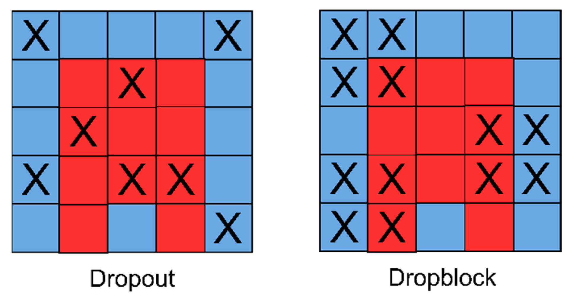
2.4.4. Dropblock
3. Results and Discussion
3.1. Evaluation Criteria
3.2. Parameter Settings for Deep Learning Experiments
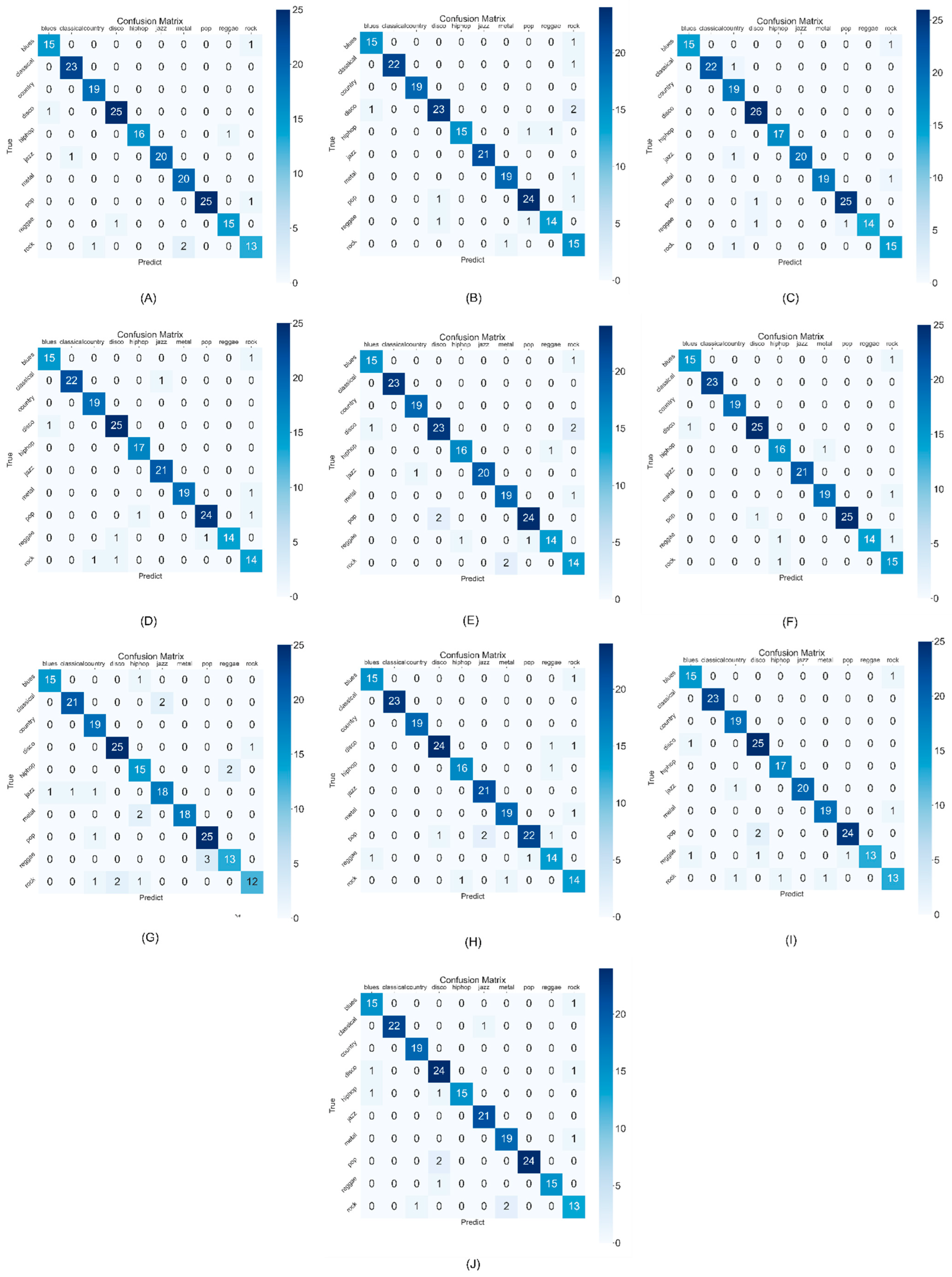
3.3. Results and Analysis
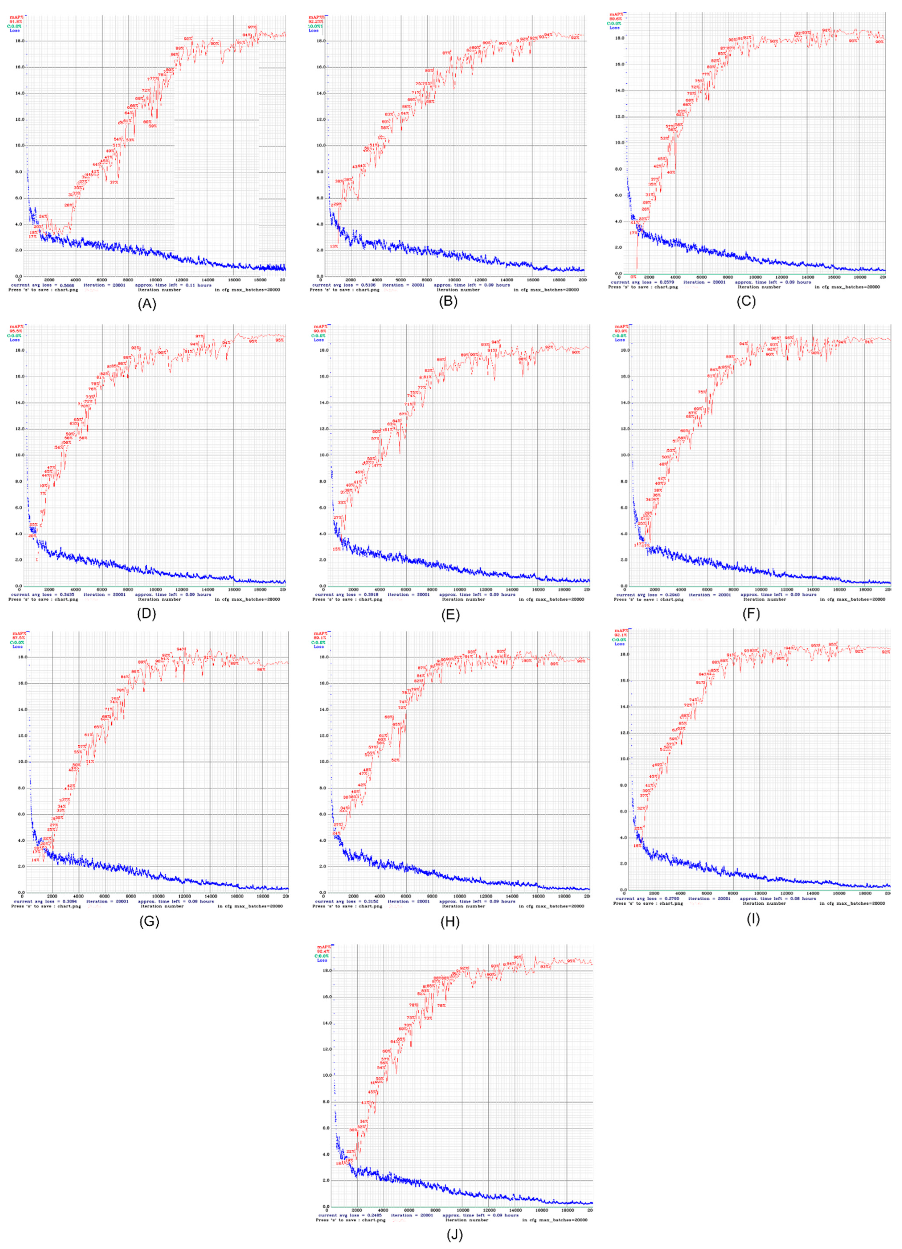
3.4. Test for the Number of Training Sessions
3.5. Comparison of the AVG Accuracy of the Proposed Method with Other Methods
4. Conclusions
- (1)
- Collect representative datasets to verify the accuracy and generalization of this research method.
- (2)
- Integrate several representative datasets to develop a complete visual Mel spectrum dataset for music genre classification.
- (3)
- Investigate other novel deep learning methods to explore the benefits of using the visual Mel spectrum dataset.
- (4)
- Discuss and introduce improvement strategies in music genre classification to promote better performance and results in music classification results.
- (5)
- Develop friendly and available systems for the convenience of music genre classification.
- (1)
- This study proposes the novel visual Mel spectrum, which is different from the traditional Mel spectrum for music genre classification, and is an innovative study.
- (2)
- YOLO has never been used to music genre classification. This study is the first to use YOLO for music genre classification and has research value.
- (3)
- The visual Mel spectrum combined with YOLO achieves higher accuracy compared with other methods, which is a forward-looking method.
Author Contributions
Funding
Institutional Review Board Statement
Informed Consent Statement
Data Availability Statement
Conflicts of Interest
References
- Hillecke, T.; Nickel, A.; Bolay, H.V. Scientific perspectives on music therapy. Ann. N. Y. Acad. Sci. 2005, 1060, 271–282. [Google Scholar] [CrossRef]
- Yehuda, N. Music and stress. J. Adult Dev. 2011, 18, 85–94. [Google Scholar] [CrossRef]
- Thoma, M.V.; La Marca, R.; Brönnimann, R.; Finkel, L.; Ehlert, U.; Nater, U.M. The effect of music on the human stress response. PLoS ONE 2013, 8, e70156. [Google Scholar] [CrossRef] [Green Version]
- Li, T.; Ogihara, M.; Li, Q. A comparative study on content-based music genre classification. In Proceedings of the 26th Annual International ACM SIGIR Conference on Research and Development in Informaion Retrieval, Toronto, ON, Canada, 28 July–1 August 2003; pp. 282–289. [Google Scholar]
- Li, T.; Ogihara, M. Music genre classification with taxonomy. In Proceedings of the IEEE International Conference on Acoustics, Speech, and Signal Processing (ICASSP’05), Philadelphia, PA, USA, 18–23 March 2005; Volume 195, pp. v/197–v/200. [Google Scholar]
- Meng, A.; Ahrendt, P.; Larsen, J.; Hansen, L.K. Temporal feature integration for music genre classification. IEEE Trans. Audio Speech Lang. Process. 2007, 15, 1654–1664. [Google Scholar] [CrossRef] [Green Version]
- Bahuleyan, H. Music genre classification using machine learning techniques. arXiv 2018, arXiv:1804.01149. [Google Scholar]
- Pelchat, N.; Gelowitz, C.M. Neural network music genre classification. Can. J. Electr. Comput. Eng. 2020, 43, 170–173. [Google Scholar] [CrossRef]
- Liu, J.; Wang, C.; Zha, L. A Middle-Level Learning Feature Interaction Method with Deep Learning for Multi-Feature Music Genre Classification. Electronics 2021, 10, 2206. [Google Scholar] [CrossRef]
- Salazar, A.E.C. Hierarchical mining with complex networks for music genre classification. Digit. Signal Process. 2022, 127, 103559. [Google Scholar] [CrossRef]
- Singh, Y.; Biswas, A. Robustness of musical features on deep learning models for music genre classification. Expert Syst. Appl. 2022, 199, 116879. [Google Scholar] [CrossRef]
- Shah, M.; Pujara, N.; Mangaroliya, K.; Gohil, L.; Vyas, T.; Degadwala, S. Music Genre Classification using Deep Learning. In Proceedings of the 2022 6th International Conference on Computing Methodologies and Communication (ICCMC), Erode, India, 29–31 March 2022; pp. 974–978. [Google Scholar]
- Lau, D.S.; Ajoodha, R. Music Genre Classification: A Comparative Study between Deep Learning and Traditional Machine Learning Approaches. In Proceedings of the Sixth International Congress on Information and Communication Technology, London, UK, 25–26 February 2021; pp. 239–247. [Google Scholar]
- Kothari, N.; Kumar, P. Literature Survey for Music Genre Classification Using Neural Network. Int. Res. J. Eng. Technol. 2022, 9, 691–695. [Google Scholar]
- He, Q. A Music Genre Classification Method Based on Deep Learning. Math. Probl. Eng. 2022, 2022, 9668018. [Google Scholar] [CrossRef]
- Qiu, L.; Li, S.; Sung, Y. DBTMPE: Deep bidirectional transformers-based masked predictive encoder approach for music genre classification. Mathematics 2021, 9, 530. [Google Scholar] [CrossRef]
- Allamy, S.; Koerich, A.L. 1D CNN architectures for music genre classification. In Proceedings of the 2021 IEEE Symposium Series on Computational Intelligence (SSCI), Virtual, 5–7 December 2021; pp. 1–7. [Google Scholar]
- Prabhakar, S.K.; Lee, S.-W. Holistic Approaches to Music Genre Classification using Efficient Transfer and Deep Learning Techniques. Expert Syst. Appl. 2023, 211, 118636. [Google Scholar] [CrossRef]
- Davis, S.; Mermelstein, P. Comparison of parametric representations for monosyllabic word recognition in continuously spoken sentences. IEEE Trans. Acoust. Speech Signal Process. 1980, 28, 357–366. [Google Scholar] [CrossRef] [Green Version]
- Tzanetakis, G.; Cook, P. Musical genre classification of audio signals. IEEE Trans. Speech Audio Process. 2002, 10, 293–302. [Google Scholar] [CrossRef]
- Bochkovskiy, A.; Wang, C.-Y.; Liao, H.-Y.M. Yolov4: Optimal speed and accuracy of object detection. arXiv 2020, arXiv:2004.10934. [Google Scholar]
- Misra, D. Mish: A self regularized non-monotonic neural activation function. arXiv 2019, arXiv:1908.08681. [Google Scholar]
- Elbir, A.; Çam, H.B.; Iyican, M.E.; Öztürk, B.; Aydin, N. Music genre classification and recommendation by using machine learning techniques. In Proceedings of the 2018 Innovations in Intelligent Systems and Applications Conference (ASYU), Adana, Turkey, 4–6 October 2018; pp. 1–5. [Google Scholar]
- Rajan, R.; Murthy, H.A. Music genre classification by fusion of modified group delay and melodic features. In Proceedings of the 2017 Twenty-Third National Conference on Communications (NCC), Chennai, India, 2–4 March 2017; pp. 1–6. [Google Scholar]
- Kobayashi, T.; Kubota, A.; Suzuki, Y. Audio feature extraction based on sub-band signal correlations for music genre classification. In Proceedings of the 2018 IEEE International Symposium on Multimedia (ISM), Taichung, Taiwan, 10–12 December 2018; pp. 180–181. [Google Scholar]
- Zheng, E.; Moh, M.; Moh, T.-S. Music genre classification: A n-gram based musicological approach. In Proceedings of the 2017 IEEE 7th International Advance Computing Conference (IACC), Hyderabad, India, 5–7 January 2017; pp. 671–677. [Google Scholar]
- Benetos, E.; Kotropoulos, C. Non-negative tensor factorization applied to music genre classification. IEEE Trans. Audio Speech Lang. Process. 2010, 18, 1955–1967. [Google Scholar] [CrossRef]


| Item | Data |
|---|---|
| Genre | 10 |
| Length | 30 s |
| Sample rate | 22,050 Hz |
| Song mode | Mono |
| Song format | AU |
| Audio files | 16 bits |
| Total | 1000 |
| Parameter | Value |
|---|---|
| Audio Length (seconds) | 30 |
| Window Length (frames) | 1024 |
| Overlap Length (frames) | 512 |
| FFT Length (frames) | 4096 |
| Num Bands (filters) | 64 |
| Model | Mish | Swish | ReLU |
|---|---|---|---|
| Resnet v2-20 | 92.02% | 91.61% | 91.71% |
| WRN 10-2 | 86.83% | 86.56% | 84.56% |
| Simple Net | 91.70% | 91.44% | 91.16% |
| Xception Net | 88.73% | 88.56% | 88.38% |
| Capsule Net | 83.15% | 82.48% | 82.19% |
| Inception ResNet v2 | 85.21% | 84.96% | 82.22% |
| Genre | Number of Songs |
|---|---|
| Blues | 16 |
| Classical | 23 |
| Country | 19 |
| Disco | 26 |
| Hip-hop | 17 |
| Jazz | 21 |
| Metal | 20 |
| Pop | 26 |
| Reggae | 16 |
| Rock | 16 |
| Total | 200 |
| Number of Experiments | mAP of Training | mAP of Testing |
|---|---|---|
| 1 | 91.8% | 94.57% |
| 2 | 92.2% | 96.48% |
| 3 | 89.6% | 97.84% |
| 4 | 95.5% | 98.82% |
| 5 | 90.8% | 98.81% |
| 6 | 93.9% | 98.53% |
| 7 | 87.5% | 99.26% |
| 8 | 89.1% | 97.91% |
| 9 | 92.1% | 98.87% |
| 10 | 92.4% | 98.19% |
| Methods | AVG Accuracy |
|---|---|
| Our method | 94.5% |
| Elbir et al.’s method (Data from [23]) | 72.6% |
| Rajan and Murthy’s method (Data from [24]) | 75.5% |
| Kobayashi et al.s’ method (Data from [25]) | 81.5% |
| Zheng et al.’s method (Data from [26]) | 84.7% |
| Benetos and Kotropoulos’s method (Data from [27]) | 78.9% |
Publisher’s Note: MDPI stays neutral with regard to jurisdictional claims in published maps and institutional affiliations. |
© 2022 by the authors. Licensee MDPI, Basel, Switzerland. This article is an open access article distributed under the terms and conditions of the Creative Commons Attribution (CC BY) license (https://creativecommons.org/licenses/by/4.0/).
Share and Cite
Cheng, Y.-H.; Kuo, C.-N. Machine Learning for Music Genre Classification Using Visual Mel Spectrum. Mathematics 2022, 10, 4427. https://doi.org/10.3390/math10234427
Cheng Y-H, Kuo C-N. Machine Learning for Music Genre Classification Using Visual Mel Spectrum. Mathematics. 2022; 10(23):4427. https://doi.org/10.3390/math10234427
Chicago/Turabian StyleCheng, Yu-Huei, and Che-Nan Kuo. 2022. "Machine Learning for Music Genre Classification Using Visual Mel Spectrum" Mathematics 10, no. 23: 4427. https://doi.org/10.3390/math10234427
APA StyleCheng, Y.-H., & Kuo, C.-N. (2022). Machine Learning for Music Genre Classification Using Visual Mel Spectrum. Mathematics, 10(23), 4427. https://doi.org/10.3390/math10234427