Monitoring Sparse and Attributed Network Streams with MultiLevel and Dynamic Structures

Abstract

In this study, we create a new monitoring system for change detection in sparse attributed network streams with multilevel or nested dynamic structures. To achieve this, we hypothesize that the contingency of establishing an edge between two network nodes at time t depends on the properties of the network edges, network nodes, groups, or categories. Then, we estimate the model parameters using the expressed logit model. The model parameters are developed using the state-space model to achieve a dynamic state in the system. The extended Kalman filter (EKF) updates state-space parameters and predicts upcoming networks. Predicted residuals are tracked using statistical process control charts to identify changes in the underlying mechanism of edge generation. This research makes a methodological contribution by combining zero-inflated generalized linear mixed models (ZI-GLMMs) with the state-space model to monitor changes in the sequences of sparse, attributed, and weighted multilevel networks by applying control charts. The proposed model is compared to previous models to evaluate performance by implementing three scenarios. The results show that the model is faster at detecting the first change. Finally, using real e-MID data, we measured the model’s performance in detecting real data changes. The findings suggest that the proposed model could predict a crisis in advance of significant European Central Bank statements and events.

1. Introduction

Due to the complexity of the real world and the advent of data collection tools, storing information derived from the relationships between elements has become inevitable. A common way to display relationships between elements is by using a network (or graph) in which elements, nodes, and connections represent network edges. For example, in financial markets, we can consider a correlated network of stocks, where each stock is a network node, and the correlation between them is specified by network edges [1]. The supply chain’s resulting network is composed of the links between the various chain components [2]. Communication networks are digital networks [3]. People create the nodes in a social network, and their interactions create the edges [4,5,6,7]. The relationships between people in a social group is an example of a social network [8]. Recent studies have shown a substantial increase in the modeling and analysis of networks in which the connections between network nodes are functions of their characteristics. For example, in a social network, the probability of people communicating depends on their age, gender, and other factors [9]. Azarnoush et al. (2016) modeled the probability of contact between two people using logistic regression [9]. They used subgroup members and correlation data as explanatory variables in their study. Finally, changes in the logistic regression model were detected by the likelihood ratio test appropriate to each new graph. Nonetheless, their method had a drawback; it did not accurately describe network dynamics and dynamic flow. To address this problem, using the generalized linear model (GLM) to model the attributed static network, Gahrooei and Paynabar (2018) developed a statistical method for dynamic social network monitoring [10]. The model was aggregated with the state transfer equation to obtain the dynamic state. They used the Kalman filter to update and predict system parameters over time. In practice, nodes in a network, including networks resulting from financial exchanges between two banks or networks resulting from high correlations between corporate stocks, are sparsely interconnected. Furthermore, GLM is unable to model zero-inflated distributions correctly, because when there are a lot of zeros, the data are difficult to fit into typical distributions (e.g., normal, Poisson, binomial, negative binomial, and beta). As a result, their approach to modeling this type of network is flawed. Ebrahimi S et al. (2021) [11] improved the above-mentioned method based on the Hurdle model to address this problem. They monitored a stream of weighted, attributed, and sparse networks. Modeling sparse networks was their innovation. Using the Hurdle model, this method calculated the probability of edge formation between two nodes. They assessed the validity of their model using two modeling and case study methods. Nonetheless, Their method overlooks the effect of specific variables between groups when predicting the probability of a relationship between the two edges using zero-inflated and Hurdle models. For example, two people living in the same neighborhood communicated more than others in a social network. In the stock market, the correlation of stocks in one category is higher than in other stocks. Likewise, in the interactions between several banks studied by Ebrahimi et al. (2021) [11], the probability of communication and interaction between two banks in the same area or with a common culture was higher than other banks. Data grouping in certain population levels makes using mixed effects models inevitable. Thus, ignoring the fixed and random effects in calculating the likelihood reduces the accuracy of the measurement and increases false results. The use of multilevel networks helps analyze these systems [12,13,14]. Carley reintroduced multilevel network concepts in the analysis of group processes within organizations, in her theory of group stability in 1991 [15]. For example, regarding the application of multilevel networks, Holloway et al. (2016) showed how various micro-mechanisms of multilevel clustering that emerge from the accumulation of mutual and multilateral relationships between countries shape the structure of the global network of fisheries systems [16]. In 2015, the multiplex structure of interbank networks using Italian data was studied by Bargigli et al. [17]. Their findings showed that different layers render several topological and metric properties which are layer specific. Langfield et al. (2014) have analyzed various layers of the U.K. interbank exposure and funding networks using granular U.K. interbank data. They find the importance of considering different layers because structure typically differs among them. According to several empirical studies, network statistics, such as the average network degree distribution, might change depending on whether the market is stable or in a crisis [8]. As far as we know, the obvious approach has not yet been established to routinely detect the new state of these networks in real-time. We fill this gap by improving a method. In this study, we utilize zero-inflated generalized linear mixed models (ZI-GLMM) to develop a method for calculating the probability of a network connection between two nodes by considering their relationship in different levels or groups [18]. As proposed by Courgeau and Franck [19], ZI-GLMM allows the researchers to link observations and contexts such as companies and countries, students and schools, family and neighborhood relationships, and categories. It further considers fixed and random effects in regression. This paper proposes a new method to model and detect changes in sparse, weighted, and attributed network streams with multilevel or nested and dynamic structures. The attributes of nodes and network edges at various network levels described the contingent presence of an edge between two network nodes. Comprehending this process is the main idea of our approach using ZI-GLMM. Sparsity and mixed levels exist in various contexts, including our case study application of financial networks. This study seeks to calculate the probability of creating an edge between two network nodes by taking into account fixed and random effects, as well as other effects in different levels of multilevel networks, which are not considered by the Hurdle model proposed by Ebrahimi et al. [11]. As previously mentioned, fixed effects include factors, such as being a fellow citizen, a teammate, a neighbor, having ethnic relations, and so on. We use the state-space model to achieve a dynamic state and develop the parameters of the ZI-GLMM model over time. Then, the parameters are estimated and updated using the extended Kalman filter (EKF) as an online, recursive inference procedure. Finally, the next step is predicted and compared with the realized network. The network change point is identified and reported using the exponentially weighted moving average (EWMA) control chart to monitor the differences between the two networks. This study makes a methodological contribution by combining ZI-GLMM with the state-space model to monitor changes in the sequences of sparse, attributed, and weighted multilevel networks using control charts. Moreover, the model presented by Ebrahimi et al. [11] is updated by considering the effects of the other network levels when calculating the probability of edge formation between two nodes as previously noted. For this purpose, the proposed method is described in full detail in Section 2. In Section 3, using simulation, we measured the model’s validity and compared it with benchmark methods. Finally, we validated the model using a case study in Section 4.

2. Overview of the Proposed Methodology

This study presents a method for monitoring sparse attributed network streams with multilevel and dynamic structures. This method consists of modeling the network structure and providing a method for detecting changes. The attributes of nodes and network edges at various network levels describe the contingent presence of an edge between two network nodes. For example, the probability of correlation between two stocks in the stock market is a function of the rate of return, grouping, dependency, and other factors. The country of origin’s prevailing interest rate affects the possibility of exchanging between two banks [11]. According to L. P. L. Fávero (2017) [20], there are many situations where data are placed in a mixed or nested structure. Hierarchy refers to the fact that identical observations have similar groups, contexts, aspects, or characteristics, indicating a degree of homogeneity. Although the model presented by Ebrahimi et al. (2021) [11] simulates and monitors sparse attributed network streams with dynamic structures, the proposed Hurdle model cannot model sparse networks with multilevel structures. We used ZI-GLMMs to address this issue [21], and develop the model to simulate sparsely attributed multilevel network streams with dynamic structures. Regular Poisson models are ineffective at simulating zero inflation or deflation, which makes them unsuitable for modeling sparse networks. In this research we assume zero observations have two different origins in our model: “structural” and “sampling". Therefore, a modeling approach that considers all zeros is required. To achieve this goal, we developed the zero-inflated model for dynamic and multilevel settings. Different zero-Inflated models can be introduced but we focus on the “Poisson-logit” specification.

2.1. Zero-Inflated Generalized Linear Mixed Models

Lambert proposed modeling zero-inflated data in 1992 [22]. This model assumes that the data come from a composition of a degenerate distribution at zero and an orderly count distribution, such as the Poison distribution. It is presumed for a zero-inflated Poisson (ZIP) model that for subject i,

$${\mathrm{Y}}_{\mathrm{i}}=\left\{\begin{array}{cc}0\hfill & \mathrm{with}\mathrm{probability}\mathrm{plogi}{\mathrm{t}}_{\mathrm{i}}\hfill \\ \mathrm{Poisson}\left({\mathsf{\lambda }}_{\mathrm{i}}\right)\hfill & \mathrm{with}\mathrm{probability}(1-\mathrm{plogi}{\mathrm{t}}_{\mathrm{i}})\hfill \end{array}\right.$$

(1)

According to the ZIP model, the probability density can be written as follows:

$$\mathrm{P}({\mathrm{Y}}_{\mathrm{i}}=\mathrm{a})=\left\{\begin{array}{cc}\mathrm{plogi}{\mathrm{t}}_{\mathrm{i}}+(1-\mathrm{plogi}{\mathrm{t}}_{\mathrm{i}})\left({\mathrm{e}}^{-{\mathsf{\lambda }}_{\mathrm{i}}}\right)\hfill & \mathrm{i}\mathrm{f}\mathrm{a}=0\hfill \\ (1-\mathrm{plogi}{\mathrm{t}}_{\mathrm{i}})\frac{{\mathsf{\lambda }}_{\mathrm{i}}^{\mathrm{a}}.{\mathrm{e}}^{-{\mathsf{\lambda }}_{\mathrm{i}}}}{\mathrm{a}!}\hfill & \mathrm{i}\mathrm{f}\mathrm{a}>0\hfill \end{array}\right.$$

(2)

Moreover, using the following regressions, the model parameters $\mathrm{plogi}{\mathrm{t}}_{\mathrm{i}}$ and ${\mathsf{\lambda }}_{\mathrm{i}}$ can be estimated by $\mathrm{plogi}{\mathrm{t}}_{\mathrm{i}}={{\mathrm{Z}}_{\mathrm{i}}}^{\mathrm{T}}\mathsf{\delta }$, and, $\ln \left({\mathsf{\lambda }}_{\mathrm{i}}\right)={{\mathrm{X}}_{\mathrm{i}}}^{\mathrm{T}}\mathsf{\pi }$. There are many situations where data are placed in a mixed or nested structure. We used ZI-GLMMs to analyze such data. ZI-GLMMs are versatile and computationally effective models that include elements of generalized linear models, mixed models, and zero-inflated models or similar data. In GLMM, the term mixed-effects refers to the fact that predictor variables can be incorporated in the regression model’s fixed and random effects, with random effects aggregated in the error term. Moreover, as proposed by Courgeau and Franck (2003) [19], ZI-GLMM links observations and contexts, such as companies and countries, students and schools, and family and neighborhood relationships. Furthermore, a multilevel ZIP regression model is developed to handle correlated count data with extra zeros. With this perspective, the two-level zero-inflated count data mixed model is defined as follows:

$$\ln \left(\frac{\mathrm{plogi}{\mathrm{t}}_{\mathrm{ij}}}{1-\mathrm{plogi}{\mathrm{t}}_{\mathrm{ij}}}\right)={{\mathrm{Z}}_{\mathrm{ij}}}^{\mathrm{T}}\mathsf{\delta },\mathrm{being}\mathsf{\delta }={{\mathrm{G}}_{\mathrm{j}}}^{\mathrm{T}}\mathsf{\alpha },$$

(3)

$$\ln \left({\mathsf{\lambda }}_{\mathrm{ij}}\right)={{\mathrm{X}}_{\mathrm{ij}}}^{\mathrm{T}}\mathsf{\pi }+{\mathrm{v}}_{\mathrm{j}},\mathrm{being}\mathsf{\pi }={{\mathrm{L}}_{\mathrm{j}}}^{\mathrm{T}}\mathsf{\beta }$$

The first level refers to observations i (i = 1, 2, 3, …, I). The second level refers to units or layers j (j = 1, 2, 3, …, J). The vectors ${\mathrm{v}}_{\mathrm{j}}$ denote the cluster random effects, Z, X is Matrix of predictor variables and the sentence $\mathsf{\delta }={\mathrm{G}}_{\mathrm{j}}^{\mathrm{T}}\mathsf{\alpha }$ is a regression between j of different levels and $\mathsf{\delta },\mathsf{\alpha },\mathsf{\pi }$ and $\mathsf{\beta }$ are regression parameters. $\mathsf{\delta }$ can be interpreted in terms of the proportion of inflation of zeros, $\mathsf{\pi }$ is related to the mean response in the count data part, and $\mathsf{\alpha }$ and $\mathsf{\beta }$ correspond to the differences among the two contexts in structural and sample zeros, respectively, due to the behavior of predictor variables in level two (${\mathrm{G}}_{\mathrm{j}}$ and ${\mathrm{L}}_{\mathrm{j}}$). Following Lee, Wang, Scott, Yau, and McLachlan (2006) [23] and L. P. L. Fávero, Serra, dos Santos, and Brunaldi (2018) [24], ${\mathsf{\delta }}_{\mathrm{j}}$ represents the random variations at the second level, which means that heterogeneity among higher levels of analyses (groups, for instance) and between individuals is allowed through the random effects $\mathsf{\delta }$, with variance equal to ${\mathsf{\sigma }}_{{\mathrm{v}}_{\mathrm{j}}}^2$. In a network, the set of the observations at time t is equal to the set of the edges between the network nodes in each level and are defined as $\left\{{\mathrm{w}}_{\mathrm{k}\mathrm{d},\mathrm{j},\mathrm{t}}\right|$$\mathrm{k}=1,2,\dots ,\mathrm{K},$$\mathrm{d}=1,2,\dots ,\mathrm{D},$$\mathrm{j}=1,2,\dots ,\mathrm{J},$$\mathrm{t}=1,2,\dots ,\mathrm{T}\}$ That the observation ${\mathrm{w}}_{\mathrm{k}\mathrm{d},\mathrm{j},\mathrm{t}}$ is the weight of the edge between nodes k and d at the j level and at time t; considering ${\mathrm{w}}_{\mathrm{k}\mathrm{d},\mathrm{j},\mathrm{t}}={\mathrm{w}}_{\mathrm{i},\mathrm{j},\mathrm{t}}$, we can say that ${\mathrm{w}}_{\mathrm{k}\mathrm{d},\mathrm{j},\mathrm{t}}$ is the same observation of i at the j level at time t, so:

$$\mathrm{P}({\mathrm{w}}_{\mathrm{k}\mathrm{d},\mathrm{j},\mathrm{t}}=\mathrm{a})=\left\{\begin{array}{cc}\mathrm{plogi}{\mathrm{t}}_{\mathrm{k}\mathrm{d},\mathrm{j},\mathrm{t}}+(1-\mathrm{plogi}{\mathrm{t}}_{\mathrm{k}\mathrm{d},\mathrm{j},\mathrm{t}})\left({\mathrm{e}}^{-{\mathsf{\lambda }}_{\mathrm{k}\mathrm{d},\mathrm{j},\mathrm{t}}}\right)\hfill & \mathrm{i}\mathrm{f}\mathrm{a}=0\hfill \\ (1-\mathrm{plogi}{\mathrm{t}}_{\mathrm{k}\mathrm{d},\mathrm{j},\mathrm{t}})\frac{{{\mathsf{\lambda }}_{\mathrm{k}\mathrm{d},\mathrm{j},\mathrm{t}}}^{\mathrm{a}}.{\mathrm{e}}^{-{\mathsf{\lambda }}_{\mathrm{k}\mathrm{d},\mathrm{j},\mathrm{t}}}}{\mathrm{a}!}\hfill & \mathrm{i}\mathrm{f}\mathrm{a}>0\hfill \end{array}\right.$$

(4)

where $\mathrm{plogi}{\mathrm{t}}_{\mathrm{k}\mathrm{d},\mathrm{j},\mathrm{t}}$ is the probability of the edge between two nodes k, d at the level j and time t. In Equation (4), if $\mathrm{a}>0$ then $\mathrm{P}({\mathrm{w}}_{\mathrm{k}\mathrm{d},\mathrm{j},\mathrm{t}}=\mathrm{a})=(1-\mathrm{plogi}{\mathrm{t}}_{\mathrm{k}\mathrm{d},\mathrm{j},\mathrm{t}})\frac{{{\mathsf{\lambda }}_{\mathrm{k}\mathrm{d},\mathrm{j},\mathrm{t}}}^{\mathrm{a}},{\mathrm{e}}^{-{\mathsf{\lambda }}_{\mathrm{k}\mathrm{d},\mathrm{j},\mathrm{t}}}}{\mathrm{a}!}$, since, a truncated distribution is a conditional distribution that results from restricting the domain of some other probability distribution. Therefore, we consider Equation (4) as follows:

$$\mathrm{P}({\mathrm{w}}_{\mathrm{k}\mathrm{d},\mathrm{j},\mathrm{t}}=\mathrm{a})=\left\{\begin{array}{c}\mathrm{plogi}{\mathrm{t}}_{\mathrm{k}\mathrm{d},\mathrm{j},\mathrm{t}}+(1-\mathrm{plogi}{\mathrm{t}}_{\mathrm{k}\mathrm{d},\mathrm{j},\mathrm{t}})\left({\mathrm{e}}^{-{\mathsf{\lambda }}_{\mathrm{k}\mathrm{d},\mathrm{j},\mathrm{t}}}\right)\mathrm{i}\mathrm{f}\mathrm{a}=0\hfill \\ \mathrm{p}({\mathrm{w}}_{\mathrm{k}\mathrm{d},\mathrm{j},\mathrm{t}}=\mathrm{a}|\mathrm{a}>0)=\frac{\mathrm{p}({\mathrm{w}}_{\mathrm{k}\mathrm{d},\mathrm{j},\mathrm{t}}=(\mathrm{a}\cap \mathrm{a}>0))}{\mathrm{p}({\mathrm{w}}_{\mathrm{k}\mathrm{d},\mathrm{j},\mathrm{t}}=\mathrm{a}>0)}=(1-\mathrm{plogi}{\mathrm{t}}_{\mathrm{k}\mathrm{d},\mathrm{j},\mathrm{t}})\frac{{{\mathsf{\lambda }}_{\mathrm{k}\mathrm{d},\mathrm{j},\mathrm{t}}}^{\mathrm{a}}.{\mathrm{e}}^{-{\mathsf{\lambda }}_{\mathrm{k}\mathrm{d},\mathrm{j},\mathrm{t}}}}{\mathrm{a}!(1-{\mathrm{e}}^{-{\mathsf{\lambda }}_{\mathrm{k}\mathrm{d},\mathrm{j},\mathrm{t}}})}\mathrm{i}\mathrm{f}\mathrm{a}>0\hfill \end{array}\right.$$

(5)

The probabilities of unreported communications are calculated. In a weighted network, if there is no edge between nodes i and j, no weight can be considered for it. Therefore, in specific cases, we can consider Formula (5) as follows:

$$\mathrm{P}({\mathrm{w}}_{\mathrm{k}\mathrm{d},\mathrm{j},\mathrm{t}}=\mathrm{a})=\left\{\begin{array}{c}\mathrm{p}\mathrm{l}\mathrm{o}\mathrm{g}\mathrm{i}{\mathrm{t}}_{\mathrm{k}\mathrm{d},\mathrm{j},\mathrm{t}}\mathrm{i}\mathrm{f}\mathrm{a}=0\hfill \\ (1-\mathrm{p}\mathrm{l}\mathrm{o}\mathrm{g}\mathrm{i}{\mathrm{t}}_{\mathrm{k}\mathrm{d},\mathrm{j},\mathrm{t}})\frac{{{\mathsf{\lambda }}_{\mathrm{k}\mathrm{d},\mathrm{j},\mathrm{t}}}^{\mathrm{a}}.{\mathrm{e}}^{-{\mathsf{\lambda }}_{\mathrm{k}\mathrm{d},\mathrm{j},\mathrm{t}}}}{\mathrm{a}!(1-{\mathrm{e}}^{-{\mathsf{\lambda }}_{\mathrm{k}\mathrm{d},\mathrm{j},\mathrm{t}}})}\mathrm{i}\mathrm{f}\mathrm{a}>0\hfill \end{array}\right.$$

(6)

If $\mathrm{plogi}{\mathrm{t}}_{\mathrm{k}\mathrm{d},\mathrm{j},\mathrm{t}}=0$, clearly the probability distribution of (6) is summarized to the Poisson distribution, if ${\mathrm{w}}_{\mathrm{k}\mathrm{d},\mathrm{j},\mathrm{t}}=0$ will be the Bernoulli probability distribution. In other words, zero observations have two different origins in zero-inflated Poisson regression models, one owing to the binary distribution (structural zeros) and the other owing to the Poisson distribution (sample zeros). To extend the model (6) to a regression setting, we assume that the model parameters $({\mathsf{\lambda }}_{\mathrm{ij}} \mathrm{and} \mathrm{plogi}{\mathrm{t}}_{\mathrm{i}\mathrm{j}})$ are functions of the explanatory variables (node and edge and layer attributes).

$$\ln \left(\frac{\mathrm{p}\mathrm{l}\mathrm{o}\mathrm{g}\mathrm{i}{\mathrm{t}}_{\mathrm{k}\mathrm{d},\mathrm{j},\mathrm{t}}}{1-\mathrm{p}\mathrm{l}\mathrm{o}\mathrm{g}\mathrm{i}{\mathrm{t}}_{\mathrm{k}\mathrm{d}\mathrm{j},\mathrm{t}}}\right)={{\mathrm{Z}}_{\mathrm{k}\mathrm{d},\mathrm{j},\mathrm{t}}}^{\mathrm{T}}\mathsf{\delta },\mathrm{being}\mathsf{\delta }={{\mathrm{G}}_{\mathrm{j},\mathrm{t}}}^{\mathrm{T}}{\mathsf{\beta }}_{0,\mathrm{j},\mathrm{t}},$$

(7)

$$\ln \left({\mathsf{\lambda }}_{\mathrm{k}\mathrm{d},\mathrm{j},\mathrm{t}}\right)={{\mathrm{X}}_{\mathrm{k}\mathrm{d},\mathrm{j},\mathrm{t}}}^{\mathrm{T}}\mathsf{\pi }+{\mathrm{v}}_{\mathrm{j},\mathrm{t}},\mathrm{being}\mathsf{\pi }={{\mathrm{L}}_{\mathrm{j},\mathrm{t}}}^{\mathrm{T}}{\mathsf{\beta }}_{1,\mathrm{j},\mathrm{t}}$$

where, k = 1, 2, 3, …, K, d = 1, 2, 3, …, D, j = 1, 2, 3, …, J, t = 1, 2, 3, …, T and ${\mathrm{Z}}_{\mathrm{k}\mathrm{d},\mathrm{j},\mathrm{t}}^{\mathrm{T}}$ is the transpose matrix of the network edge attributes at the j level and ${\mathrm{G}}_{\mathrm{j},\mathrm{t}}^{\mathrm{T}}$ is the transpose matrix of the characteristics of different surfaces or groups j. The vector ${\mathrm{v}}_{\mathrm{j},\mathrm{t}}$ denotes the cluster or level of random effects. In this step, to obtain the probability value $\mathrm{P}({\mathrm{w}}_{\mathrm{k}\mathrm{d},\mathrm{j},\mathrm{t}}=\mathrm{a})$, we estimate the model parameters. In the manner of Wang, Yau, and Lee (2002) [25], the penalized log-likelihood is given by $\mathrm{l}\mathrm{l}=\mathrm{l}{\mathrm{l}}_1+\mathrm{l}{\mathrm{l}}_2$, with $\mathrm{l}{\mathrm{l}}_1$ being the log-likelihood function when the random effects are conditionally fixed and $\mathrm{l}{\mathrm{l}}_2$ is the log density of the random effects. Lee et al. (2006) [23] present the log-likelihood function for zero-inflated count data mixed models. The first term, $\mathrm{l}{\mathrm{l}}_1$, is given by L. P. L. Fávero (2017) [21] and is related to the ZIP estimations:

$$\mathrm{l}({\mathsf{\beta }}_{0,\mathrm{t}},{\mathsf{\beta }}_{1,\mathrm{t}})=$$

(8)

$$\prod _{{\mathrm{w}}_{\mathrm{k}\mathrm{d},\mathrm{j},\mathrm{t}}=0}\mathrm{plogi}{\mathrm{t}}_{\mathrm{k}\mathrm{d},\mathrm{j},\mathrm{t}}+(1-\mathrm{p}\mathrm{l}\mathrm{o}\mathrm{g}\mathrm{i}{\mathrm{t}}_{\mathrm{k}\mathrm{d},\mathrm{j},\mathrm{t}})\left({\mathrm{e}}^{-{\mathsf{\lambda }}_{\mathrm{k}\mathrm{d},\mathrm{j},\mathrm{t}}}\right)\prod _{\mathrm{w}\mathrm{k}\mathrm{d},\mathrm{j},\mathrm{t}>0}(1-\mathrm{p}\mathrm{l}\mathrm{o}\mathrm{g}\mathrm{i}{\mathrm{t}}_{\mathrm{k}\mathrm{d},\mathrm{j},\mathrm{t}})\frac{{{\mathsf{\lambda }}_{\mathrm{k}\mathrm{d},\mathrm{j},\mathrm{t}}}^{{\mathrm{w}}_{\mathrm{k}\mathrm{d},\mathrm{j},\mathrm{t}}}.{\mathrm{e}}^{-{\mathsf{\lambda }}_{\mathrm{k}\mathrm{d},\mathrm{j},\mathrm{t}}}}{{\mathrm{w}}_{\mathrm{k}\mathrm{d},\mathrm{j},\mathrm{t}}!(1-{\mathrm{e}}^{-{\mathsf{\lambda }}_{\mathrm{k}\mathrm{d},\mathrm{j},\mathrm{t}}})}$$

If N is the total number of outputs and ${\mathrm{N}}_0$ is the total number of zeros in the data, we have:

$$\mathrm{l}({\mathsf{\beta }}_{0,\mathrm{t}},{\mathsf{\beta }}_{1,\mathrm{t}})=$$

(9)

$${[\mathrm{p}\mathrm{l}\mathrm{o}\mathrm{g}\mathrm{i}{\mathrm{t}}_{\mathrm{k}\mathrm{d},\mathrm{j},\mathrm{t}}+(1-\mathrm{p}\mathrm{l}\mathrm{o}\mathrm{g}\mathrm{i}{\mathrm{t}}_{\mathrm{k}\mathrm{d},\mathrm{j},\mathrm{t}})\left({\mathrm{e}}^{-{\mathsf{\lambda }}_{\mathrm{k}\mathrm{d},\mathrm{j},\mathrm{t}}}\right)]}^{{\mathrm{N}}_0}{\left(\frac{1-\mathrm{p}\mathrm{l}\mathrm{o}\mathrm{g}\mathrm{i}{\mathrm{t}}_{\mathrm{k}\mathrm{d},\mathrm{j},\mathrm{t}}}{1-{\mathrm{e}}^{-{\mathsf{\lambda }}_{\mathrm{k}\mathrm{d},\mathrm{j},\mathrm{t}}}}\right)}^{\mathrm{N}-{\mathrm{N}}_0}\prod _{\mathrm{w}\mathrm{k}\mathrm{d},\mathrm{j},\mathrm{t}>0}\frac{{{\mathsf{\lambda }}_{\mathrm{k}\mathrm{d},\mathrm{j},\mathrm{t}}}^{{\mathrm{w}}_{\mathrm{k}\mathrm{d},\mathrm{j},\mathrm{t}}}.{\mathrm{e}}^{-{\mathsf{\lambda }}_{\mathrm{k}\mathrm{d},\mathrm{j},\mathrm{t}}}}{{\mathrm{w}}_{\mathrm{k}\mathrm{d},\mathrm{j},\mathrm{t}}!}$$

Thus, the log-likelihood can be written as follows:

$$\mathrm{l}{\mathrm{l}}_1({\mathsf{\beta }}_{0,\mathrm{t}},{\mathsf{\beta }}_{1,\mathrm{t}})={\mathrm{N}}_0\ln [\mathrm{p}\mathrm{l}\mathrm{o}\mathrm{g}\mathrm{i}{\mathrm{t}}_{\mathrm{k}\mathrm{d},\mathrm{j},\mathrm{t}}+(1-\mathrm{p}\mathrm{l}\mathrm{o}\mathrm{g}\mathrm{i}{\mathrm{t}}_{\mathrm{k}\mathrm{d},\mathrm{j},\mathrm{t}}){\mathrm{e}}^{-{\mathsf{\lambda }}_{\mathrm{k}\mathrm{d},\mathrm{j},\mathrm{t}}}]+$$

$$(\mathrm{N}-{\mathrm{N}}_0)[\mathrm{l}\mathrm{n}(1-\mathrm{p}\mathrm{l}\mathrm{o}\mathrm{g}\mathrm{i}{\mathrm{t}}_{\mathrm{k}\mathrm{d},\mathrm{j},\mathrm{t}})-{\mathsf{\lambda }}_{\mathrm{k}\mathrm{d},\mathrm{j},\mathrm{t}}-\mathrm{l}\mathrm{n}(1-{\mathrm{e}}^{-{\mathsf{\lambda }}_{\mathrm{k}\mathrm{d},\mathrm{j},\mathrm{t}}})]+$$

$$\ln \left({\mathsf{\lambda }}_{\mathrm{k}\mathrm{d},\mathrm{j},\mathrm{t}}\right)\sum _{{\mathrm{w}}_{\mathrm{k}\mathrm{d},\mathrm{j},\mathrm{t}}>0}{\mathrm{w}}_{\mathrm{k}\mathrm{d},\mathrm{j},\mathrm{t}}-\sum _{{\mathrm{w}}_{\mathrm{k}\mathrm{d},\mathrm{j},\mathrm{t}}>0}\ln ({\mathrm{w}}_{\mathrm{k}\mathrm{d},\mathrm{j},\mathrm{t}}!)$$

(10)

and the second term is given by $\mathrm{l}{\mathrm{l}}_2=\frac{-1}{2}[\mathrm{J}\mathrm{l}\mathrm{n}\left(2\mathsf{\pi }{\mathsf{\sigma }}_{\mathrm{v}}^2\right)+{\mathsf{\sigma }}_{\mathrm{v}}^{-2}{\mathrm{v}}^{\mathrm{T}}\mathrm{v}]$. Random effects v allow the existence of heterogeneity among clusters and also among individuals; $\mathrm{l}{\mathrm{l}}_1$ is maximized, and the values of the variance components are updated as a result of the estimation of a restricted maximum likelihood (REML) function from $\mathrm{l}{\mathrm{l}}_2$ [21]. Thus, $\mathrm{l}{\mathrm{l}}_1+\mathrm{l}{\mathrm{l}}_2$ generates the final $\mathrm{l}\mathrm{l}$ for a zero-inflated multilevel model. As stated in Younès, Ezzahid, and Belasri (2012) [26], the numerical algorithm can be used to find the estimated value of ${\mathsf{\lambda }}_{\mathrm{k}\mathrm{d},\mathrm{j},\mathrm{t}}$; by placing ${\mathsf{\lambda }}_{\mathrm{k}\mathrm{d},\mathrm{j},\mathrm{t}}$, the value of $\mathrm{plogi}{\mathrm{t}}_{\mathrm{k}\mathrm{d},\mathrm{j},\mathrm{t}}$ is obtained. In this paper, all estimations are obtained through the software R version 4.1.1. In the next subsection, we will discuss how to incorporate network structural dynamics through a state-space model on the parameters of the ZI-GLMM.

2.2. State Space Models and the Extended Kalman Filter

A state-space model provides a flexible framework to represent linear or generally non-linear dynamic models. The system’s state is unknown in general, but it can be deduced using the observation method. Therefore, we assume that $\mathsf{\beta }=({\mathsf{\beta }}_{0,\mathrm{t}},{\mathsf{\beta }}_{1,\mathrm{t}})$, (coefficients specified in Equation (7)), are system state variables, which are driven by a random process, and observations of network edges ${\mathrm{w}}_{\mathrm{k}\mathrm{d},\mathrm{j},\mathrm{t}}$, t = 1, 2, …, T are considered noisy observations. Thus, according to Ebrahimi et al. (2021) [11], we consider the state-space model as follows:

$${\mathsf{\beta }}_{\mathrm{j},\mathrm{t}}=\mathrm{F}\mathsf{\beta }\mathrm{j},\mathrm{t}-1+{\mathsf{ϵ}}_{\mathrm{j},\mathrm{t}}$$

(11)

$${\mathrm{w}}_{\mathrm{k}\mathrm{d},\mathrm{j},\mathrm{t}}=\mathrm{W}({\mathrm{Z}}_{\mathrm{k}\mathrm{d},\mathrm{j},\mathrm{t}},{\mathrm{X}}_{\mathrm{k}\mathrm{d},\mathrm{j},\mathrm{t}},{\mathrm{G}}_{\mathrm{j},\mathrm{t}},{\mathrm{L}}_{\mathrm{j},\mathrm{t}},{\mathsf{\beta }}_{\mathrm{j},\mathrm{t}})$$

where ${\mathsf{\beta }}_{,\mathrm{j},\mathrm{t}}=({\mathsf{\beta }}_{0,\mathrm{j},\mathrm{t}},{\mathsf{\beta }}_{1,\mathrm{j},\mathrm{t}})$ is the state vector and F is the state transfer matrix, the error term ${\mathsf{ϵ}}_{\mathrm{t}}\sim \mathcal{N}(0,{\mathrm{Q}}_{\mathrm{t}})$ has a normal distribution with zero mean and variance ${\mathrm{Q}}_{\mathrm{t}}$. ${\mathrm{X}}_{\mathrm{k}\mathrm{d},\mathrm{j},\mathrm{t}},{\mathrm{Z}}_{\mathrm{k}\mathrm{d},\mathrm{j},\mathrm{t}}$, respectively, are the attributes of node k ending in node d, and the edge attributes between node k and d in layer j and ${\mathrm{G}}_{\mathrm{j},\mathrm{t}}$,${\mathrm{L}}_{\mathrm{j},\mathrm{t}}$ are the attributes of layer j at time t. W is a nonlinear link function that with data $({\mathrm{Z}}_{\mathrm{k}\mathrm{d},\mathrm{j},\mathrm{t}},{\mathrm{X}}_{\mathrm{k}\mathrm{d},\mathrm{j},\mathrm{t}},{\mathrm{G}}_{\mathrm{j},\mathrm{t}},{\mathrm{L}}_{\mathrm{j},\mathrm{t}},{\mathsf{\beta }}_{,\mathrm{j},\mathrm{t}})$ Provides a proper understanding of ${\mathrm{w}}_{\mathrm{k}\mathrm{d},\mathrm{j},\mathrm{t}}$. The $\mathrm{l}\mathrm{l}$ function can be divided into two parts, with the most significant value of the total obtained by maximizing each component separately. As a result, we consider the W function as follows:

$$\mathrm{W}({\mathrm{Z}}_{\mathrm{k}\mathrm{d},\mathrm{j},\mathrm{t}},{\mathrm{X}}_{\mathrm{k}\mathrm{d},\mathrm{j},\mathrm{t}},{\mathrm{G}}_{\mathrm{j},\mathrm{t}},{\mathrm{L}}_{\mathrm{j},\mathrm{t}},{\mathsf{\beta }}_{,\mathrm{j},\mathrm{t}})\left\{\begin{array}{c}\frac{{\mathrm{e}}^{{\mathrm{Z}}_{\mathrm{k}\mathrm{d},\mathrm{j},\mathrm{t}}^{\mathrm{T}}\mathsf{\delta }}}{1+{\mathrm{e}}^{{\mathrm{Z}}_{\mathrm{k}\mathrm{d},\mathrm{j},\mathrm{t}}^{\mathrm{T}}\mathsf{\delta }}},\mathsf{\delta }={\mathrm{G}}_{\mathrm{j},\mathrm{t}}^{\mathrm{T}}{\mathsf{\beta }}_{0,\mathrm{j},\mathrm{t}}\mathrm{f}\mathrm{o}\mathrm{r}\mathrm{m}\mathrm{o}\mathrm{d}\mathrm{e}\mathrm{l}\mathrm{i}\mathrm{n}\mathrm{g}\mathrm{t}\mathrm{h}\mathrm{e}\mathrm{z}\mathrm{e}\mathrm{r}\mathrm{o}\mathrm{c}\mathrm{o}\mathrm{u}\mathrm{n}\mathrm{t}\mathrm{s}\hfill \\ {\mathrm{e}}^{{\mathrm{X}}_{\mathrm{k}\mathrm{d},\mathrm{j},\mathrm{t}}^{\mathrm{T}}\mathsf{\pi }+{\mathrm{v}}_{\mathrm{j},\mathrm{t}}},\mathsf{\pi }={\mathrm{L}}_{\mathrm{j},\mathrm{t}}^{\mathrm{T}}{\mathsf{\beta }}_{1,\mathrm{j},\mathrm{t}}\mathrm{f}\mathrm{o}\mathrm{r}\mathrm{n}\mathrm{o}\mathrm{n}\mathrm{z}\mathrm{e}\mathrm{r}\mathrm{o}\hfill \end{array}\right.$$

(12)

${\mathsf{\beta }}_{1,\mathrm{j},\mathrm{t}}$ and ${\mathsf{\beta }}_{0,\mathrm{j},\mathrm{t}}$ are the estimated regression coefficients at time t. Thus far, we have estimated the values and defined a state-space model for it. The next step is to estimate the model parameters and update them using the EKF. Although the EKF was designed for observations with a normal distribution, Fahrmeir L, Kaufmann H in 1991 demonstrated that it may also be utilized for the exponential distribution family. Therefore, it can be used for the proposed model. Brown and Hwang (1997) [27] explain the prediction and update the equations for EKF.

Assume that ${\mathsf{\beta }}_{\mathrm{t}|\mathrm{t}-1}$ is the prediction of the state of ${\mathsf{\beta }}_{\mathrm{t}}$ and ${\mathrm{P}}_{\mathrm{t}|\mathrm{t}-1}$ is the covariance matrix of the observations up to $\mathrm{t}-1$ and ${\mathsf{\beta }}_{\mathrm{t}|\mathrm{t}}$, and ${\mathrm{P}}_{\mathrm{t}|\mathrm{t}}$ represent the estimation of the state variable and the covariance matrix up to time t. Therefore, the prediction equations at time t will be as follows [11]:

$${\mathsf{\beta }}_{\mathrm{t}|\mathrm{t}-1}=\mathrm{F}{\mathsf{\beta }}_{\mathrm{t}-1|\mathrm{t}-1}$$

$${\mathrm{p}}_{\mathrm{t}|\mathrm{t}-1}=\mathrm{F}{\mathsf{\beta }}_{\mathrm{t}-1|\mathrm{t}-1}{\mathrm{F}}^{\mathrm{T}}+\mathrm{Q},\mathrm{t}=1,2,\dots$$

(13)

The ${\mathsf{\beta }}_{0|0}$ and ${\mathrm{P}}_{0|0}$ can be estimated by fitting the model on the data obtained from the first snapshot of the network. If ${\mathrm{w}}_{\mathrm{t}}=\mathrm{v}\mathrm{e}\mathrm{c}\left[{\mathrm{w}}_{\mathrm{k}\mathrm{d},\mathrm{j},\mathrm{t}}\right]$ is a vectorized adjacency matrix of the network resulting from exchanges between the network nodes and vector ${\mathrm{Z}}_{\mathrm{t}}$, ${\mathrm{G}}_{\mathrm{t}}$ contains j components of ${\mathrm{Z}}_{\mathrm{k}\mathrm{d},\mathrm{j},\mathrm{t}}$ and ${\mathrm{G}}_{\mathrm{j},\mathrm{t}}$, and vectors ${\mathrm{X}}_{\mathrm{t}}$ and ${\mathrm{L}}_{\mathrm{t}}$ contain the j vectors ${\mathrm{X}}_{\mathrm{k}\mathrm{d},\mathrm{j},\mathrm{t}}{\mathrm{L}}_{\mathrm{j},\mathrm{t}}$ in time t, the incoming network data $\left({\mathrm{w}}_{\mathrm{t}}\right)$ are used to update the predicted parameters using the following equations:

$${\mathrm{k}}_{\mathrm{t}}={\mathrm{P}}_{{\mathrm{t}}_{\mathrm{t}}-1}{\mathrm{H}}_{\mathrm{t}}^{\mathrm{T}}{({\mathrm{H}}_{\mathrm{t}}{\mathrm{P}}_{\mathrm{t}|\mathrm{t}-1}{\mathrm{H}}_{\mathrm{t}}^{\mathrm{T}}+{\mathrm{R}}_{\mathrm{t}})}^{-1}$$

(14)

$$\mathsf{\beta }={\mathsf{\beta }}_{\mathrm{t}|\mathrm{t}-1}+{\mathrm{k}}_{\mathrm{t}}({\mathrm{w}}_{\mathrm{t}}-\mathrm{W}({\mathrm{Z}}_{\mathrm{t}},{\mathrm{X}}_{\mathrm{t}},{\mathrm{G}}_{\mathrm{t}},{\mathrm{L}}_{\mathrm{t}},{\mathsf{\beta }}_{\mathrm{t}|\mathrm{t}-1}))$$

$${\mathrm{p}}_{\mathrm{t}|\mathrm{t}}=(\mathrm{I}-{\mathrm{k}}_{\mathrm{t}}{\mathrm{H}}_{\mathrm{t}}){\mathrm{P}}_{\mathrm{t}|\mathrm{t}-1}$$

where ${\mathrm{H}}_{\mathrm{t}}={\left[\frac{\mathrm{d}\mathrm{W}}{\mathrm{d}\mathsf{\beta }}\right]}_{\mathsf{\beta }={\mathsf{\beta }}_{\mathrm{t}|\mathrm{t}}}$ is the measurement Jacobian matrix used for the linearization of the observation function. $\mathrm{W}({\mathrm{Z}}_{\mathrm{k}\mathrm{h},\mathrm{j},\mathrm{t}},{\mathrm{X}}_{\mathrm{k}\mathrm{h},\mathrm{j},\mathrm{t}},{\mathrm{G}}_{\mathrm{j},\mathrm{t}},{\mathrm{L}}_{\mathrm{j},\mathrm{t}},\mathsf{\beta })$, ${\mathrm{K}}_{\mathrm{t}}$ are known as the Kalman gain, ${\mathrm{R}}_{\mathrm{t}}$ is a covariance matrix of the observation at time t, which depends on the distribution of observations for Bernoulli observations ${\mathrm{R}}_{\mathrm{i},\mathrm{j},\mathrm{t}}=(1-{\widehat{\mathrm{p}\mathrm{l}\mathrm{o}\mathrm{g}\mathrm{i}\mathrm{t}}}_{\mathrm{i},\mathrm{j},\mathrm{t}}){\widehat{\mathsf{\lambda }}}_{\mathrm{i},\mathrm{j},\mathrm{t}}$; the positive Poisson is equal to ${\mathrm{R}}_{\mathrm{i},\mathrm{j},\mathrm{t}}=\frac{{\widehat{\mathsf{\lambda }}}_{\mathrm{i},\mathrm{j},\mathrm{t}}}{1-exp(-{\widehat{\mathsf{\lambda }}}_{\mathrm{i},\mathrm{j},\mathrm{t}})}(1+{\widehat{\mathsf{\lambda }}}_{\mathrm{i},\mathrm{j},\mathrm{t}}+\frac{{\widehat{\mathsf{\lambda }}}_{\mathrm{i},\mathrm{j},\mathrm{t}}}{1-exp(-{\widehat{\mathsf{\lambda }}}_{\mathrm{i},\mathrm{j},\mathrm{t}})})$ Because the initial values of the F and Q matrices are unknown, we first estimate the initial values for each network in control, ${\mathrm{w}}_{\mathrm{t}}$. Using the multi-dimensional time-series representation and a vector auto-regression (VAR) model, we estimate the initial values ${\mathrm{F}}_0$ and ${\mathrm{Q}}_0$ for the Bernoulli model and ${\mathrm{F}}_1$ and ${\mathrm{Q}}_1$ for the positive Poisson model [11]. After the initialization of F and Q matrices, the process of updating and predicting $\mathsf{\beta }$ matrix values using the state-space model and Kalman filter will be performed, and the ${\mathrm{w}}_{\mathrm{t}}$ network is predicted using the obtained values. In the next section, we use the EWMA control chart to monitor the multilevel sparse network stream changes.

2.3. Monitoring of Dynamic and Multilevel Sparse Network Streams

Prediction residuals are tracked by statistical process control charts in this part in order to identify changes in the underlying mechanism of edge generation. For this purpose, the adjacency matrix obtained from the predicted values is compared with the adjacency matrix obtained from real values. $({\widehat{\mathrm{\epsilon }}}_{\mathrm{k},\mathrm{d},\mathrm{t}}={\mathrm{w}}_{\mathrm{k},\mathrm{d},\mathrm{t}}-{\widehat{\mathrm{w}}}_{\mathrm{k},\mathrm{d},\mathrm{t}})$. To ensure the residuals have approximately constant unit variances, we used the Pearson residuals, denoted by ${\mathrm{r}}_{\mathrm{k},\mathrm{d},\mathrm{t}}$, computed by ${\mathrm{r}}_{\mathrm{k},\mathrm{d},\mathrm{t}}=\frac{{\widehat{\mathrm{\epsilon }}}_{\mathrm{k},\mathrm{d},\mathrm{t}}}{\sqrt{\mathrm{v}\mathrm{a}\mathrm{r}\left({\widehat{\mathrm{w}}}_{\mathrm{k},\mathrm{d},\mathrm{t}}\right)}}$; for $\mathrm{t}=1,2,\dots ,\mathrm{T}$. Instead of monitoring any value of ${\mathrm{r}}_{\mathrm{k},\mathrm{d},\mathrm{t}}$, the values of ${\overline{\mathrm{r}}}_{\mathrm{t}}=\frac{1}{\mathrm{K}}{\sum }_{\mathrm{k},\mathrm{d}}{\mathrm{r}}_{\mathrm{k},\mathrm{d},\mathrm{t}}$ that have normal distributions are monitored using the EWMA control chart [11]. The EWMA statistic at time t is calculated with ${\mathrm{\omega }}_{\mathrm{t}}=\mathsf{\lambda }{\overline{\mathrm{r}}}_{\mathrm{t}+1}+(1-\mathsf{\lambda }){\mathrm{\omega }}_{\mathrm{t}-1}$, and the upper and lower bounds of the EWMA control chart at time t are calculated by $\mathrm{U}\mathrm{C}{\mathrm{L}}_{\mathrm{t}}=\mathcal{L}\times \mathrm{s}\sqrt{\frac{\mathsf{\lambda }}{1-\mathsf{\lambda }}(1-{(1-\mathsf{\lambda })}^{2\mathrm{t}})}$ and $\mathrm{L}\mathrm{C}{\mathrm{L}}_{\mathrm{t}}=-\mathcal{L}\times \mathrm{s}\sqrt{\frac{\mathsf{\lambda }}{1-\mathsf{\lambda }}(1-{(1-\mathsf{\lambda })}^{2\mathrm{t}})}$ that $\mathsf{\lambda }\in [0,1]$. ($\mathcal{L}$ is the multiple of the rational subgroup standard deviation that establishes the control limits. $\mathcal{L}$ is typically set at 3 to match the other control charts, but it may be necessary to reduce $\mathcal{L}$ slightly for small values of $\mathsf{\lambda }$). If $\mathrm{U}\mathrm{C}{\mathrm{L}}_{\mathrm{T}+1}\le {\mathrm{\omega }}_{\mathrm{T}+1}$ or $\mathrm{L}\mathrm{C}{\mathrm{L}}_{\mathrm{T}+1}\ge {\mathrm{\omega }}_{\mathrm{T}+1}$, the null hypothesis that there is a change in the network stream is rejected.

3. Performance Evaluation Using Simulation

This section evaluates the proposed model compared to the online Hurdle model [11] using a simulation to examine the speed of detecting changes in the model. (The proposed model in [11] has already been compared with “Dynamic GLM”, “Dynamic Average Weight”, and ”Degree and Betweenness-EWMA” models, and its advantage has been reported). For this purpose, to more closely match the actual data settings in terms of network size and the number of explanatory auxiliary variables, we consider a network with 50 nodes and a potential of $50\times (50-1)=2450$ edges. We assume that the weight of each edge at each level $(\mathrm{j}=2)$ is a function of five attributes ${\mathrm{Z}}_{\mathrm{k}\mathrm{d},\mathrm{j},\mathrm{t}}={\mathrm{X}}_{\mathrm{k}\mathrm{d},\mathrm{j},\mathrm{t}}=\left\{{\mathrm{X}}_{\mathrm{k}\mathrm{d},\mathrm{j},\mathrm{t}}^1,{\mathrm{X}}_{\mathrm{k}\mathrm{d},\mathrm{j},\mathrm{t}}^2,{\mathrm{X}}_{\mathrm{k}\mathrm{d},\mathrm{j},\mathrm{t}}^3,{\mathrm{X}}_{\mathrm{k}\mathrm{d},\mathrm{j},\mathrm{t}}^4,{\mathrm{X}}_{\mathrm{k}\mathrm{d},\mathrm{j},\mathrm{t}}^5\right\}$, where each ${\mathrm{X}}_{\mathrm{k}\mathrm{d},\mathrm{j},\mathrm{t}}^{\mathrm{e}}=\left\{{\mathrm{X}}_{\mathrm{k}\mathrm{d},1,\mathrm{t}}^{\mathrm{e}},{\mathrm{X}}_{\mathrm{k}\mathrm{d},2,\mathrm{t}}^{\mathrm{e}}\right\}$, $\mathrm{e}=1,2,3,4,5$, $\mathrm{j}=1,2$, and the attribute of each level is ${\mathrm{G}}_{\mathrm{j},\mathrm{t}}={\mathrm{L}}_{\mathrm{j},\mathrm{t}}=\left\{{\mathrm{G}}_{1,\mathrm{t}},{\mathrm{G}}_{2,\mathrm{t}}\right\}$. The attribute value changes over time and is different for each edge and level. It is also created using a normal distribution with mean $\mathsf{\mu }=[0.5,0.5,0,5,0,5,0,5]$ and variance $\sum =0.25\times {\mathrm{I}}_{5\times 5}$ for the edges and mean $\mathsf{\mu }=[0.5,0.5]$ and variance $\sum =0.25\times {\mathrm{I}}_{2\times 2}$ for levels. To simulate a dynamic stream of networks, we assume ${\mathsf{\beta }}_{0,\mathrm{t}}=\mathrm{F}{\mathsf{\beta }}_{0,\mathrm{t}-1}+{\mathsf{ϵ}}_{0,\mathrm{t}},$${\mathsf{\beta }}_{1,\mathrm{t}}=\mathrm{F}{\mathsf{\beta }}_{1,\mathrm{t}-1}+{\mathsf{ϵ}}_{1,\mathrm{t}}$ that ${\mathsf{ϵ}}_{0,\mathrm{t}}\sim \mathcal{N}(0,\mathrm{Q}),$${\mathsf{ϵ}}_{1,\mathrm{t}}\sim \mathcal{N}(0,\mathrm{Q})$. In the simulations, the Values ${\mathsf{\beta }}_{0,\mathrm{t}}=\left\{{\mathsf{\beta }}_{0,\mathrm{t}}^0,{\mathsf{\beta }}_{0,\mathrm{t}}^1,{\mathsf{\beta }}_{0,\mathrm{t}}^2,{\mathsf{\beta }}_{0,\mathrm{t}}^3,{\mathsf{\beta }}_{0,\mathrm{t}}^4,{\mathsf{\beta }}_{0,\mathrm{t}}^5\right\}$ and ${\mathsf{\beta }}_{1,\mathrm{t}}=\left\{{\mathsf{\beta }}_{1,\mathrm{t}}^0,{\mathsf{\beta }}_{1,\mathrm{t}}^1,{\mathsf{\beta }}_{1,\mathrm{t}}^2,{\mathsf{\beta }}_{1,\mathrm{t}}^3,{\mathsf{\beta }}_{1,\mathrm{t}}^4,{\mathsf{\beta }}_{1,\mathrm{t}}^5\right\}$ at $\mathrm{t}=0$ are considered equal ${\mathsf{\beta }}_{0,\mathrm{t}}=\left\{0.01,0.01,0.01,0.01,0.01,0.01\right\}$, and ${\mathsf{\beta }}_{1,\mathrm{t}}=\left\{0.02,0.02,0.02,0.02,0.02,0.02\right\}$, and $\mathrm{F}=0.8{\mathrm{I}}_{6\mathrm{\times }6}$, $\mathrm{Q}=0.25{\mathrm{I}}_{6\mathrm{\times }6}$.

Random effects ${\mathrm{v}}_{\mathrm{j},\mathrm{t}}$ have a normal bivariate distribution with a mean of 0 and covariance $\sum =\left[\begin{array}{cc}{\sum }_{11}& 0\\ 0& {\sum }_{22}\end{array}\right]$ where the ∑ is the estimate of the model parameters. (For model comparability, we identically use the simulation settings from [11]. We estimate the control chart and determine the EWMA control limits using in-control simulated snapshots of networks using the techniques outlined in Section 2.3. In order to evaluate the performance of the proposed model and compare it with the online Hurdle model, we consider three scenarios in two modes [11]. Moreover, the method’s performance is evaluated with the average run length (ARL), which shows the speed detection of changes in each scenario for different values of $\mathsf{\delta }$. For this, we created a network simulation for an out-of-control scenario, with the first out-of-control alarm sounding. Then, we record the number of simulated points until the first change occurs (ARL). We do this process 1000 times and record the average run length. The method with the smallest ARL is more effective at detecting changes. In Equation (13), F is the model coefficient matrix, and Q is the model error covariance matrix. In order to execute the scenarios, for each coefficient ${\mathsf{\beta }}_{\mathrm{i}}$, we consider the shift value $\mathsf{\delta }{\mathsf{\sigma }}_{\mathrm{i}}$. The value of $\mathsf{\delta }$ represents the magnitude of the shift and ${\mathsf{\sigma }}_{\mathrm{i}}$ is the standard deviation of the ith factor in the controlled position. Given the initial values of F and Q, ${\mathsf{\sigma }}_{\mathrm{I}}=\sqrt{\frac{{\mathrm{Q}}_{\mathrm{i}\mathrm{i}}}{{(1-{\mathrm{F}}_{\mathrm{i}\mathrm{i}})}^2)}}=2.5$ so ${{\mathsf{\beta }}^{\mathrm{i}}}_{0,\mathrm{t}}={\mathrm{F}}_{\mathrm{i}\mathrm{i}}{{\mathsf{\beta }}^{\mathrm{i}}}_{0,\mathrm{t}-1}+{{\mathsf{ϵ}}^{\mathrm{i}}}_{0,\mathrm{t}}+\mathsf{\delta }{\mathsf{\sigma }}_{\mathrm{i}}$ and ${{\mathsf{\beta }}^{\mathrm{i}}}_{1,\mathrm{t}}={\mathrm{F}}_{\mathrm{i}\mathrm{i}}{{\mathsf{\beta }}^{\mathrm{i}}}_{1,\mathrm{t}-1}+{{\mathsf{ϵ}}^{\mathrm{i}}}_{1,\mathrm{t}}+\mathsf{\delta }{\mathsf{\sigma }}_{\mathrm{i}}$. If the value of the coefficients ${\mathsf{\beta }}_{0,\mathrm{t}}^{\mathrm{i}}$ changes, it affects the presence or absence of edges between two network nodes. If the value of the coefficients ${{\mathsf{\beta }}^{\mathrm{i}}}_{1,\mathrm{t}}$ changes, it will affect the edge weight. Therefore, to the first scenario, to investigate the presence or absence of edges between the two nodes of the network as well as changes in the weight of the network edges over time, we apply the change value of three coefficients ${{\mathsf{\beta }}^2}_{0,\mathrm{t}}$, ${{\mathsf{\beta }}^4}_{0,\mathrm{t}}$, ${{\mathsf{\beta }}^5}_{0,\mathrm{t}}$, and ${{\mathsf{\beta }}^2}_{1,\mathrm{t}}$, ${{\mathsf{\beta }}^4}_{1,\mathrm{t}}$, ${{\mathsf{\beta }}^5}_{1,\mathrm{t}}$, and the results for two modes $\left\{{\mathrm{G}}_{1,\mathrm{t}}=1,{\mathrm{G}}_{2,\mathrm{t}}=1\right\}$ and $\left\{{\mathrm{G}}_{1,\mathrm{t}}={\mathrm{H}}_{1,\mathrm{t}},{\mathrm{G}}_{2,\mathrm{t}}={\mathrm{H}}_{2,\mathrm{t}}\right\}$, are compared with the results of [11]. In the second scenario, in order to investigate the changes in the relationship between the nodes, we just change the values in three coefficients ${\mathsf{\beta }}_{0,\mathrm{t}}^2,{\mathsf{\beta }}_{0,\mathrm{t}}^4,{\mathsf{\beta }}_{0,\mathrm{t}}^5$. By applying the change values in three coefficients ${\mathsf{\beta }}_{1,\mathrm{t}}^2,{\mathsf{\beta }}_{1,\mathrm{t}}^4,{\mathsf{\beta }}_{1,\mathrm{t}}^5$ in scenario 3, the effect of the change is only on the amount of the interaction (edge weight) between the two nodes. By defining the control limits, we use adjusted control limits for detection in the out of control scenarios. (the in-control ARL for all methods is equal to 200 $(\mathsf{\alpha }=0.005)$). In order to influence the level attributes in the Hurdle model, the following approach was used:

$${\mathrm{Z}}_{\mathrm{k}\mathrm{d},\mathrm{j},\mathrm{t}\left(\mathrm{n}\mathrm{e}\mathrm{w}\right)}^{\mathrm{T}}={\mathrm{Z}}_{\mathrm{k}\mathrm{d},\mathrm{j},\mathrm{t}}^{\mathrm{T}}{\mathrm{G}}_{\mathrm{j},\mathrm{t}}^{\mathrm{T}}$$

$${\mathrm{X}}_{\mathrm{k}\mathrm{d},\mathrm{j},\mathrm{t}\left(\mathrm{n}\mathrm{e}\mathrm{w}\right)}^{\mathrm{T}}={\mathrm{X}}_{\mathrm{k}\mathrm{d},\mathrm{j},\mathrm{t}}^{\mathrm{T}}{\mathrm{L}}_{\mathrm{j},\mathrm{t}}^{\mathrm{T}}$$

${\mathrm{Z}}_{\mathrm{k}\mathrm{d},\mathrm{j},\mathrm{t}}^{\mathrm{T}}$ is the transpose matrix of the network edge attributes at the j level.

Simulation Results

The ARL results for the defined scenarios and the two cases considered are shown in Figure 1. It is easy to see that the behaviors of the two models are almost the same in the first case. The difference is due to structural differences between the online Hurdle and online ZI-GLMM models. The calculation of the weight of the network edges in the second case differs from the online Hurdle model due to the change in the value of the features in the online ZI-GLMM model. In the first scenario, with a small change of $\mathsf{\delta }=0.5$, the ARL value in the proposed model is approximately 10, which is approximately 125 (worst performance) for the online Hurdle model. As a result, the proposed model is faster at detecting changes and performs better than the Hurdle model reported by Ebrahimi et al. (2021) [11]. The change only affects the existence of an edge in scenario 2, making it more challenging to identify the shift so two techniques have higher ARL values than other situations. For Scenario 3, our method has a slightly higher ARL than the first scenario. The interactions (edge weight) between the two nodes are only affected by the change, and the Bernoulli model (decision to connect) remains intact. by taking into account the effects of distinct groups on the probability of edge formation [11]. The reason for the rapid detection of the first warning is that the proposed model is sensitive to small changes, which is significant in sparse networks.

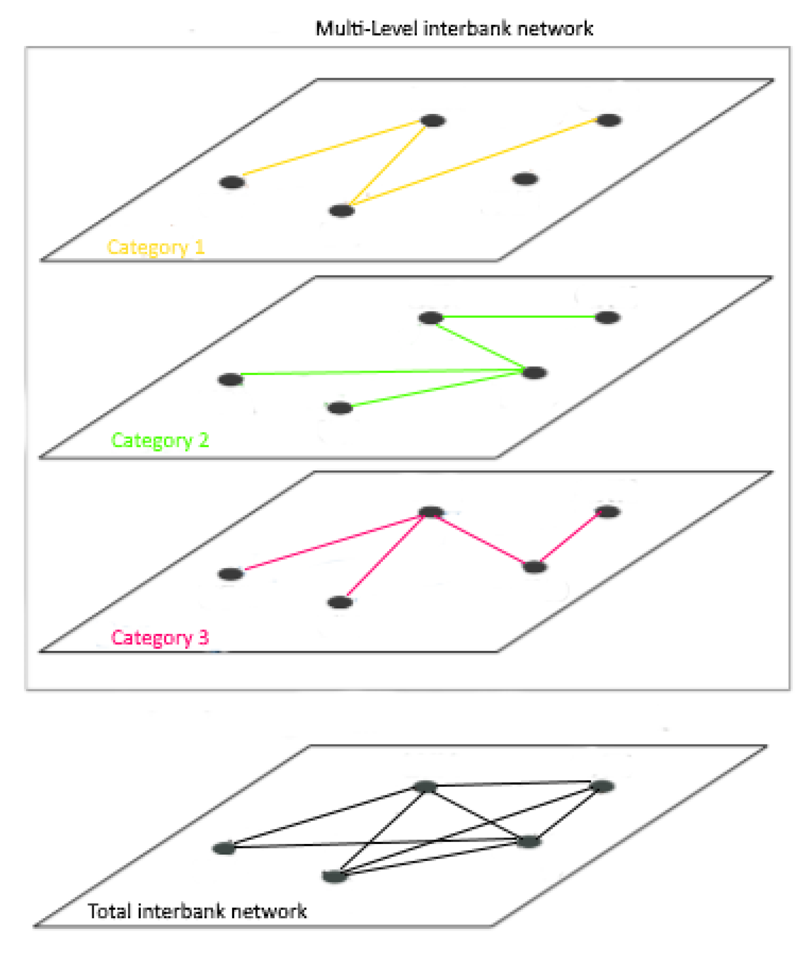
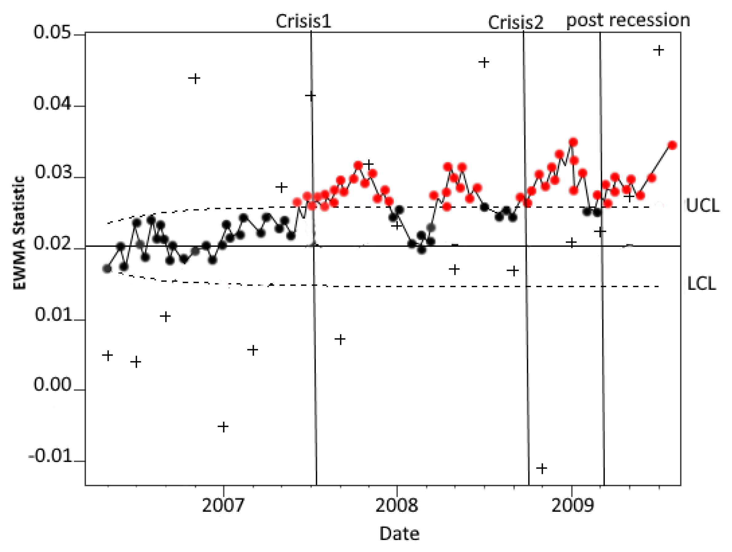
4. Case Study: Change Detection in the Interbank Market during the Financial Crisis

According to reports, the US financial crisis of 2007–2009 slowed economic growth and resulted in high social costs. Furthermore, during the stock market turmoil, the s & p500 index lost half of its value. Thhis crisis highlighted the need to monitor markets and financial institutions [11]. Therefore, the researchers analyzed financial networks and monitored financial markets to illustrate the interrelationships. Financial institutions are considered network nodes in a financial network, and the connections between them are considered network edges. Monitoring financial networks monitors the amount of communication between network nodes. A sparsely connected interbank lending network, for example, could mean that banks have stopped interbank market transactions due to the understanding of systematic risk. We used e-MID data from January 2006 to December 2012 to review and compare the proposed model with the model presented by Ebrahimi et al. (2021) [11]. Each transaction comprises the date, the lender, the borrower, the nation of origin of the lender and borrower, the interest rate, the quantity, the number of trades, and a statement of which party initiated the transaction (with their true names anonymized). A total of 50–60 publicly traded banks are represented in the statistics. The precise quantity is withheld to maintain anonymity because interbank market bank identities are obscure. From the stock market, we obtain the weekly returns of the banks. This article’s type of financial network is the direct relationship between financial institutions, including credit relations. Because there are different links between two institutions, each of which belongs to a class, the interrelationships between two financial institutions are highly complicated. Analyzing these links in different classes is suitable for systematic risk analyses. Therefore, it is better to model this situation with a multiplex network, consisting of several layers, each of which has the same nodes, and only the edges and the weight of the edges are different. A multiplex network with various connections between its nodes can be represented as a network since the network nodes in each layer are the same. Figure 2 illustrates an example of a multilevel network.

The probability of an edge between two nodes of the network in the general network is equal to the probability of an edge between two nodes of the network in at least one of the layers:

$$\mathrm{p}({\mathrm{w}}_{\mathrm{k}\mathrm{d},\mathrm{t}}>0)\sim \mathrm{p}({\mathrm{w}}_{\mathrm{k}\mathrm{d},1,\mathrm{t}}>0)\vee \mathrm{p}({\mathrm{w}}_{\mathrm{k}\mathrm{d},2,\mathrm{t}}>0)\vee \dots \vee \mathrm{p}({\mathrm{w}}_{\mathrm{k}\mathrm{d},\mathrm{J},\mathrm{t}}>0)$$

“In 2012, about 78 percent of the Italian interbank market’s volume was transacted between two banks from the same group, while just 22 percent was intergroup lending” [28]. Since systematic risk is spread through intergroup lending, we consider the network of banking groups in six categories based on the loan exchanges presented in Bargigli, di Iasio, Infante, Lillo, and Pierobon (2016) [28]:

• Overnight (OVN) transactions. Unsecured (U) loans, i.e., without collateral. (OVNU).
• Overnight (OVN) transactions. Secured (S) loans, i.e., with collateral. (OVNS).
• Short-term (ST) transactions, namely those with maturity up to 12 months, excluding overnight. Unsecured (U) loans, i.e., without collateral. (STU).
• Short-term (ST) transaction, namely those with maturity up to 12 months, excluding overnight. Secured (S) loans, i.e., with collateral. (STS).
• Long-term (LT) transactions, namely those with the maturity of more than 12 months of consideration. We distinguish collateralization. Unsecured (U) loans, i.e., without collateral. (LTU).
• Long-term (LT) transactions, namely those with the maturity of more than 12 months of consideration.

Banks do not pay high-risk loans with unsecured collateral when they feel threatened. Therefore, the probability of edge formation between network nodes in various groups differs. In this case, a network analysis using single-layer network methods does not provide accurate results. As stated in [20], there was a 73.68% dispersion rate among all possible banking transactions in the pre-crisis period. We consider banks as network nodes to monitor the financial exchange network between banks in the e-MID market network. Meanwhile, the characteristics of nodes, edges, and network layers are defined as independent variables in the proposed model as follows [11]:

We utilize the lender and borrower returns as node attributes. The lender’s return is the average stock market return of the lending bank in week $\mathrm{t}-1$, and the borrower’s return is the average stock market return of the borrowing bank in week $\mathrm{t}-1$. The return correlation, number of trades, and rate (the average interest rate of each loan between two banks in week $\mathrm{t}-1$ (if any transaction occurred)) are used as edge attributes. The return correlation measures the correlation between the returns of the two banks from the beginning of the data up to week $\mathrm{t}-1$.

It is important to note that we utilized nation (an indicator variable that is one if two banks are different) and ratio (the ratio of layer financial transaction volume to total financial transactions) as random effects and layer attributes (${\mathrm{G}}_{\mathrm{j},\mathrm{t}}={\mathrm{H}}_{\mathrm{j},\mathrm{t}}$). Finger et al. discuss the country difference (2013); community banks lend primarily to the areas where their depositors live and work as opposed to banks that may accept deposits in one state while making loans in another. This helps to maintain and grow local communities.

The majority of the other factors are primarily based on stock market results. Stock market performances can affect a bank’s interbank trading activity, particularly if they significantly impact the bank’s balance sheet (Brunetti et al., 2019 [29]). We, therefore, expect the need for return-based variables, particularly during periods of high stock market volatility, such as during crisis sub-periods. Because these data are generated immediately following a transaction, we did not incorporate the number of transactions and rates in the logistic regression model.

To monitor the real data network, we used data from 20 weeks before the crisis as controlled observations, based on which the initial values of F and Q were calculated. Based on Pearson’s residual errors from the in-control data, we determined the control limits for the in-control ARL to equal 200 ($\mathsf{\alpha }\sim 0.005)$. According to the proposed method by Nishina (1992) [30], to estimate the EWMA change point after receiving an out-of-control signal at time T, the proposed method detected the first changes on 10 April 2007 (where the out-of-control signal is above the upper control limit (UCL) in Figure 3), which was the diagnosis before August 2007, when banks worldwide revealed acute liquidity shortages [29]. The European Central Bank raised interest rates on 6 June 2007 (European Central Bank, 2007). Rational expectations from this action have put loan exchanges under control until the threshold of 2008. The crisis continued until early 2009 after the Wall Street bailout was approved, ending the tremendous financial crisis by keeping the banks active. Findings show that the model identified pre-crisis points with higher accuracy than the online Hurdle model [11]. Figure 3 shows the Pearson residual monitoring results for crisis diagnoses.

5. Conclusions

In this study, we developed a model to monitor sparsely attributed multilevel network streams with dynamic structures. To do this, we hypothesized that the likelihood that two network nodes would form an edge at time t depends on the characteristics of network edges, network nodes, and categories or groupings. Then, we estimated the model parameters using the expressed logit model. The model parameters were developed using the state-space model to achieve the dynamic state in the system. The extended Kalman filter updated state-space parameters and predicted upcoming networks. The proposed model was compared to the online Hurdle model [11] to evaluate the performance by implementing three scenarios. The results show that the model is faster at detecting the first change. Finally, using real e-MID data, we measured the model’s performance in detecting real data changes. The findings suggest that the proposed model may predict a crisis before it arises and detects changes more precisely and quickly than the online Hurdle model [11]. As a result, the random effects of groups and categories in detecting network changes can be considered using this method, which improves the model’s accuracy. Finally, it is recommended that the proposed model be combined with clustering methods to analyze data in which groups and categories are unknown. Additionally, a mixed model approach must be used to consider both within- and between-subject variabilities when drawing the concluding group’s functional magnetic resonance imaging (fMRI) data. The results only apply to participants in the study and not the sample population if a mixed effects model is not utilized to examine the sparse fMRI data [31]. The proposed model is recommended to evaluate FMRI data because using a fixed effects model may increase the false-positive test findings.

References

1. Mantegna, R.N. Hierarchical structure in financial markets. Eur. Phys. J. B-Condens. Matter Complex Syst. 1999, 11, 193–197. [Google Scholar] [CrossRef] [Green Version]
2. Slack, N.; Brandon-Jones, A. Operations and Process Management: Principles and Practice for Strategic Impact; Pearson: London, UK, 2018. [Google Scholar]
3. Trier, M. Research note—Towards dynamic visualization for understanding evolution of digital communication networks. Inf. Syst. Res. 2008, 19, 335–350. [Google Scholar] [CrossRef] [Green Version]
4. Grandjean, M. A social network analysis of Twitter: Mapping the digital humanities community. Cogent Arts Humanit. 2016, 3, 1171458. [Google Scholar] [CrossRef]
5. Hagen, L.; Keller, T.; Neely, S.; DePaula, N.; Robert-Cooperman, C. Crisis Communications in the Age of Social Media: A Network Analysis of ZikaRelated Tweets. Soc. Sci. Comput. Rev. 2018, 36, 523–541. [Google Scholar] [CrossRef]
6. Brennecke, J.; Rank, O. The firm’s knowledge network and the transfer of advice among corporate inventors—A multilevel network study. Res. Policy 2017, 46, 768–783. [Google Scholar] [CrossRef]
7. Harris, J.K.; Luke, D.A.; Zuckerman, R.B.; Shelton, S.C. Forty Years of Secondhand Smoke Research. Am. J. Prev. Med. 2009, 36, 538–548. [Google Scholar] [CrossRef] [PubMed]
8. Finger, K.; Fricke, D.; Lux, T. Network analysis of the e-mid overnight money market: The informational value of different aggregation levels for intrinsic dynamic processes. Comput. Manag. Sci. 2013, 10, 187–211. [Google Scholar] [CrossRef] [Green Version]
9. Azarnoush, B.; Paynabar, K.; Bekki, J.; Runger, G. Monitoring Temporal homogeneity in attributed network streams. J. Qual. Technol. 2016, 48, 28–43. [Google Scholar] [CrossRef]
10. Gahrooei, M.R.; Paynabar, K. Change detection in a dynamic stream of attributed networks. J. Qual. Technol. 2018, 50, 418–430. [Google Scholar] [CrossRef] [Green Version]
11. Ebrahimi, S.; Reisi-Gahrooei, M.; Paynabar, K.; Mankad, S. Monitoring sparse and attributed networks with online Hurdle models. IISE Trans. 2021, 54, 91–104. [Google Scholar] [CrossRef]
12. Mucha, P.J.; Richardson, T.; Macon, K.; Porter, M.A.; Onnela, J.P. Community structure in time-dependent, multiscale, and multiplex networks. Science 2010, 328, 876–878. [Google Scholar] [CrossRef] [PubMed]
13. Lee, K.M.; Kim, J.Y.; Cho, W.K.; Goh, K.I.; Kim, I.M. Correlated multiplexity and connectivity of multiplex random networks. New J. Phys. 2012, 14, 033027. [Google Scholar] [CrossRef]
14. Min, B.; Goh, K.I. Multiple resource demands and viability in multiplex networks. Phys. Rev. E 2014, 89, 040802. [Google Scholar] [CrossRef] [PubMed] [Green Version]
15. Carley, K. A theory of group stability. Am. Soc. Rev. 1991, 56, 331–354. [Google Scholar] [CrossRef] [Green Version]
16. Hollway, J.; Koskinen, J. The case of the global fisheries governance complex. Soc. Netw. 2016, 44, 281–294. [Google Scholar] [CrossRef]
17. Bargigli, L.; di Iasio, G.; Infante, L.; Lillo, F.; Pierobon, F. The multiplex structure20 of interbank networks. Quant. Financ. 2015, 15, 673–691. [Google Scholar] [CrossRef] [Green Version]
18. Almasi, A.; Eshraghian, M.R.; Moghimbeigi, A.; Rahimi, A.; Mohammad, K.; Fallahigilan, S. Multilevel zero-inflated Generalized Poisson regression modeling for dispersed correlated count data. Stat. Methodol. 2016, 30, 1–14. [Google Scholar] [CrossRef]
19. Courgeau, D.; Franck, R. Methodology and Epistemology of Multilevel Analysis: Approaches from Different Social Sciences; Springer: Berlin/Heidelberg, Germany, 2003. [Google Scholar]
20. Fávero, L.P.; Hair, J.F.; Souza, R.F.; Albergaria, M.; Brugni, T.V. Zero-inflated generalized linear mixed models: A better way to understand data relationships. Mathematics 2021, 9, 1100. [Google Scholar] [CrossRef]
21. Fávero, L.P.L. The zero-inflated negative binomial multilevel model: Demonstrated by a Brazilian dataset. Int. J. Math. Oper. Res. 2017, 11, 90–106. [Google Scholar] [CrossRef]
22. Lambert, D. Zero-inflated Poisson regression, with an application to defects in manufacturing. Technometrics 1992, 34, 1–14. [Google Scholar] [CrossRef]
23. Lee, A.H.; Wang, K.; Scott, J.A.; Yau, K.K.; McLachlan, G.J. Multi-level zero-inflated Poisson regression modelling of correlated count data with excess zeros. Stat. Methods Med Res. 2006, 15, 47–61. [Google Scholar] [CrossRef] [PubMed]
24. Fávero, L.P.L.; Serra, R.G.; dos Santos, M.A.; Brunaldi, E. Cross-Classified multilevel determinants of firm’s sales growth in Latin America. Int. J. Emerg. Mark. 2018, 13, 902–924. [Google Scholar] [CrossRef]
25. Wang, K.; Yau, K.K.; Lee, A.H. A zero-inflated poisson mixed model to analyze diagnosis related groups with majority of same-day hospital stays. Comput. Methods Programs Biomed. 2002, 68, 195–203. [Google Scholar] [CrossRef] [PubMed]
26. Younès, M.; Ezzahid, E.H.; Belasri, Y. Operational value-at-risk in case of zero-inflated frequency. Int. J. Econ. Financ. 2012, 4, 70–77. [Google Scholar] [CrossRef] [Green Version]
27. Brown, R.G.; Hwang, P.Y. Introduction to Random Signals and Applied Kalman Filtering: With MATLAB Exercises and Solutions; Wiley: New York, NY, USA, 1997; Volume 12, pp. 35–45. [Google Scholar]
28. Bargigli, L.; di Iasio, G.; Infante, L.; Lillo, F.; Pierobon, F. Interbank markets and multiplex networks: Centrality measures and statistical null models. In Interconnected Networks; Springer: Berlin/Heidelberg, Germany, 2016; pp. 179–194. [Google Scholar]
29. Brunetti, C.; Harris, J.H.; Mankad, S.; Michailidis, G. Interconnectedness in the interbank market. J. Financ. Econ. 2019, 133, 520–538. [Google Scholar] [CrossRef] [Green Version]
30. Nishina, K. A comparison of control charts from the viewpoint of change-point estimation. Qual. Reliab. Eng. Int. 1992, 8, 537–541. [Google Scholar] [CrossRef]
31. Mumford, J.A.; Poldrack, R.A. Modeling group fMRI data. Soc. Cogn. Affect. Neurosci. 2007, 2, 251–257. [Google Scholar] [CrossRef] [PubMed]
Figure 1. Comparison of average run length (ARL) using simulation data in the performances of different scenarios. Smaller ARL values indicate better performances.
Mathematics 10 04483 g001
Figure 2. Schematic representations of multilevel interbank networks. Each node is a bank, and links represent credit relations. The network in black is the total interbank market, obtained by aggregating all layers.
Mathematics 10 04483 g002
Figure 3. EWMA charts for Pearson’s residuals from the zero-inflated generalized linear mixed model to detect the onset of Crisis 1. Red dots are considered as out of control data.
Mathematics 10 04483 g003
Publisher’s Note: MDPI stays neutral with regard to jurisdictional claims in published maps and institutional affiliations.