Abstract
This paper evaluates the deposit and purchase pricing of purchase contracts in a risk-neutral framework. First, we determine the fair deposit price of a single-installment purchase contract based on theoretical modeling and numerical analysis. Second, the buyer’s threshold pricing in dual-installment and multi-installment contracts is investigated under the framework of compound options. Lastly, the pricing behavior of deposits and purchases is further analyzed using a simultaneous equations modeling framework.
MSC:
39-08; 65C30
1. Introduction
The deposit trade, sometimes also known as pre-sale trade, is a trade practice that already prevails in Japan, South Korea, mainland China, Taiwan, and parts of the United State. Examples of such trades include transactions on residential condominiums, pre-sale purchases of residential housing in Asia, and the sales of condominiums on Alabama’s Gulf Coast where most of the units are sold on a pre-sale basis. In addition, the pre-lets trade in the United Kingdom is similar to pre-sale. It is defined as the leasing transactions that have occurred before construction has started. More than 2.3 million square feet of Central London office were taken up in the first quarter of 2018 and 28 percent was undertaken on a pre-lets basis (data collected from 2018 reports of Jones Lang LaSalle (JLL)). In the United States, part of the reason these deposit trades are made possible is because the rights and obligations related to both sides of the transaction are disclosed in great detail in Section 24 of the “Condominium Property Act” of the State of Illinois and in clause 718.202 of the “Condominium Act” of the State of Florida (for legal information and statements for the relevant Condominiums Act, please see the Illinois Complied Statutes (ILCS) and JD Supra available at the websites https://www.ilga.gov/legislation/ilcs and https://www.jdsupra.com/legalnews/2021-legislature-clarifies-use-of-3417731/, accessed on 4 May 2021). In addition, the pre-sale trade in the real estate market also reflects the market investor’s expectation and the variations of future economic conditions [1,2]. In particular, DiPasquale and Wheaton developed a structural model of the single-family housing market and analyzed how consumers form expectations about future house prices. They found the evidence from gradual price adjustment when consumers develop expectations by historical price movements and based upon rational forward-looking forecasts. Therefore, the deposit trading system has undoubtedly helped the efficiency of the real estate market. In the existing literature, some studies have also been devoted to investigating the relationship between pre-sale activity and cycles in real estate markets [3], to analyze the effects of economic conditions on pre-sale trade [4], and to examine the buyer’s preferences [5]. However, for a long time, few substantial theoretical research studies have been published in this area. Additionally, lacking a fair standard as well as any significant progress to improve the theoretical framework, disputes on the proper valuation of transactions related to deposit payments do occur on many occasions.
In contrast with the assumptions of previous studies, the purpose of this paper aims to determine the fair amount of deposits for various installment contracts, to relax the assumptions of the exogenous nature of purchase price, and to investigate the effects of market condition changes on the pre-sale trade. To do this, using a risk-neutral hypothesis, we attempt to establish a theoretical model to deal with problems of determining the fair deposit and purchase prices in response to the deficiencies described above, as well as to model the determination of fair prices under the conditions of arbitrage-free pricing, which precludes a special “out-clause” (in some areas of the US, the buyer could recover the deposit even though the property was not purchased. For example, clause 718.202 of the “Condominium Act” of the State of Florida shows that (a) if a buyer properly terminates the contract pursuant to its terms, the funds shall be paid to the buyer or, (b) if the buyer defaults in the performance of his or her obligations under the contract of purchases and sale, the funds shall be paid to the developer) as a legitimate way to exit the market under our modeling framework, although we might consider modeling such behavior in forms related to implicit options in future research. It is worth mentioning that in business practices the actual amount of the deposit is often a lump sum payment that is not sensitive to the market condition as well as the specifics of the purchase transaction. Business practices notwithstanding, in this article we assume that the desirable amount of the deposit will be fairly priced by a theoretical model and not be determined arbitrarily by the seller.
In the past, Ref.[6] (hereafter SBS) used contingent claim analysis to study the deposit of newly constructed residential condominiums in the Baton Rouge area in Louisiana. The SBS paper provides a very good analytical framework for evaluating the embedded options in real estate contracts. However, they may overlook the requirement that the contract price must be equal to the amount of the deposit on the contract signing date. Furthermore, their model applies only to single- but not multi-installment deposit contracts. Lastly, they treated the purchase price of residential condominiums as an exogenous variable in their model. Therefore, Ref.[7] used the option pricing model to evaluate the fair deposit of the contract over two periods. The author found that the characteristics of multi-installment contracts play an important role in the valuation of fair deposits. However, the research does not discuss the variation of fair deposits when market conditions change. In addition, Ref.[8] further investigated the effect of depreciated rate and default premium on pre-sale housing prices using an option pricing model and showed that the model provides good forecasting accuracy. Similarly, Ref.[9,10] have applied the option theory to property market analysis. They argued that the variations of options value can effectively reflect the adjustment costs and future volatility. In addition, Ref.[11] also argued that traditional and standard discounted cash flow valuation techniques are unable to deal with a variety of options contained in lease contracts. Thus, if the buyer ignored the options value of purchase price and deposit in pre-sale trade, they may make a wrong decision.
On the other hand, Ref.[12] found that fundamental insights of real options theory are evident to individual investors using the experimental methodology. They argued that the majority invested too early and thus failed to recognize the benefit of the option to wait. Consequently, to further know the valuation of contract deposit and purchase price and to consider the deposit trade holding the characteristics of options contracts, this study uses the risk-neutral hypothesis to set up an integrated theoretical model to determine the fair amount of deposits for single- and multi-installment contracts. The same modeling approach can also be extended to the determination of the purchase price and the amount of deposits in a simultaneous equations setting as will be discussed later in this article.
Firstly, we describe how the practice of deposit payments would help formulate the contracting process in a real estate deal. Generally speaking, after negotiating the purchase price and the amount of deposit with the seller, the buyer usually settles his/her transaction with a “hard contract”, which is a binding sales contract that outlines the details of the entire project and the amount the buyer needs to pay in order to purchase the agreed-upon unit. After signing a hard contract, the buyer is usually required to pay a deposit either on a single- or multi-installment basis to the seller in exchange for the right (but not obligation) to purchase the underlying asset within a specific period. The length of the time period before the buyer can exercise the hard contract could vary between several days and a few years.
In the rest of the modeling process, this study assumes that the deposit will be confiscated by the seller if the buyer does not honor his/her obligations on additional deposit payment dates (if any), or the buyer will exercise the contract on the closing date according to the purchasing contract. For convenience, the “fair” amount of deposit refers to the amount that is acceptable to both the buyer and the seller when all specifications in the contract in question have been satisfied. In other words, it is the amount that “clears the market” under the given terms and conditions that are acceptable to both sides of the transaction.
Under this trading practice, the buyer has plenty of time to reconsider his/her original purchasing decision after the initial deposit payment is made. The seller also receives indemnification for the risk he/she takes in case the buyer breaks his/her initial purchasing promise. Although officially the amount of the deposit that the buyer needs to pay is usually only 10 percent of the agreed-upon purchasing price, in practice the seller often asks for deposits that double the official percentage. It is also observed in the marketplace that the buyer often reserves the right to resell his/her contract to a third party when such transactions are allowable. We can now consider the generalized process of deposit trades when the seller requires the buyer to make multiple deposits at different stages of the construction process. For example, in pre-sale housing some sellers in mainland China and Taiwan require buyers to make multiple deposits that correspond to their multi-installment construction plan. Therefore, one of the focal points of this paper is to determine the fair multi-installment deposits when the construction is multi-staged.
This study determines a “threshold price” for each stage of the construction process when the buyer is required to pay for deposits on a multi-installment basis. In pre-sale housing, this means that the buyer has the choice of deciding if he/she would pay for additional deposits at the due times by comparing the prevailing market price of the underlying housing unit with a critical price he/she has in mind. If the current housing price is higher than his/her critical price, then the buyer keeps paying for the deposits; otherwise, he/she chooses to break the contract by not paying them. We call this critical price the threshold price, and we will derive its theoretical value by using the option-theoretical approach later in this paper.
The multiple-deposit paying process described above can be extended to cover the case of condominium pre-selling where the purchase price and the amount of deposit are determined simultaneously. Consequently, after extending the model in order to include this new consideration, we find that the deposit-to-purchase price ratio calculated using our theoretical model (5% to 10%) is very close to the official deposit-to-purchase ratio (10%), but is somewhat lower than the deposit-to-purchase ratio (10% to 20%) that prevailed in the marketplace as was reported earlier. These results authenticate the credibility of our theoretical deposit model that was used to calculate the proper deposit-to-purchase price ratio for the pre-sales of condominiums.
As mentioned above, this study contributes to the theoretical literature on the pre-sale trade of residential condominiums in several areas. First, we determine the fair deposit price of different installment contracts based on the option modeling and compound option modeling. In contrast with SBS, this study analyzes the effects of changes in relevant variables on fair deposit in single-, dual-, and multi-installment contracts, and further investigates whether the time interval between the initial deposit payment and subsequent interim deposits affects the total amount of the deposit. Secondly, applying the risk-neutral valuation approach, the buyer’s threshold pricing is also investigated in different installment contracts. We study how the payment frequencies and the waiting time between installments affect threshold price. Finally, from the viewpoint of market efficiency and non-arbitrary argument, the simultaneous equations setting provides evidence that deposit-to-purchase ratio is very close to the official ratio. It is different from actual deposit ratios charged by sellers in the marketplace. A more detailed analysis will be given below.
The remainder of this paper is organized as follows. Section 2 describes the characteristics of deposit trading systems, part of which will be explained via the viewpoint of modern financial options. Our main theory will be established in Section 3, where each of the topics will be discussed in the following order: (1) the basic assumptions of the overall model, (2) single-installment deposit model, (3) dual-installment deposit model, and (4) modeling for the case of multi-installment deposits. Numerical examples are also provided in Section 3 in order to validate the theoretical results discussed above. Section 4 provides a simultaneous equations model that determines the amount of the deposit and the purchase price concurrently as described earlier. Lastly, Section 5 concludes this paper and suggests some directions for further research.
2. Characteristics of Deposit Trade
The characteristics of deposit trade can be summarized briefly as follows. (1) All deposits that the buyer pays before the final delivery date must be treated as part of the purchasing price for the underlying housing unit. This implies that the final settlement price the buyer pays to the seller on the closing date must be equal to the agreed-upon purchase price minus the total amount of deposits the buyer has already paid for. (2) According to the contract, the buyer does not need to pay any fees other than the deposit(s) in order to secure his/her purchasing activity before final delivery. (3) In case the buyer does not exercise the contract, the seller has the right to confiscate the deposit at closing time.
The main difference between a financial option and deposit trade is that the premium of a financial option is not deductible from the underlying asset’s exercise price, while the paid deposit of a contract is deductible from the purchase price when the buyer exercises the contract. Nevertheless, similarities between a deposit trade and contingent claims do abound, which allow us to construct theoretical models to determine the fair deposits under the single- and the multi-installment agreements using concepts similar to [13] option modeling or [14] compound option modeling.
As discussed earlier, after presenting a fair deposit model under the single-installment environment, the discussion will be extended to cases where the installments can be dual or multiple. We will examine the determination of the deposit and the purchase price in a simultaneous equations setting in the last part of this section. To begin with, Figure 1 describes activities that may occur on each step of the decision tree in the deposit trading process. Cases for the single-, dual-, and multi-installment deposit trading are shown in Figure 1a–c, respectively. Taking multi-installment deposits as an example, a buyer pays an initial deposit () and is liable to pay an additional deposit () on each of the pre-determined dates corresponding to the seller’s cash flow schedule that varies in accordance with the seller’s construction costs. If the buyer does not come up with the required deposit payment when it is due, the seller would have the right to terminate the contract and confiscate the buyer’s deposits. Note that the total deposits already paid for can be deducted from the purchase price () when the buyer makes the final purchasing payment on the delivery date as shown in Figure 1c. Therefore, on each branch of the decision tree the buyer’s adjusted exercise price for the underlying housing unit equals , where .
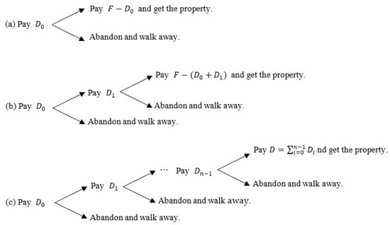
Figure 1.
Decision tree for deposit trading. The is purchase price on the delivery date and denotes the deposit at time .
3. Model Setup and Solution
In this section, we first describe the basic assumptions and then apply the risk-neutral valuation approach to estimate the theoretical amounts of fair deposits under different modeling scenarios.
3.1. Assumptions
Our theoretical model is established based on the assumptions stated as follows.
- (1)
- According to the assumption of the stochastic process followed by geometric Brownian motion, the property value on the decision tree corresponding to each decision date is assumed as log-normally distributed. This implies that the logarithm of the property value () (the property value may change as market conditions change or as the buyer investigates the property. For example, the buyer could choose not to pay an inspection fee, or pay a small fee for a quick inspection, or pay a large fee for a detailed inspection. The different inspection alternatives are likely to lead to different property valuations by the buyer and hence different levels of asset volatility and service flow. However, we only focus on the effect of a market condition change on the property value. Moreover, in this paper we use the log-normal distribution to describe the characteristics of the property value) has an expected drift that equals , where is the risk-free rate that is assumed to be constant during the contract period and is the service (or rental) flow generated from the underlying property. In addition, the variance of S equals , where is the instantaneous volatility of the property price, and is the time period between the contract signing date, , and the maturity date of the contract, . Following [15,16], this study also assumes that the service flow is proportional to the value of the underlying property, S.
- (2)
- Key variables included in the purchase contract and their features are described as follows: (i) it assumes the property purchasing price, , is a fixed number once the model is solved. This assumption will be relaxed later in the next section. (ii) On the other hand, the deposit payment is an endogenous variable. Its estimated value also remains constant until the maturity time of the contract, once the model is solved. (iii) The buyer’s deposit will be confiscated if he/she violates the terms and conditions of the contract.
- (3)
- We assume further that the contract can be traded without transaction costs. It follows that the market price of the contract, , is a function of the following four variables: (1) the property’s market price S, (2) the contract’s term-to-maturity t; (3) purchase price ; and (4) the amount of the deposit .
3.2. Single-Installment Deposit Model
Following SBS, the contract will be worthless on the closing date if the asset price, , is below the settlement price X, where , because the buyer could purchase the asset at a price lower than the settlement price. On the other hand, the contract would be worth if the property’s closing price is above the settlement price. Therefore, on the closing date the contract’s value must satisfy the following boundary condition:
Applying the risk-neutral valuation methodology to Equation (1), the contract’s value at time t can be stated as if it is a call option with strike price :
where represents the cumulative standard normal distribution function. Following Black–Scholes, we define and in as:
Note that Equation (2) is almost exactly the same as Equation (1) in SBS. The only difference is that SBS allows a non-zero closing cost while we allow a non-zero service flow instead.
Under the no-arbitrage condition, the amount of the payment made by the buyer, , must converge to the value of the contract, , at the instant when the contract is signed, i.e., when . Therefore, using Equation (2), the following initial condition must hold if the deposit is “fair” at time τ:
where . The equation above does not have a feasible closed-form solution. Its solution can be found by using numerical methods only if the approximation process converges (the Newton–Raphson method we use is an iterative process to approximate the root solution of a function. Please refer to Chapter 2 of [17] for more details about this method). In the rest of this section, we will discuss the behavior of fair deposits using the concept of comparative statics before we present a stable solution for Equation (3).
We first derive the following results needed for a comparative static analysis for the behavior of fair deposits by total differentiating Equation (1). Signs associated with each differentiation represent the directions of changes of with respect to other variables under consideration.
where represents the probability density function of the standard normal distribution.
According to Equation (4), the amount of the deposit, , will be higher when purchase price becomes lower. This is because the buyer would pay a higher deposit to lock in the seller’s offer price if the purchase price charged by the seller is below the market. Similarly, in Equation (5), if the current housing price becomes higher, then the deposit the buyer is willing to pay should also become higher. The situation for the volatility of the asset price, , is a bit more complicated. Equation (6) implies that the higher is, the higher the deposit becomes. This result is related to the fact that the deposit contract is in fact an option on the underlying housing unit. The buyer has great upside benefits when the asset’s price is rising, but few downside risks when the asset’s price is falling. As a result, the buyer’s upside benefits must increase together with the asset’s volatility.
According to Equation (7), the asset’s service flow, , and its deposit move in opposite directions. This is because higher service flow increases the buyer’s cost of owning the contract, which could depress his/her willingness to pay for a high deposit that can be considered as an opportunity cost for the buyer when he/she makes home-buying decisions. An alternative explanation is that a higher periodic service payment increases the cost of house ownership, which contributes negatively to the cash flow discounting process when we evaluate the realized value of the contract.
Equation (8) shows that the risk-free interest rate has a positive effect on the amount of the deposit. Specifically, the risk-free rate has two effects on deposits. First of all, the risk-free rate is used to discount the terminal (risk-neutral) cash flow to determine a contract’s value and its fair deposit. Thus, a higher risk-free rate will lead to a lower contract value as well as a lower deposit. Second, a higher risk-free rate means the contract holder is more likely to realize a higher cash flow at maturity date if the asset’s value grows at a faster rate in the risk-neutral world. While these two effects push the values of the deposit in opposite directions, the second effect should dominate the first at the end. In summary, the deposit’s value should increase as the risk-free rate increases.
Depending on whether the net effect due to changes in terms in the bracket of Equation (9) is positive or negative, the influence of the contract’s maturity date, , on the amount of the deposit is ambiguous at best. The effects are explained as follows. The first term in the bracket shows that is positively related to the deposit, because an increase in increases the probability that the price of the asset will go up, which creates a positive effect on the value of the deposit payment. On the other hand, the second term indicates that the service flow from holding the asset increases when increases. As we have learned already from the discussion earlier, an increase in service flow decreases the deposit, so that should be negatively related to the amount of the deposit. Lastly, the third term reveals that the present value of the settlement price decreases when T increases. Consequently, lengthening T creates a positive effect on the amount of the deposit.
3.3. Dual-Installment Deposit Model
In the dual-installment deposit model, we assume that the buyer has to pay a second deposit, , on the interim payment date in addition to the first deposit, . The model is created in response to the fact that some of the contracts in pre-sale housing require additional deposits to cover both the initial construction cost and the subsequent multi-installment construction costs separately. If the buyer does not pay the second deposit according to plan, then the seller has the right to terminate the contract and confiscate the buyer’s initial deposit. This dual-installment model will be extended to multi-installments in the next section in order to provide a general theoretical framework to cover this type of contract in the marketplace.
Since the buyer stands to lose the right to buy the underlying asset if he/she misses the second deposit payment, an alternative explanation toward the buyer’s motive of paying for the first deposit, , is securing the right to purchase the second-period contract with a fixed value, , on the date of interim payment. Therefore, this study split the buyer’s decision into two separate steps. First, we can treat as a call option on , which is a call option by itself on the underlying asset before the final purchase. Therefore, the whole concept is similar to buying a “call-on-call” or “split-fee option” as described in [14] compound option model. Following the same argument we made for establishing Equation (1), this compound option contract must satisfy the following boundary condition at maturity:
As stated in [14], we can solve Equation (10) by utilizing the risk-neutral valuation methodology. Therefore, the closed-form solution for the second-period contract, , can be stated as follows.
If the buyer chooses to exercise the contract on the day of interim payment, , then he/she will face the following two potential decisions. First, if the value of the second-period contract () is lower than , then the contract will not be exercised and its value is zero. Next, if the value of the second-period contract is higher than , then the contract will be exercised and the value of the first-period contract will be equal to that of the second-period contract minus . The discussion above can be summarized by the following equation:
Using Equation (12), we can derive the theoretical value of the first-period contract, , whose time domain covers the period between the initiation date of the contract and the day when the interim payment is made:
In the above equation is a bivariate cumulative standard normal distribution function and is asset price at time , such that . In other words, is the critical price for the buyer to determine if he/she is willing to pay for the second deposit () on the date of interim payment. He/she chooses to pay for if the price of the underlying asset is higher than and forfeits the contract if the price of the underlying asset is lower than . Following the set of initial conditions similar to those stated in the single-installment deposit model, we derived the following equation to evaluate both and in the dual-installment model.
where is from Equation (13). Note that Equation (14) consists of two variables ( and ) and is under-identified if we seek the solutions for both. Therefore, it needs to include an additional condition to make the equation solvable. One of the ways is to hypothesize that the amount of the initial deposit the seller requests equals that of the interim deposit, . Another hypothesis is . In practice, the relative values among and for i = 1, 2, … n are usually maintained at an agreed-upon level when the first deposit payment is made. Solutions for Equation (14) under and are presented in Table 1.

Table 1.
Fair Deposits for Single-Installment and Dual-Installment Models.
In summary, Equations (3) and (14) as well as pre-determined relationships between and are used to solve for the single- and dual-installment deposit models using the Newton–Raphson method (the numerical algorithm for computing the fair deposit is programmed in Mathlab 6.0 software, whereby the tolerance error level is less than 0.0001). Table 1 presents solutions for single- and dual-installment deposits under different combinations of closing dates () and interim payment dates (). Two different hypotheses on the payment schedule, namely and , are used to address the issue of how sellers could request single and dual deposits. For example, when 1 and 0.5, the optimal solution for the single-deposit model is 15.52. On the other hand, solutions for the dual-deposit model when are 12.18 and 6.09. Implications of results shown in Table 1 are presented in detail as follows:
- (1)
- On the date of interim payment, the buyer exercises the contract and pays the interim deposit () if the market price of the underlying asset is higher than the threshold price (= 86.96). Otherwise, the buyer chooses not to pay and the contract will be forfeited. Note that the total value of deposit payments, , under the dual-deposit model (18.27) is greater than that under the single-deposit model (15.52), because the former arrangement gives the purchaser greater flexibility in his/her decision-making process. Similarly, for the dual-deposit model under the hypothesis when , the total deposit value (20.98) is greater than that under the alternative hypothesis when (18.27), because the purchaser needs to pay a greater up-front deposit when .
- (2)
- Another interesting observation is that the total deposit values of the dual-deposit payment model converge to the deposit amount solved for the single-deposit model when t1 diminishes. For example, when t1 equals 0.1, the total deposit value under the alternative model converges to 15.93, which is quite close to the solution for the single-deposit model (15.52). In fact, when becomes smaller and approaches , the total amount of dual-installment deposits under either hypothesis converges to a constant that equals the optimal deposit value solved for a single-deposit model.
- (3)
- Assume either that the closing date () or the length of the time period between the date of interim payment and the closing date () is fixed. The values of the initial deposit, the interim deposit, and their total amount will all become smaller if we move the payment dates closer to the date when the contract is originally initiated.
Note in the discussions above that the buyer’s threshold price does not change monotonically as the date of interim payment varies. This result is different from Geske’s compound call option model, because in the latter case both the interim and final exercise prices are treated as exogenous variables. On the other hand, in our model both the interim payment (, relative to the interim exercise price of the compound call option model) and the settlement price (, relative to the final exercise price of the compound call option model) are treated as endogenous variables. Therefore, while in the compound call option model an increase in either or the interim (or the final) exercise price will increase the critical price, in our model an increase in will cause to increase, but to decrease. Given that increases in either or will lift the values of and decreases in will depress the values of , whether will increase or decrease when increases will depend on the net results created from the above two effects. Directions of the net effect notwithstanding, changes in S* are a non-linear function with respect to changes in .
3.4. Multi-Installment Deposit Model
In this section, we will extend the single- and dual-deposit models discussed in the last section into a multi-installment model. In addition to paying for the first deposit when , we assume the buyer has to pay deposit up to the ()th period of the contract when the deposit payment equals . For convenience of discussion, in the rest of the paper we will use to represent the ith payment date when . We assume again that the seller has the right to terminate the contract and confiscate all of the buyer’s previous deposits if the buyer does not renew the contract by paying up the additional deposit according to plan on any of the requested deposit payment dates.
Following the same framework as that discussed earlier, we define the ith contract as an individual contract covering time interval (), within which buyers that hold the ith contract have the right to purchase the i + 1th contract by paying in the ith payment period. Finally, when i = n, buyers have the right to purchase the underlying asset by paying at the closing date . For convenience of discussion, we now define a set of simplified assumptions and notations as that stated in the following equations.
Note that in Equation (15) represents the value of the i + 1th contract that includes the initial contract date when i = 0. In addition, in Equation (16) represents the closing date, in Equation (17) represents the underlying price at , and in Equation (16) represents the settlement price of the deposit. Equations (17) and (18) show that holders of the nth contract after paying have the right to purchase the underlying asset that is worth at closing date . In general, when the buyer holds the ith contract (), he/she has the right to purchase either a new contract by paying or to purchase the underlying asset that is worth . If the buyer chooses to exercise the contract instead, then purchasing the i + 1th contract for is equivalent to purchasing the underlying asset for . As a result, the ith contract can be evaluated as:
On the initial contract signing date (), the buyer could purchase the contract at price . Therefore, the initial condition can be stated as follows:
Consequently, we obtain the following results from Equation (19):
where and
- and
- where .
Equation (22) is recursive solving that requires knowledge about . Solutions for can be obtained by using the backward induction method since we already know . However, in order to obtain solutions for all the Cis simultaneously, we still need the help of using the seller’s deposit collection rules, because the equation is under-identified. We could hypothesize , where equal amounts of deposits will be collected by the seller in every installment. Nevertheless, solving the recursive integral equation as shown above is a complicated process and the assumption that the distribution is multi-normal is not sufficient to simplify the valuation process if the number of interim payments is greater than two periods. Therefore, we will use the following numerical examples to help us explain the characteristics of multi-installment deposits and their threshold prices at different payment dates.
Table 2 shows the numerical results of a multi-installment model after solving Equation (22) using the finite difference method. In this table, we individually simulate the deposits and threshold prices for contracts with 3, 4, 6, and 12 installments. Taking the contract with four installment deposits as an example, we assume the contract’s sign-on date is 1 January and the closing date is 31 December. Assume further that both the contract’s price () and spot price () equal USD 100 and the deposit payments occur on 1 January, 1 April, 1 July, and 1 October. If we assume the amount of the required deposit at each installment is the same, then the optimal deposit that would be paid on each interim deposit payment date is USD 6.54 and the threshold prices on April, July, and October should equal USD 93.30, USD 86.70, and USD 80.20, respectively.
Table 2.
Fair Deposits under Single-, Dual-, and Multi-Installment Payments.
The buyer’s decision rules can now be summarized as follows. Assume he/she has already paid USD 6.54 on the initiation date of the contract (1 January). He/she should pay for the second installment deposit if the observed underlying price is higher than USD 93.30 on the second payment date (1 April), and forfeit the contract otherwise. Decision rules for other payment dates can be deduced similarly. Lastly, the threshold price on the closing date (31 December) equals the contract’s settlement price at USD 73.84 (=100 − 26.16).
In conclusion, Table 2 shows that an increase in the number of deposit payment installments has the effect of suppressing the amount of deposits paid in each installment, but increasing the total amount of the deposits collected by the seller. Moreover, as the time value of the contract diminishes to zero, the optimal threshold prices correspond to the interim payments on different deposit payment days, converging to the settlement price, which equals the original purchase price less the accumulated deposits and should be lower than any of the threshold prices. The consideration prompts the threshold price to fall as time elapses.
4. The Compete Model
In this section, we will extend the model by relaxing the assumption that the purchasing price is treated as an exogenous variable. The new assumption allows us to determine the purchase price and the contract’s deposit amount simultaneously. Assume the buyer has funding whose amount equals the current value of the property, . Assume further that the buyer has the choice of using the funding either to buy a purchasing contract (before he/she decides to buy the real estate) or the underlying property directly. The rate of return under the two strategies can be calculated separately as follows:
- Strategy A: Buy and hold the underlying property until the closing date and at the same time realize the service flow. The rate of return of strategy , , is:
The first term on the right-hand side of the above equation is the capital gain of holding the underlying asset. The second term is return from service flow. By using the risk-neutral valuation methodology, the expected return from strategy A can be written as:
where denotes the expected value in a risk-neutral world.
- Strategy B: Sign a purchase contract and pay a deposit. The rate of return, , on the closing date would be:
Equation (25) consists of two parts. The first part shows that when the market price is higher than the final payment on the closing date, i.e., when , the buyer chooses to exercise the contract. The payoff as shown in the numerator part of the equation equals: (i) the difference between the property value at time and the purchasing price at time , , plus (ii) principal and interest of the initial funding excluding deposit, , and minus (iii) the initial funding, .
The second part of Equation (25) shows that if the market price of the asset is lower than the final payment, i.e., if , then the buyer discards the contract rather than exercising it. Consequently, the deposit will be confiscated and the buyer’s net gain is only . Applying the risk-neutral valuation methodology to Equation (23), its solution can be derived as follows:
Under the non-arbitrary argument, the expected returns from the two strategies should be equal. By comparing Equations (24) and (26), we obtain the following equation:
Equation (27) illustrates an implicit relationship between the agreed-upon purchase price, , and the deposit level, . It shows that the desirable level of deposit and the purchasing price interact to find an equilibrium point in the marketplace. Therefore, both variables can be treated as endogenous in the model where the optimal values can be solved at time . Specifically, in the single-installment environment, Equations (2) and (27) provide a pair of simultaneous equations that could be used for finding the optimal level of deposit, , and the optimal amount of purchase price,, at the same time. Numerical methods such as Newton–Raphson can be used to solve the equations, because both are non-linear.
Detailed discussions on the solutions for the simultaneous equations are presented as follows. First of all, Table 3 shows that increases in purchase price () can be attributed to increases in property price (), the risk-free rate (), closing date (), or decreases in the asset’s service flow (). These results are consistent with our intuitive understanding about the behavior of these variables considering the cost-of-carry when we purchase a real estate property. Moreover, a higher purchasing price could also be attributable to an increase in asset price volatility in the case of condominium deposits, because in this case the deposits are not exercisable.
Table 3.
The Deposit and Purchase Price are Endogenous.
We will next use the numerical results reported in Table 3 together with Equations (4)–(9) to explain the implications of “fair” deposits. To begin with, high property prices will create the following two effects in opposite directions: first, they will cause the deposit to become higher according to Equation (5). According to Table 3, the empirical results from our theoretical model found that the deposit-to-purchase ratio is between 5.08% and 7.92% when the housing price becomes higher/lower by (the base parameter assumed is ). In other words, the ratio may greatly increase during extremely high growth of housing prices. From the viewpoint of rational investment, the buyer may choose to pay the reasonable deposit depending on the current market condition. If the deposit is overpriced, the buyer will tend to proceed to strategy A. Therefore, under the non-arbitrary argument, the market mechanism leads to the fair deposit amount. Simultaneously, based on Equation (4), increases in the purchase price will cause the deposit to become lower since buyers would have less incentive to pay for the deposit of housing units that are considered to be “overpriced”. Although the numerical result indicates that the first effect dominates the second, from a theoretical viewpoint it is still ambiguous whether increases in property prices indeed cause the amount of deposit to increase. Third, changes in risk-free rates and the asset’s service flow do not have clear directional effects on deposits either, because effects created due to these two variables go against each other. However, according to the results of the risk-free rate, we find that the positive effect will dominate the negative effect when the time to the contract’s closing date increases to six months. In other words, the highly risk-free rate is more likely to realize higher cash flow at the maturity date if the asset’s value grows at a faster rate in the risk-neutral world. In addition, this paper also shows that a negative relationship commonly exists between an asset’s service flow and deposit, but not in three months and six months. Fourth, changes in the contract’s closing date, T, also have ambiguous effects on the amount of the deposit according to Equation (9) despite the numerical results shown in Table 3 indicating that it has a positive relationship with the amount of deposits. Lastly, changes in price volatility create positive direction and indirect effects on deposits, i.e., the amount of the deposit is higher if the asset price volatility becomes higher, because buyers can consider the deposit as an option.
In conclusion, notwithstanding the theoretical relationships just discussed, the computational results as shown in Table 3 indicate that changes in the contract’s closing dates and asset price volatilities could impose significant effects on the deposit-to-purchase price ratios. Computations for the deposit-to-purchase price ratios in Table 3 cannot be carried out without additional information. By assuming that the amount of deposit the seller receives from the buyer is proportional to the purchasing price, we calculate deposit-to-purchase price ratios using the same model and the same hypothesized values for the parameters stated in the model. Our calculated deposit-to-purchase price ratios range from 5% to 10%. These results are very close to the official deposit ratio (10%), but are lower than the deposit ratios generally observed in the marketplace, which usually range from 10% to 20%.
5. Conclusions
Following SBS, this article uses risk-neutral valuation methodology to determine the fair deposits for single-, dual-, and multi-installment contracts. Furthermore, option-theoretic models have been created to determine the purchase price and the deposit of contracts in a simultaneous equations setting. Although most of the results presented in this article were derived through theoretical modeling and numerical analysis, their main implications in the business world can be summarized briefly as follows.
First, in the single-installment deposit model, factors that contribute to changes in fair deposit have been clearly identified. They include contract price, the market price of the underlying asset, price volatility of the underlying asset, the asset’s service flow, and the risk-free rate. Relationships between the amount of deposits and changes in each of the variables were also analyzed and clearly identified. The only relationship that is ambiguous is how a buyer changes his/her deposit payments in response to changes in closing dates. Second, using the dual-installment deposit model, we find that a decrease in the time interval between the initial deposit payment and the subsequent interim deposit payments creates a positive incentive for the seller to charge higher initial and interim deposits. On the other hand, had we moved the date of interim payment closer to the contract’s initial signing date, the total amount of the deposits under the dual-installment model would converge to the same theoretical level as that derived for the single-installment deposit model. The results from our models find that the buyer’s threshold price is dependent upon several variables, which include the length of time between the two installment deposit payments and the relative value between the amount of interim deposit payment and the settlement price of the underlying property.
Third, after extending the dual-installment model to the area of multi-installments, this study finds that increases in the number of installments have the effects of depressing the amount of deposit that the buyer would pay for each installment, but raising the total amount of deposits the seller would collect. As the time intervals among installments lengthen, the added uncertainty introduced by the extended waiting time between installments increases the threshold price of the interim deposit payment. The values of the threshold price eventually converge to a constant equal to the final settlement price. Finally, assuming that exchanging information between buyers and sellers is free and efficient, we extend the single installment model so that fair levels of deposit and purchase price can be determined simultaneously within the same modeling framework. We are quite surprised to find out that the deposit-to-purchase price ratio derived from the theoretical model is very close to the official ratio, granted that both of the above two ratios are slightly lower than the actual deposit ratios commonly charged by sellers in the marketplace.
Directions for further research should include, firstly, a detailed estimation of model parameters via empirical research based on the theoretical framework developed in this article. In practice, it is possible to change buyer’s willingness to pay for a high deposit. For example, the youth housing subsidy program helps young people obtain the benefit of house loan agreement interest rates, and the urban planning area is expected to raise the value of residential condominiums and to increase the speed of price movement in the real estate market. These factors will change the purchase price and contract’s deposit. Secondly, transaction costs and means for verifying the values of fair deposits should be studied and reported. As far as the buyer is concerned, the cost from pre-sale trade includes the information cost before transaction, the transaction fee during setting a contract, and the cost of warranties to deliver at the maturity date. Therefore, from the perspective of information asymmetry, the changes in the total amount of the deposit are still ambiguous. The relaxation of this assumption is suggested for future research. Thirdly, considerations should also be given to situations when buyers are requested to pay fees in situations such as when the contract is passed along to a third party or when it is exercised before the final contract payment date. Lastly, it would be interesting to extend the models to study situations when sellers are also allowed to break the contract. Under such circumstances, the seller would have to pay a penalty to compensate the buyer’s “fair deposit”. Generally speaking, the new assumption should create an enhanced effect on the value of the buyer’s deposit, because part of the penalty would be used to pay for the buyer’s losses in case the seller breaks the contract. In other market applications, taking into account the uncertainty and flexibility, the real options models provide good understanding to analyze the values in real property leases and long-term investment planning in decision-making.
Author Contributions
Author Contributions: Conceptualization, C.-M.H. and T.-C.C.; Formal analysis, T.-C.C. and C.-M.H.; Investigation, C.-M.H.; Methodology, T.-C.C. and C.-M.H., Project administration, C.-M.H.; Resources, C.-M.H.; Software, T.-C.C.; Supervision, T.-C.C.; Writing—original draft, T.-C.C.; Writing—review & editing, C.-M.H.. All authors have read and agreed to the published version of the manuscript.
Funding
This research received no external funding.
Conflicts of Interest
The authors declare no conflict of interest.
References
- Case, K.E.; Shiller, R.J. The Behavior of Home Buyers in Boom and Post Boom Markets. N. Engl. Econ. Rev. 1988, 29–46. [Google Scholar]
- DiPasquale, D.; Wheaton, W.C. Housing Market Dynamics and the Future of Housing Prices. J. Urban Econ. 1994, 35, 1–27. [Google Scholar] [CrossRef]
- Ko, W.; Zhou, Y.; Chan, S.H.; Chau, K.W. Over-Confidence and Cycles in Real Estate Markets: Cases in Hong Kong and Asia. Int. Real Estate Rev. 2010, 3, 93–108. [Google Scholar]
- Chiou, Y.S.; Chou, M.L.; Chang, C.O. A Prediction Model for Housing Investment Probability. NTU Manag. Rev. 2013, 23, 1–28. [Google Scholar]
- Juan, Y.K.; Lin, I.C.; Tsai, J.X. A Hybrid Approach to Optimize Initial Design Strategies for Pre-Sale Housing Projects. Engineering. Constr. Archit. Manag. 2019, 26, 515–534. [Google Scholar] [CrossRef]
- Shilling, J.D.; Benjamin, J.D.; Sirmans, C.F. Contracts as Options: Some Evidence from Condominium Developments. Real Estate Econ. 1985, 13, 143–152. [Google Scholar] [CrossRef]
- Chang, T.C. The Valuation of Fair Deposit. J. Manag. 1999, 16, 703–719. [Google Scholar]
- Chang, T.C. Extension on Real Estate Pricing in a Forward Market. J. Manag. 2002, 19, 507–518. [Google Scholar]
- Johnson, L.J.; Wofford, L.E. On Contracts As Options: Some Evidence From Condominium Developments. AREUEA J. 1987, 15, 739–741. [Google Scholar] [CrossRef]
- Grenadier, S.R. Valuing Lease Contracts: A Real-Options Approach. J. Financ. Econ. 1995, 38, 297–331. [Google Scholar] [CrossRef]
- Adams, A.T.; Booth, P.M.; MacGregor, B.D. Lease Terms, Option Pricing and the Financial Characteristics of Property. Br. Actuar. J. 2003, 9, 619–635. [Google Scholar] [CrossRef]
- Yavas, A.; Sirmans, C.F. Real Options: Experimental Evidence. J. Real Estate Financ. Econ. 2005, 31, 27–52. [Google Scholar] [CrossRef]
- Black, F.; Scholes, M. The Pricing of Option and Corporate Liabilities. J. Political Econ. 1973, 81, 637–654. [Google Scholar] [CrossRef]
- Geske, R. The Valuation of Compound Options. J. Financ. Econ. 1979, 7, 63–81. [Google Scholar] [CrossRef]
- Kau, J.B.; Keenan, D.C.; Kim, T. Default Probabilities for Mortgages. J. Urban Econ. 1994, 35, 278–296. [Google Scholar] [CrossRef]
- Hilliard, J.E.; Kau, J.B.; Slawson, V.C. Valuing Prepayment and Default in a Fixed-Rate Mortgage: A Bivariate Binomial Option Pricing Technique. Real Estate Econ. 1988, 26, 431–468. [Google Scholar] [CrossRef]
- Maron, M.M. Numerical Analysis: A Practical Approach; Macmillan Publishing Press: New York, NY, USA, 1982. [Google Scholar]

Publisher’s Note: MDPI stays neutral with regard to jurisdictional claims in published maps and institutional affiliations. |
© 2022 by the authors. Licensee MDPI, Basel, Switzerland. This article is an open access article distributed under the terms and conditions of the Creative Commons Attribution (CC BY) license (https://creativecommons.org/licenses/by/4.0/).