Tan-Type BLF-Based Attitude Tracking Control Design for Rigid Spacecraft with Arbitrary Disturbances

Abstract

This study deals with the problem of disturbances in observer-based attitude tracking control for spacecraft in the presence of inertia-matrix uncertainty and arbitrary disturbance. Following the backstepping control, a tan-type barrier Lyapunov function (BLF)-based attitude tracking control method with prescribed settling time and performance is systematically developed. The proposed control framework possesses three advantages over the existing attitude controllers. Firstly, the singularity problem associated with the use of fractional power in fixed-time control is effectively resolved without employing any command filter or piece-wise continuous function. Secondly, inspired by the concept of the tan-type BLF approach, any desired performance for the attitude tracking error is satisfied. Lastly, the total disturbance, including the system’s uncertainty, external disturbances, and time-derivative of the virtual control, is precisely reconstructed during a predefined time, even if the initial estimation error tends to infinity. Moreover, this time is determined as a tunable gain in the observer. The numerical simulations confirm the superior performance of the proposed control strategy in comparison with the existing pertinent works.

1. Introduction

Attitude tracking control for spacecraft has attracted considerable attention, due to its critical role in accomplishing orbital missions, including Earth observation [1,2,3]. The coupled nonlinear terms, inertia matrix uncertainty, friction torque, and different space disturbances are recognized as the uncertain parts of the spacecraft attitude system. Thus, it is a challenging task to develop an attitude tracking controller to achieve desired performance in the presence of these undesirable items [4,5,6,7]. To make the spacecraft accomplish fast and accurate tracking maneuvers, numerous control strategies have been explored, such as sliding mode control [8], backstepping control [9], optimal control [10], event-triggered control [11], and model predictive control [12], just to name a few.

In addition to the aforementioned effective approaches, disturbance-observer-based control (DOBC) has attracted extensive attention, since it is recognized as a robust control strategy that is employed to improve the control performance through reconstructing the total disturbance and using the estimated signal as a feed-forward control [13]. Although numerous observer-based attitude controls have been reported so far [14,15,16,17], they are based on the assumption that the disturbance is constant or has negligible variations. Moreover, they ensure that the estimation error converges to the origin within an infinite time horizon. To deal with these drawbacks, a finite-time observer has been presented in [18]. However, a larger initial estimation error leads to a larger settling time. To ensure that the estimation error is finite-time stable and the upper bound of the convergence time for the estimation error is finite and does not depend upon initial estimation error, two disturbance observers using the fixed-time stability concept have been introduced in [19,20]. Although the estimation time is independent of the initial estimation error, it is a function of at least six parameters.

From a practical point of view, any spacecraft is required to accomplish its maneuvering in a finite period of time, no matter how large the initial condition is. Therefore, fixed-time control schemes come into play. For instance, following the backstepping control procedure, an adaptive control with the fault-tolerant ability for noncooperative spacecraft proximity has been presented in [21] so that fixed-time convergence of the system states is ensured. Combining the backstepping and variable structure controls, a fixed-time convergent attitude control scheme for rigid spacecraft subject to both parameters, uncertainty and environmental disturbance, has been given in [22]. Based on modified Rodriguez parameters for attitude representation and utilizing backstepping control with improved performance, the authors of [23] presented a fixed-time attitude control scheme incorporating an adaptive mechanism. Besides the Lyapunov-based fixed-time control schemes, the homogeneity theorem has been utilized to design a fixed-time convergent output feedback for a rigid spacecraft attitude system such that there is no need to measure the rotation velocity [24]. The problem of nonsingular fixed-time attitude control design has been investigated in [25]. The control scheme guarantees that the tracking errors are driven to zero in a pre-specified time. Despite the desirable performance provided by the aforementioned fixed-time controls, the convergence time heavily depends on the selection of the control gains. Therefore, it is problematic to achieve a specific settling time without deteriorating the performance in transient and steady state.

One possible approach to considering the performance in the time domain is to use constrained control strategies, such as barrier Lyapunov function (BLF) control. This control approach has been widely used in various applications, including robotic manipulators [26], quadrotors [27], unmanned surface vessels [28], multiagent systems [29], chaotic financial systems [30], electronic throttle control systems [31], and spacecraft attitude systems [32,33,34], to mention but a few. More specifically, by incorporating BLF into the sliding mode control, a constrained attitude control for spacecraft was proposed in [32]. Using the finite-time backstepping approach, an observer-based attitude control for spacecraft was developed in [33] to satisfy desired performance for the attitude tracking error. By virtue of the BLF concept, a command filtered backstepping-based attitude control for spacecraft was designed in [34] such that the constraint on the tracking error is satisfied and there is no need for computing the differential of virtual control. However, the Lyapunov function is usually a log- or tan-type function. Hence, in order to provide fixed-time stability of the closed-loop system, it is not an easy task to satisfy the required Lyapunov inequality.

Motivated by the above discussion, this paper investigates the challenging issue of disturbance-observer-based attitude control with prescribed convergence time and performance for spacecraft in spite of the system uncertainty and external disturbance. The major contributions of this study are summarized as:

• A constrained predefined-time backstepping control is designed. It is guaranteed that the system trajectories converge to zero within a finite time, independent of the initial condition and the control gains.
• A quadratic function is utilized in the virtual attitude control to resolve the problem of singularity without employing any command filter or piece-wise continuous function.
• To satisfy the constraint on the attitude tracking error, a tan-type BLF is incorporated into the virtual attitude control. Therefore, the constraint is handled by satisfying a simple inequality condition.
• A predefined-time disturbance observer is developed to precisely reconstruct the differential of the virtual control and the total disturbance. The settling time of the observer is always less than a predefined time, even if the initial estimation error tends to infinity. Moreover, this time is determined as a tunable gain in the observer.

2. Problem Formulation

2.1. Equations of Motion of a Rigid Spacecraft Attitude System

2.1.1. Attitude Kinematics

For rigid spacecraft attitude system, three major coordinate frames, illustrated in Figure 1, are utilized. In this figure, the orbit reference, the inertial, and the body-fixed frames are denoted by ${\mathcal{F}}_O$, ${\mathcal{F}}_I$, and ${\mathcal{F}}_B$, respectively. To determine the rigid spacecraft’s orbital position, the Earth-centered inertial frame ${\mathcal{F}}_I$ is employed. Since the Euler angles are simple to understand, they are used for attitude representation and presenting the kinematics equations. Let $\mathbf{\Theta }={[{\mathbf{\Theta }}_1,{\mathbf{\Theta }}_2,{\mathbf{\Theta }}_3]}^T={[\varphi ,\theta ,\psi ]}^T\in {\mathbb{R}}^3$ be the Euler angles of the considered spacecraft with respect to the orbit reference frame ${\mathcal{F}}_O$ which is obtained through a roll-pitch-yaw $(\varphi -\theta -\psi )$ sequence of rotation, and $\omega ={[{\omega }_1,{\omega }_2,{\omega }_3]}^T$ show the inertial rotation velocity with respect to the inertial reference frame ${\mathcal{F}}_I$ and expressed in the body-fixed frame ${\mathcal{F}}_B$. Then, the kinematic equation is given by [20]

$$\begin{array}{c}\hfill \omega =\mathit{R}(\mathbf{\Theta })\dot{\mathbf{\Theta }}-{\omega }_c(\mathbf{\Theta }),\end{array}$$

(1)

where the vector ${\omega }_c(\mathbf{\Theta })$ and the matrix $\mathit{R}(\mathbf{\Theta })$ are, respectively, defined as

$${\mathit{\omega }}_c={\omega }_0\left[\begin{array}{c}\mathrm{C}\theta \mathrm{S}\psi \\ \mathrm{C}\varphi \mathrm{C}\psi +\mathrm{S}\varphi \mathrm{S}\theta \mathrm{S}\psi \\ -\mathrm{S}\varphi \mathrm{C}\psi +\mathrm{C}\varphi \mathrm{S}\theta \mathrm{S}\psi \end{array}\right],\mathit{R}=\left[\begin{array}{ccc}1& 0& -\mathrm{S}\theta \\ 0& \mathrm{C}\varphi & \mathrm{S}\varphi \mathrm{C}\theta \\ 0& -\mathrm{S}\varphi & \mathrm{C}\varphi \mathrm{C}\theta \end{array}\right],$$

(2)

where C and S stand for cos and sin, respectively, and ${\omega }_0>0$ denotes the orbital rate.

The equations of the attitude motion of a rigid spacecraft which moves in a circular orbit can be expressed by the attitude kinematics and the spacecraft dynamics [20].

Remark 1. 

Since $det\left(\mathit{R}\right(\mathbf{\Theta }\left)\right)=C\theta$, in order for the matrix $\mathit{R}(\mathbf{\Theta })$ to be invertible, it is necessary to satisfy the condition $\theta \left(t\right)\ne \frac{(2N-1)\pi }{2}$ for $t\ge 0$, where $N\in \mathbb{N}$ and $\mathbb{N}$ is the set of natural numbers. To this end, the initial pitch angle $\theta \left(0\right)$ should be restricted such that $-\frac{\pi }{2}<\theta \left(0\right)<\frac{\pi }{2}$. During the attitude maneuver, the controller should be able to obtain $-\frac{\pi }{2}<\theta \left(t\right)<\frac{\pi }{2}$, $\forall t>0$ [20].

2.1.2. Rigid Spacecraft Dynamics

Based on the Euler’s moment equation, the dynamics of the rigid spacecraft can be obtained as [20]

$$\begin{array}{c}\hfill \mathit{J}\dot{\omega }=-{\omega }^{\times }\mathit{J}\omega +\mathit{\tau }+{\mathit{\tau }}_d,\end{array}$$

(3)

where $\mathit{J}\in {\mathbb{R}}^{3\times 3}$ is the inertia matrix of the spacecraft expressed by $\mathit{J}={\mathit{J}}_0+\Delta \mathit{J}$, where ${\mathit{J}}_0$ and $\Delta \mathit{J}$ refer to the nominal and uncertain parts of the inertia matrix, respectively. Moreover, $\mathit{\tau }\in {\mathbb{R}}^3$ and ${\mathit{\tau }}_d\in {\mathbb{R}}^3$ represent the control torque and the environmental disturbance, respectively. It should be pointed out that ${\mathit{\omega }}^{\times }$ denotes a skew-symmetric matrix defined as [35]

$$\begin{array}{c}\hfill {\mathit{\omega }}^{\times }=\left[\begin{array}{ccc}0& -{\omega }_3& {\omega }_2\\ {\omega }_3& 0& -{\omega }_1\\ -{\omega }_2& {\omega }_1& 0\end{array}\right].\end{array}$$

Assumption 1. 

The uncertain inertia matrix $\Delta \mathit{J}$ is bounded with $\parallel \Delta \mathit{J}\parallel \le a_1$, where $a_1$ is a positive but unknown constant.

Assumption 2. 

The environmental disturbance is bounded, i.e., $\parallel {\overline{\mathit{\tau }}}_d\parallel \le a_2$, where $a_2$ is a positive but unknown constant.

Assumption 3. 

It is assumed that the Euler angles and the rotation velocity are measurable and available for feedback [36].

Differentiating (1) results in

$$\begin{array}{c}\hfill \dot{\mathit{\omega }}=\mathit{R}(\mathbf{\Theta })\ddot{\mathbf{\Theta }}+\dot{\mathit{R}}(\mathbf{\Theta })\dot{\mathbf{\Theta }}-{\dot{\mathit{\omega }}}_c(\mathbf{\Theta }).\end{array}$$

(4)

It is straightforward to convert the spacecraft attitude system (1) and (3) to the following dynamical system [20]

$$\begin{array}{c}\hfill \mathit{M}(\mathbf{\Theta })\ddot{\mathbf{\Theta }}+\mathit{C}(\mathbf{\Theta },\dot{\mathbf{\Theta }})\dot{\mathbf{\Theta }}+\mathit{G}(\mathbf{\Theta },\dot{\mathbf{\Theta }})+\mathit{d}(\mathbf{\Theta },\dot{\mathbf{\Theta }})={\mathit{R}}^T(\mathbf{\Theta })\mathit{\tau }\end{array}$$

(5)

where $\mathit{M}={\mathit{R}}^T{\mathit{J}}_0\mathit{R}$, $\mathit{C}={\mathit{R}}^T{\mathit{J}}_0\dot{\mathit{R}}+{\mathit{R}}^T{(\mathit{R}\dot{\mathbf{\Theta }}-{\mathit{\omega }}_c)}^{\times }{\mathit{J}}_0\mathit{R}$, $\mathit{G}=-{\mathit{R}}^T{\mathit{J}}_0{\dot{\mathit{\omega }}}_c-{\mathit{R}}^T{(\mathit{R}\dot{\mathbf{\Theta }}-{\mathit{\omega }}_c)}^{\times }{\mathit{J}}_0{\mathit{\omega }}_c$ and $\mathit{d}={\mathit{R}}^T\left(\Delta \mathit{J}\dot{\mathit{R}}\dot{\mathbf{\Theta }}-\Delta \mathit{J}{\dot{\mathit{\omega }}}_c-{\mathit{\tau }}_d+\Delta \mathit{J}\mathit{R}\ddot{\mathbf{\Theta }}+{(\mathit{R}\dot{\mathbf{\Theta }}-{\mathit{\omega }}_c)}^{\times }\Delta \mathit{J}(\mathit{R}(\dot{\mathbf{\Theta }}-{\mathit{\omega }}_c)\right)$.

Let the attitude tracking error be defined as ${\mathbf{\Theta }}_e={\mathbf{\Theta }}_d-\mathbf{\Theta }$, in which ${\mathbf{\Theta }}_d={[{\varphi }_d,{\theta }_d,{\psi }_d]}^T\in {\mathbb{R}}^3$ is a twice differentiable time-varying reference trajectory with $-\frac{\pi }{2}<{\theta }_d<\frac{\pi }{2}$. Defining ${\mathit{x}}_1={\mathbf{\Theta }}_e$ and ${\mathit{x}}_2={\dot{\mathbf{\Theta }}}_e$, the spacecraft attitude system (5) can be expressed as

$$\begin{array}{c}\hfill \left\{\begin{array}{cc}{\dot{\mathit{x}}}_1={\mathit{x}}_2,\hfill & \\ {\dot{\mathit{x}}}_2=\mathbf{\Gamma }-{\mathit{M}}^{-1}{\mathit{R}}^T\mathit{\tau }+{\mathit{M}}^{-1}\mathit{d},\hfill & \end{array}\right.\end{array}$$

(6)

where $\mathbf{\Gamma }={[{\Gamma }_1,{\Gamma }_2,{\Gamma }_3]}^T={\ddot{\mathbf{\Theta }}}_d+{\mathit{M}}^{-1}\left(\mathit{C}({\dot{\mathbf{\Theta }}}_d-{\mathit{x}}_2)+\mathit{G}\right)$.

2.2. Control Objective

In this paper, a tan-type BLF-based backstepping control with predefined-time convergence for rigid spacecraft attitude system (6) is developed such that the following control objectives are achieved.

• The spacecraft attitude tracks the reference attitude trajectory ${\mathbf{\Theta }}_d$ in a predefined time, in spite of the system’s uncertainty and environmental disturbance.
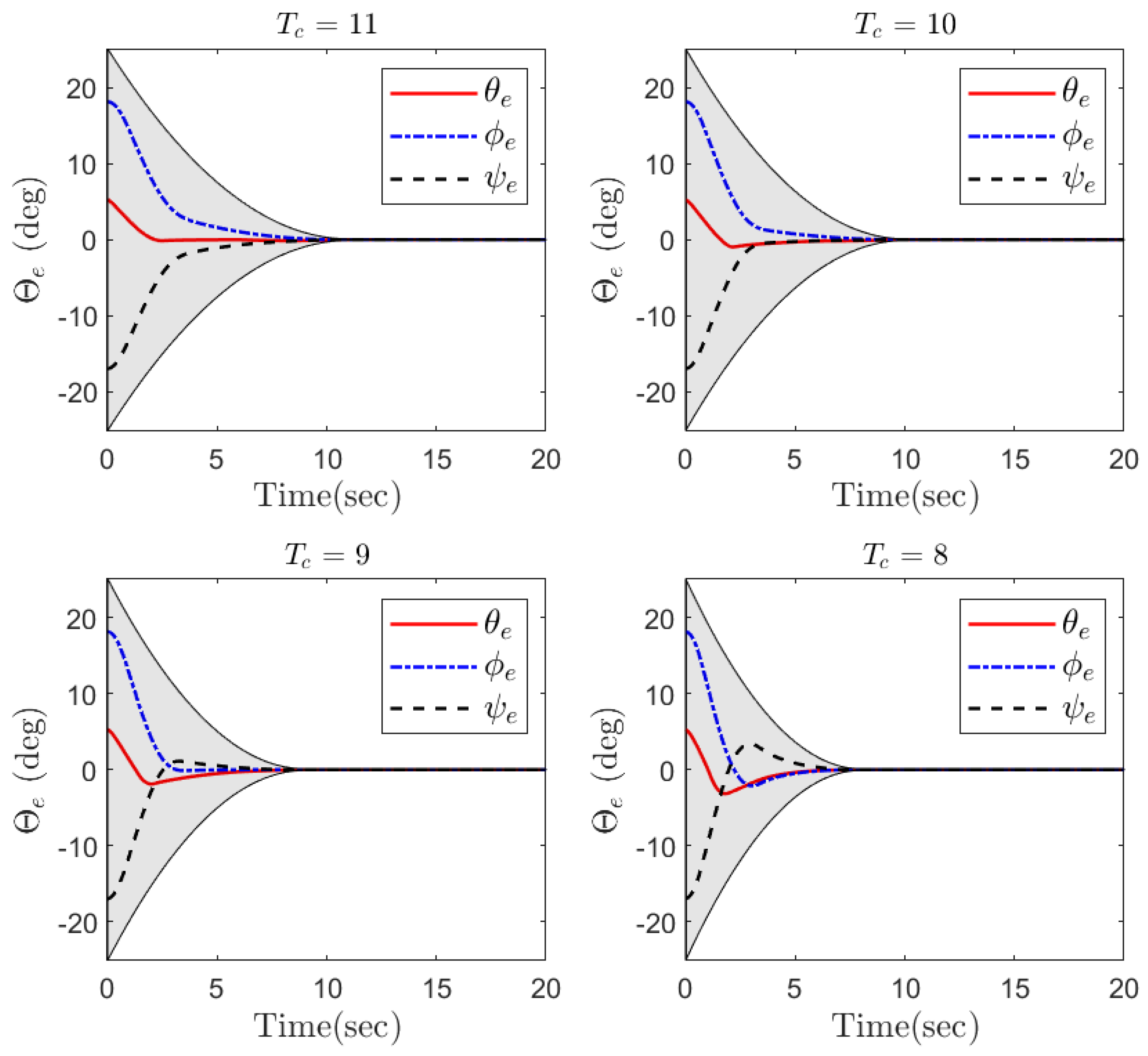
• The predefined performance for the attitude tracking error ${\mathit{x}}_1$ in transient (e.g., maximum overshoot) and steady-state (e.g., ultimate tracking error) settings is specified in advance.

2.3. Preliminaries

Lemma 1. 

Consider the following nonlinear system [37]:

$$\begin{array}{c}\hfill \dot{\mathit{x}}=\mathit{f}(t,\mathit{x},\mathit{d}).\end{array}$$

(7)

Suppose that there exists a positive-definite Lyapunov function $V\left(x\right(t\left)\right)$ satisfying

$$\begin{array}{c}\hfill l\dot{V}\left(x\left(t\right)\right)\le -\frac{\pi }{\eta T_c}\left(V{\left(x\left(t\right)\right)}^{1-\frac{\eta }{2}}+V{\left(x\left(t\right)\right)}^{1+\frac{\eta }{2}}\right),\end{array}$$

where $T_c>0$ and $0<\eta <1$. Then, the origin of the system (7) is prescribed-time stable with specific settling time $T_c$.

Remark 2. 

Based on the concept of the Lyapunov stability [38], if the energy of the nonlinear system (7) denoted by the positive-definite Lyapunov function $V\left(x\right(t\left)\right)$ is nonincreasing, i.e., $\dot{V}\left(x\left(t\right)\right)\le 0$, then the system state $x\left(t\right)$ does not diverge and the system is stable. Moreover, if the condition $\dot{V}\left(x\left(t\right)\right)<0$ is satisfied, then the system is asymptotically stable and the system state $x\left(t\right)$ converges to zero when time tends to infinity. Note that the conventional Lyapunov stability theory guarantees stability of the system over an infinite time horizon. However, Lemma 1 presents a sufficient condition which ensures that the system state $x\left(t\right)$ converges to zero within a finite period of time $T_c$.

Lemma 2. 

Consider the nonlinear system (7) [39]. If the Lyapunov function $V\left(x\right(t\left)\right)$ satisfies the following inequality

$$\begin{array}{c}\hfill \dot{V}\left(x\left(t\right)\right)\le -\frac{\pi }{\eta T_c}\left(V{\left(x\left(t\right)\right)}^{1-\frac{\eta }{2}}+V{\left(x\left(t\right)\right)}^{1+\frac{\eta }{2}}\right)+\delta ,\end{array}$$

where $0<\delta <\infty$, then the system (7) is practically prescribed-time stable where the residual set is expressed as

$$\left\{\underset{t\to T_c^{{}^{\prime }}}{lim}\mathit{x}|V\left(x\left(t\right)\right)\le min\left\{{\left(\frac{2\eta T_c\delta }{\pi }\right)}^{\frac{2}{2-\eta }},{\left(\frac{2\eta T_c\delta }{\pi }\right)}^{\frac{2}{2+\eta }}\right\}\right\}$$

where the parameter $T_c^{{}^{\prime }}$ represents the convergence time such that $T_c^{{}^{\prime }}<\sqrt{2}{T}_c$. Since $0<\eta <1$, then one has $1<\frac{2}{2-\eta }<2$ and $\frac{2}{3}<\frac{2}{2+\eta }<1$. Defining $a={\left(\frac{2\eta T_c\delta }{\pi }\right)}^{\frac{2}{2-\eta }}$ and $b={\left(\frac{2\eta T_c\delta }{\pi }\right)}^{\frac{2}{2+\eta }}$, the value of $\frac{2\eta T_c\delta }{\pi }$ determines whether $a<b$ or $b<a$. To be more exact, if $\frac{2\eta T_c\delta }{\pi }>1$, then $a>b$ and vice versa.

Lemma 3. 

For all $z_i\in {\mathbb{R}}^{+}(i=1,\cdots ,n)$ and $\varsigma >0$, the following inequalities hold [40]:

$$\begin{array}{c}\hfill \left\{\begin{array}{cc}\sum _{i=1}^n{z}_i^{\varsigma }\ge {\left(\sum _{i=1}^n{z}_i\right)}^{\varsigma },\hfill & if0<\varsigma <1\hfill \\ \sum _{i=1}^n{z}_i^{\varsigma }\ge n^{1-\varsigma }{\left(\sum _{i=1}^n{z}_i\right)}^{\varsigma },\hfill & if\varsigma >1.\hfill \end{array}\right.\end{array}$$

(8)

Lemma 4. 

For $z\in \mathbb{R}$ and $\varsigma \ge 0$, one has

$$\begin{array}{c}\hfill 0\le \left|z\right|\le \varsigma +\frac{z^2}{\sqrt{z^2+{\varsigma }^2}}.\end{array}$$

(9)

Definition 1. 

The positive and non-increasing function $\rho \left(t\right)$ is a finite-time prescribed performance function (FTPPF) if ${lim}_{t\to T_f}\rho \left(t\right)={\rho }_T>0$, and $\rho \left(t\right)={\rho }_T$ for any $t\ge T_f$, in which $T_f$ is the required time for the system trajectories to reach the steady-state region and ${\rho }_T$ is the maximum steady-state bound [41].

3. Attitude Control Derivation

3.1. Error Transformation

In order to meet the performance requirements for the attitude tracking error, it is required to guarantee that

$$\begin{array}{c}\hfill -{\rho }_i\left(t\right)<x_{1i}\left(t\right)<{\rho }_i\left(t\right).\end{array}$$

(10)

Indeed, the performance function $\rho \mathbf{\left(}\mathit{t}\mathbf{\right)}={[{\rho }_1\left(t\right),{\rho }_2\left(t\right),{\rho }_3\left(t\right)]}^T$ empowers the designer to specify any favorable performance characteristics for the tracking error in transient (e.g., maximum permitted overshoot) and steady state (e.g., maximum steady-state bound). The function (11) meets the requirements given in Definition 1, and it is utilized as an FTPPF [42,43]

$$\rho \left(t\right)=\left\{\begin{array}{cc}\sqrt[c_1]{{\rho }_0^{c_1}-c_1{c}_{2}t}+{\rho }_T,\hfill & 0\le t<T_f,\hfill \\ {\rho }_T,\hfill & t\ge T_f,\hfill \end{array}\right.$$

(11)

where the positive constants ${\rho }_0$, $c_1$, and $c_2$ are properly selected according to the values of $T_f$, ${\rho }_T$, and $\rho \left(0\right)$. To be more exact, ${\rho }_0=\rho \left(0\right)-{\rho }_T$, $c_2=\frac{{\rho }_0^{c_1}}{c_1{T}_f}$, and $0<c_1=\frac{b_1}{b_2}<1$ such that $b_1$ and $b_2$ are positive odd and even integers, respectively.

An example of the function (11) is provided in Figure 2. Select $\rho \left(0\right)=25$, ${\rho }_T=1$, $T_f=8$, $b_1=5$, and $b_2=10$; then, ${\rho }_0=24$, $c_1=\frac{b_1}{b_2}=0.5$, and $c_2=\frac{{\rho }_0^{c_1}}{c_1{T}_f}=1.22$ are obtained. It can be seen that the function $\rho \left(t\right)$ starts from $\rho \left(0\right)=25$, and at $t=8$ converges to its ultimate value ${\rho }_T=1$ and stays thereafter.

To streamline the design procedure, we define a transformed error variable associated with the tracking error as $\mathit{\lambda }\left(t\right)={[{\lambda }_1\left(t\right),{\lambda }_2\left(t\right),{\lambda }_3\left(t\right)]}^T$ where ${\lambda }_i\left(t\right)=\frac{e_i\left(t\right)}{{\rho }_i\left(t\right)}$. Therefore, the output constraint (10) is equivalent to satisfy $|{\lambda }_i\left(t\right)|<1$ for all $t>0$. Based on the new transformed error, the dynamical system (6) can be rewritten as

$$\begin{array}{c}\hfill \left\{\begin{array}{cc}\dot{\mathit{\lambda }}=\mathrm{diag}\left(\frac{1}{{\rho }_i}\right){\mathit{x}}_2-\mathrm{diag}\left(\frac{\dot{{\rho }_i}}{{\rho }_i}\right)\mathit{\lambda },\hfill & \\ {\dot{\mathit{x}}}_2=\mathbf{\Gamma }-{\mathit{M}}^{-1}{\mathit{R}}^T\mathit{\tau }+{\mathit{M}}^{-1}\mathit{d}.\hfill & \end{array}\right.\end{array}$$

(12)

3.2. Tan-Type BLF Attitude Control Design

In this subsection, a constrained attitude control based on the backstepping control approach is developed. Generally speaking, the backstepping strategy is a recursive procedure interlacing the selection of a Lyapunov function with the design of feedback control. It breaks a design problem for the full system into a sequence of design problems for lower-order (even scalar) subsystems. Moreover, backstepping is able to resolve both stabilization and trajectory tracking control problems under conditions less restrictive than those encountered in other methods, such as sliding mode control, feedback linearization, and gain scheduling [38].

Step 1: Let us construct the following Lyapunov function:

$$\begin{array}{c}\hfill V_1\left(\mathit{\lambda }\right)=\sum _{i=1}^{3}tan\left(\frac{\pi }{2}{\lambda }_i^2\right)\end{array}$$

(13)

where $tan(·)$ represents the tangent function. The Lyapunov function (13) is differentiable in the set $\Omega =\{\lambda \in {\mathbb{R}}^3:|{\lambda }_i|<1,i=1,2,3\}$. The derivative of $V_1\left(\lambda \right)$ gives

$$\begin{array}{c}\hfill {\dot{V}}_1\left(\mathit{\lambda }\right)=\pi \sum _{i=1}^3\frac{{\mathit{\lambda }}^T{\mathbf{{\rm Y}}}_i\dot{\mathit{\lambda }}}{{cos}^2\left({\eta }_i\right)}=\pi \sum _{i=1}^3\frac{{\mathit{\lambda }}^T{\mathbf{{\rm Y}}}_i\left(\mathrm{diag}\left(\frac{1}{{\rho }_i}\right)\mathit{z}+\mathrm{diag}\left(\frac{1}{{\rho }_i}\right)\mathit{\alpha }-\mathrm{diag}\left(\frac{\dot{{\rho }_i}}{{\rho }_i}\right)\mathit{\lambda }\right)}{{cos}^2\left({\eta }_i\right)}\end{array}$$

(14)

where ${\eta }_i=\frac{\pi }{2}{\lambda }_i^2$ and ${\mathbf{{\rm Y}}}_i$ shows a diagonal matrix with consistent dimensions such that the ith diagonal element is the only nonzero element. Further, $\mathit{z}={\mathit{x}}_2-\mathit{\alpha }\in {\mathbb{R}}^3$ denotes the intermediate error, and $\mathit{\alpha }\in {\mathbb{R}}^3$ represents the virtual attitude control expressed by

$$\begin{array}{c}\hfill \mathit{\alpha }=-\frac{1}{\pi }\mathrm{diag}\left({\rho }_i{cos}^2\left({\eta }_i\right)\right)\frac{\overline{\mathit{\alpha }}\left({\mathit{\lambda }}^T\overline{\mathit{\alpha }}\right)}{\sqrt{{\left({\mathit{\lambda }}^T\overline{\mathit{\alpha }}\right)}^2+{\beta }^2}}+\mathrm{diag}\left(\dot{{\rho }_i}\right)\mathit{\lambda }\end{array}$$

(15)

where $\beta \ge 0$ and $\overline{\mathit{\alpha }}={[{\overline{\alpha }}_1,{\overline{\alpha }}_2,{\overline{\alpha }}_3]}^T$ is given by

$$\begin{array}{c}\hfill {\overline{\alpha }}_i=\frac{\pi }{\gamma T_c{\lambda }_i}\left({tan}^{1-\frac{\gamma }{2}}\left({\eta }_i\right)+3^{\gamma }{tan}^{1+\frac{\gamma }{2}}\left({\eta }_i\right)\right)\end{array}$$

(16)

where $0<\gamma <1$ and $T_c$ is the convergence time. By substituting the virtual attitude control (15) into (14), we have

$$\begin{array}{cc}\hfill {\dot{V}}_1\left(\mathit{\lambda }\right)=& \pi \sum _{i=1}^3\frac{{\mathit{\lambda }}^T{\mathbf{{\rm Y}}}_i\mathrm{diag}\left({\rho }_i\right)\mathit{z}}{{cos}^2\left({\eta }_i\right)}+\beta -\left|{\mathit{\lambda }}^T\overline{\mathit{\alpha }}\right|\hfill \\ \hfill \le & \pi \sum _{i=1}^3\frac{{\mathit{\lambda }}^T{\mathbf{{\rm Y}}}_i\mathrm{diag}\left({\rho }_i\right)\mathit{z}}{{cos}^2\left({\eta }_i\right)}+\beta -\frac{\pi }{\gamma T_c}\left(V_1{\left(\mathit{\lambda }\right)}^{1-\frac{\gamma }{2}}+3^{\frac{\gamma }{2}}{V}_1{\left(\mathit{\lambda }\right)}^{1+\frac{\gamma }{2}}\right).\hfill \end{array}$$

(17)

Step 2: Construct an augmented Lyapunov function as

$$\begin{array}{c}\hfill V_2(\mathit{\lambda },\mathit{z})=V_1\left(\mathit{\lambda }\right)+V_z\left(\mathit{z}\right),\end{array}$$

(18)

where $V_z\left(\mathit{z}\right)={\mathit{z}}^T\mathit{z}$. Taking the time derivative of $V_2$ gives

$$\begin{array}{cc}\hfill {\dot{V}}_2(\mathit{\lambda },\mathit{z})=& {\dot{V}}_1\left(\mathit{\lambda }\right)+2{\mathit{z}}^T\dot{\mathit{z}}\hfill \end{array}$$

(19)

where

$$\begin{array}{c}\hfill \dot{\mathit{z}}={\dot{\mathit{x}}}_2-\dot{\mathit{\alpha }}=\mathbf{\Gamma }-{\mathit{M}}^{-1}{\mathit{R}}^T\mathit{\tau }+{\mathit{T}}_d\end{array}$$

(20)

where ${\mathit{T}}_d={\mathit{M}}^{-1}\mathit{d}-\dot{\mathit{\alpha }}$ represents the total disturbance that will be estimated by the disturbance observer.

The actual control input is given by

$$\begin{array}{c}\hfill \mathit{\tau }={\left({\mathit{R}}^T(\mathbf{\Theta })\right)}^{-1}\mathit{M}\left(\frac{\pi }{2}\mathrm{diag}\left(\frac{{\rho }_i}{{cos}^2\left({\eta }_i\right)}\right)\mathit{\lambda }+\frac{\pi }{2\gamma T_c}\left({\mathrm{Sig}}^{1-\gamma }\left(\mathit{z}\right)+3^{\gamma }{\mathrm{Sig}}^{1+\gamma }\left(\mathit{z}\right)\right)+\frac{1}{2}\mathit{z}+\mathbf{\Gamma }+{\widehat{\mathit{T}}}_d\right)\end{array}$$

(21)

where ${\mathrm{Sig}}^{1-\gamma }\left(\mathit{z}\right)={\left[|z_1{|}^{1-\gamma }\mathrm{sgn}\left(z_1\right),|z_2{|}^{1-\gamma }\mathrm{sgn}\left(z_2\right),{\left|z_3\right|}^{1-\gamma }\mathrm{sgn}\left(z_3\right)\right]}^T$ and ${\widehat{\mathit{T}}}_d$ is the estimate of the total disturbance which will be given in the next subsection.

Then, substituting (21) into (19) leads to

$$\begin{array}{cc}\hfill {\dot{V}}_2(\mathit{\lambda },\mathit{z})\le & -\frac{\pi }{\gamma T_c}\left(V_1{\left(\mathit{\lambda }\right)}^{1-\frac{\gamma }{2}}+3^{\frac{\gamma }{2}}{V}_1{\left(\mathit{\lambda }\right)}^{1+\frac{\gamma }{2}}\right)+\beta -{\parallel \mathit{z}\parallel }^2+2{\mathit{z}}^T{\tilde{\mathit{T}}}_d\hfill \\ \hfill & -{\mathit{z}}^T\left(\frac{\pi }{\gamma T_c}\left({\mathrm{Sig}}^{1-\gamma }\left(\mathit{z}\right)+3^{\gamma }{\mathrm{Sig}}^{1+\gamma }\left(\mathit{z}\right)\right)\right)\hfill \\ \hfill \le & -\frac{\pi }{\gamma T_c}\left(V_1{\left(\mathit{\lambda }\right)}^{1-\frac{\gamma }{2}}+3^{\frac{\gamma }{2}}{V}_1{\left(\mathit{\lambda }\right)}^{1+\frac{\gamma }{2}}\right)+\beta -{\parallel \mathit{z}\parallel }^2+2{\mathit{z}}^T{\tilde{\mathit{T}}}_d\hfill \\ \hfill & -\frac{\pi }{\gamma T_c}\left(\sum _{i=1}^3|z_i{|}^{2-\gamma }+3^{\gamma }\sum _{i=1}^3{\left|z_i\right|}^{2+\gamma }\right)\hfill \\ \hfill \le & -\frac{\pi }{\gamma T_c}\left(V_1{\left(\mathit{\lambda }\right)}^{1-\frac{\gamma }{2}}+3^{\frac{\gamma }{2}}{V}_1{\left(\mathit{\lambda }\right)}^{1+\frac{\gamma }{2}}\right)-\frac{\pi }{\gamma T_c}\left(V_z{\left(\mathit{z}\right)}^{1-\frac{\gamma }{2}}+3^{\frac{\gamma }{2}}{V}_z{\left(\mathit{z}\right)}^{1+\frac{\gamma }{2}}\right)\hfill \\ \hfill & +\beta -{\parallel \mathit{z}\parallel }^2+2{\mathit{z}}^T{\tilde{\mathit{T}}}_d\hfill \end{array}$$

(22)

where ${\tilde{\mathit{T}}}_d={\mathit{T}}_d-{\widehat{\mathit{T}}}_d$.

3.3. Disturbance Observer Design

In this part, a predefined-time disturbance observer is developed to accurately estimate the total disturbance ${\mathit{T}}_d$ in Equation (20). The observer guarantees that the estimation error converges to the origin during a pre-specified time regardless of the initial estimation error. Further, this estimation time is explicitly determined as a tunable gain in the observer.

First, let us rewrite Equation (20) as

$$\begin{array}{c}\hfill \dot{\mathit{z}}=-k_1\mathit{z}-{\mathit{M}}^{-1}{\mathit{R}}^T\mathit{\tau }+{\mathit{d}}_{total}\end{array}$$

(23)

where ${\mathit{d}}_{total}=k_1\mathit{z}+\mathbf{\Gamma }+{\mathit{T}}_d$ and $k_1$ is a positive constant. The following auxiliary system is defined to construct an unknown input linear system (UILS) and to use the theoretical concept of unknown input observers [44]:

$$\begin{array}{c}\hfill {\dot{\mathit{z}}}_a=-k_1{\mathit{z}}_a-{\mathit{M}}^{-1}{\mathit{R}}^T\mathit{\tau }.\end{array}$$

(24)

Defining the discrepancy between $\mathit{z}$ and ${\mathit{z}}_a$ by $\mathit{\zeta }=\mathit{z}-{\mathit{z}}_a$; then, the UILS is given by

$$\begin{array}{c}\hfill \left\{\begin{array}{cc}\dot{\mathit{\zeta }}=-k_1\mathit{\zeta }+{\mathit{d}}_{total}\hfill & \\ \mathit{y}=k_2\mathit{\zeta }\hfill & \end{array}\right.\end{array}$$

(25)

where $\mathit{\zeta }$ is the state of the UILS, $\mathit{y}$ is the system output, and $k_2>0$. In the constructed UILS (25), ${\mathit{d}}_{total}$ plays the role of the unknown input, and it will be estimated by the following predefined-time disturbance observer:

$$\begin{array}{c}\hfill \dot{\widehat{\mathit{\zeta }}}=-k_2{k}_3\widehat{\mathit{\zeta }}+\frac{1}{k_2}\dot{\mathit{y}}+k_3\mathit{y}+\frac{k_1^2}{2}{\mathit{\zeta }}_e+\frac{\pi }{2{\gamma }_e{T}_e}\left({\mathrm{Sig}}^{1-{\gamma }_e}\left({\mathit{\zeta }}_e\right)+3^{{\gamma }_e}{\mathrm{Sig}}^{1+{\gamma }_e}\left({\mathit{\zeta }}_e\right)\right)\end{array}$$

(26)

where ${\mathit{\zeta }}_e=\mathit{\zeta }-\widehat{\mathit{\zeta }}$, $k_3>0$, $0<{\gamma }_e<1$, and $T_c$ is the settling time of the observer.

The dynamics of the estimation error can be expressed as

$$\begin{array}{cc}\hfill {\dot{\mathit{\zeta }}}_e=& \dot{\mathit{\zeta }}+k_2{k}_3\widehat{\mathit{\zeta }}-\frac{1}{k_2}\dot{\mathit{y}}-k_3\mathit{y}-\frac{k_1^2}{2}{\mathit{\zeta }}_e-\frac{\pi }{2{\gamma }_e{T}_e}\left({\mathrm{Sig}}^{1-{\gamma }_e}\left({\mathit{\zeta }}_e\right)+3^{{\gamma }_e}{\mathrm{Sig}}^{1+{\gamma }_e}\left({\mathit{\zeta }}_e\right)\right)\hfill \\ \hfill =& -k_2{k}_3{\mathit{\zeta }}_e-\frac{k_1^2}{2}{\mathit{\zeta }}_e-\frac{\pi }{2{\gamma }_e{T}_e}\left({\mathrm{Sig}}^{1-{\gamma }_e}\left({\mathit{\zeta }}_e\right)+3^{{\gamma }_e}{\mathrm{Sig}}^{1+{\gamma }_e}\left({\mathit{\zeta }}_e\right)\right)\hfill \end{array}$$

(27)

Define a continuously differentiable, positive definite Lyapunov function as $V_e\left({\mathit{\zeta }}_e\right)={\mathit{\zeta }}_e^T{\mathit{\zeta }}_e$. The time derivative of $V_e\left({\mathit{\zeta }}_e\right)$ is given as

$$\begin{array}{cc}\hfill {\dot{V}}_e\left({\mathit{\zeta }}_e\right)\le & -\frac{\pi }{{\gamma }_e{T}_e}\left({\mathrm{Sig}}^{1-{\gamma }_e}\left({\mathit{\zeta }}_e\right)+3^{{\gamma }_e}{\mathrm{Sig}}^{1+{\gamma }_e}\left({\mathit{\zeta }}_e\right)\right)-k_1^2{\parallel {\mathit{\zeta }}_e\parallel }^2\hfill \\ \hfill \le & -\frac{\pi }{{\gamma }_e{T}_e}\left(V_e{\left({\mathit{\zeta }}_e\right)}^{1-\frac{{\gamma }_e}{2}}+3^{\frac{{\gamma }_e}{2}}{V}_e{\left({\mathit{\zeta }}_e\right)}^{1+\frac{{\gamma }_e}{2}}\right)-k_1^2{\parallel {\mathit{\zeta }}_e\parallel }^2.\hfill \end{array}$$

(28)

The inequality (28) can be rewritten as

$$\begin{array}{c}\hfill {\dot{V}}_e\left({\mathit{\zeta }}_e\right)=\frac{d{V}_e\left({\mathit{\zeta }}_e\right)}{dt}=-\frac{\pi }{{\gamma }_e{T}_e}\left(V_e{\left({\mathit{\zeta }}_e\right)}^{1-\frac{{\gamma }_e}{2}}+V_e{\left({\mathit{\zeta }}_e\right)}^{1+\frac{{\gamma }_e}{2}}\right)+\epsilon ,\end{array}$$

(29)

where $\epsilon$ is a nonnegative constant. Solving the above differential equation gives

$$\begin{array}{c}\hfill T\left({\mathit{\zeta }}_{e0}\right)=-{\int }_{V_e\left({\mathit{\zeta }}_{e0}\right)}^0\frac{d{V}_e\left({\mathit{\zeta }}_e\right)}{\frac{\pi }{{\gamma }_e{T}_e}\left(V_e{\left({\mathit{\zeta }}_e\right)}^{1-\frac{{\gamma }_e}{2}}+V_e{\left({\mathit{\zeta }}_e\right)}^{1+\frac{{\gamma }_e}{2}}\right)+\epsilon }\le \frac{{\gamma }_e{T}_e}{\pi }{\int }_0^{V_e\left({\mathit{\zeta }}_{e0}\right)}\frac{d{V}_e}{V_e{\left({\mathit{\zeta }}_e\right)}^{1-\frac{{\gamma }_e}{2}}+V_e{\left({\mathit{\zeta }}_e\right)}^{1+\frac{{\gamma }_e}{2}}}.\end{array}$$

(30)

Therefore, one can obtain

$$\begin{array}{c}\hfill T\left({\mathit{\zeta }}_{e0}\right)\le T_e\left(\frac{2}{\pi }arctan(V_e{\left({\mathit{\zeta }}_{e0}\right)}^{\frac{{\gamma }_e}{2}}\right).\end{array}$$

(31)

It should be noted that $T\left({\mathit{\zeta }}_{e0}\right)\le T_e$ and $T_e={lim}_{V_e\left({\mathit{\zeta }}_{\mathbf{e}\mathbf{0}}\right)\to \infty }T\left({\mathit{\zeta }}_{e0}\right)$. This confirms that even if the initial estimation error tends to infinity, the convergence time does exceed $T_e$.

Then, the unknown input ${\mathit{d}}_{total}$ is estimated by ${\widehat{\mathit{d}}}_{total}$ within a predefined time $T_e$ as

$$\begin{array}{c}\hfill {\widehat{\mathit{d}}}_{total}=k_1\widehat{\mathit{\zeta }}+\frac{1}{k_2}\dot{\mathit{y}}.\end{array}$$

(32)

Based on ${\widehat{\mathit{d}}}_{total}$, the total disturbance ${\mathit{T}}_d$ is reconstructed by

$$\begin{array}{c}\hfill {\widehat{\mathit{T}}}_d={\widehat{\mathit{d}}}_{total}-k_1\mathit{z}-\mathbf{\Gamma }.\end{array}$$

(33)

By defining ${\tilde{\mathit{T}}}_d={\mathit{T}}_d-{\widehat{\mathit{T}}}_d$ and using Equation (33), one has

$$\begin{array}{cc}\hfill {\tilde{\mathit{T}}}_d=& {\mathit{d}}_{total}-k_1\mathit{z}-\mathbf{\Gamma }-{\widehat{\mathit{d}}}_{total}+k_1\mathit{z}+\mathbf{\Gamma }={\mathit{d}}_{total}-k_1\widehat{\mathit{\zeta }}-\frac{1}{k_2}\dot{\mathit{y}}\hfill \\ \hfill =& {\mathit{d}}_{total}-k_1\widehat{\mathit{\zeta }}-\frac{1}{k_2}\left(-k_1{k}_2\mathit{\zeta }+k_2{\mathit{d}}_{total}\right)=k_1{\mathit{\zeta }}_e\hfill \end{array}$$

(34)

3.4. Stability Analysis

The predefined-time stability of the closed-loop attitude system in the presence of the controller and the observer is established via the following theorem.

Theorem 1. 

Consider the uncertain spacecraft attitude system (6). If the disturbance observer and the controller are, respectively, designed as Equations (26) and (21), then the attitude tracking maneuver is accomplished within a predefined time $T_c$, and the constraint on the attitude tracking error ${\mathit{x}}_1$ is satisfied.

Proof. 

Define the final Lyapunov function as

$$\begin{array}{c}\hfill V_f(\mathit{\lambda },\mathit{z},{\mathit{\zeta }}_e)=V_1\left(\mathit{\lambda }\right)+V_z\left(\mathit{z}\right)+V_e\left({\mathit{\zeta }}_e\right).\end{array}$$

(35)

Differentiating $V_f(\mathit{\lambda },\mathit{z},{\mathit{\zeta }}_e)$ with respect to time and using Equations (22) and (28), one has

$$\begin{array}{cc}\hfill {\dot{V}}_f(\mathit{\lambda },\mathit{z},{\mathit{\zeta }}_e)\le & -\frac{\pi }{\gamma T_c}\left(V_1{\left(\mathit{\lambda }\right)}^{1-\frac{\gamma }{2}}+3^{\frac{\gamma }{2}}{V}_1{\left(\mathit{\lambda }\right)}^{1+\frac{\gamma }{2}}\right)-\frac{\pi }{\gamma T_c}\left(V_z{\left(\mathit{z}\right)}^{1-\frac{\gamma }{2}}+3^{\frac{\gamma }{2}}{V}_z{\left(\mathit{z}\right)}^{1+\frac{\gamma }{2}}\right)\hfill \\ \hfill & -\frac{\pi }{{\gamma }_e{T}_e}\left(V_e{\left({\mathit{\zeta }}_e\right)}^{1-\frac{{\gamma }_e}{2}}+3^{\frac{{\gamma }_e}{2}}{V}_e{\left({\mathit{\zeta }}_e\right)}^{1+\frac{{\gamma }_e}{2}}\right)+2{\mathit{z}}^T{\tilde{\mathit{T}}}_d+\beta -{\parallel \mathit{z}\parallel }^2-k_1^2{\parallel {\mathit{\zeta }}_e\parallel }^2\hfill \end{array}$$

(36)

From Equation (34), it is observed that ${\tilde{\mathit{T}}}_d=k_1{\mathit{\zeta }}_e$. Then, according to Young’s inequality, one has

$$\begin{array}{c}\hfill 2{\mathit{z}}^T{\tilde{\mathit{T}}}_d\le {\parallel \mathit{z}\parallel }^2+k_1^2{\parallel {\mathit{\zeta }}_e\parallel }^2.\end{array}$$

(37)

Then, the inequality (36) is simplified as

$$\begin{array}{cc}\hfill {\dot{V}}_f(\mathit{\lambda },\mathit{z},{\mathit{\zeta }}_e)& \le -\frac{\pi }{\gamma T_c}\left(V_1{\left(\mathit{\lambda }\right)}^{1-\frac{\gamma }{2}}+3^{\frac{\gamma }{2}}{V}_1{\left(\mathit{\lambda }\right)}^{1+\frac{\gamma }{2}}\right)-\frac{\pi }{\gamma T_c}\left(V_z{\left(\mathit{z}\right)}^{1-\frac{\gamma }{2}}+3^{\frac{\gamma }{2}}{V}_z{\left(\mathit{z}\right)}^{1+\frac{\gamma }{2}}\right)\hfill \\ & -\frac{\pi }{{\gamma }_e{T}_e}\left(V_e{\left({\mathit{\zeta }}_e\right)}^{1-\frac{{\gamma }_e}{2}}+3^{\frac{{\gamma }_e}{2}}{V}_e{\left({\mathit{\zeta }}_e\right)}^{1+\frac{{\gamma }_e}{2}}\right)+\beta \hfill \end{array}$$

(38)

Select ${\gamma }_e=\gamma$. Since the settling time of the observer (i.e., $T_e$) should be adequately smaller than that of the controller (i.e., $T_c$), we have $T_e<T_c$. Hence, (38) should be rewritten as

$$\begin{array}{cc}\hfill {\dot{V}}_f(\mathit{\lambda },\mathit{z},{\mathit{\zeta }}_e)\le & -\frac{\pi }{\gamma T_c}\left(V_f{(\mathit{\lambda },\mathit{z},{\mathit{\zeta }}_e)}^{1-\frac{\gamma }{2}}+V_f{(\mathit{\lambda },\mathit{z},{\mathit{\zeta }}_e)}^{1+\frac{\gamma }{2}}\right)+\beta .\hfill \end{array}$$

(39)

Based on Lemma 2, it can be concluded that the closed-loop attitude system is predefined-time stable and the reference trajectory is tracked during a fixed time while the constrained on the error trajectory is satisfied. This completes the proof. □

Remark 3. 

The derivative of the virtual control (15) is given as

$$\begin{array}{c}\hfill {\dot{\alpha }}_i=-\frac{{\dot{\rho }}_i}{\pi }{cos}^2\left(\frac{\pi }{2}{\lambda }_i^2\right){\Psi }_i+{\rho }_i{\lambda }_i{\dot{\lambda }}_{i}sin\left(\pi {\lambda }_i^2\right){\Psi }_i-\frac{{\rho }_i}{\pi }{cos}^2\left(\frac{\pi }{2}{\lambda }_i^2\right){\dot{\Psi }}_i+{\ddot{\rho }}_i{\lambda }_i+{\dot{\rho }}_i{\dot{\lambda }}_i\end{array}$$

(40)

where

$${\Psi }_i=\frac{{\overline{\alpha }}_i\left({\lambda }_i{\overline{\alpha }}_i\right)}{\sqrt{{\left({\lambda }_i{\overline{\alpha }}_i\right)}^2+{\beta }^2}},{\dot{\Psi }}_i=\frac{\frac{d}{dt}\left({\overline{\alpha }}_i\left({\lambda }_i{\overline{\alpha }}_i\right)\right)\sqrt{{\left({\lambda }_i{\overline{\alpha }}_i\right)}^2+{\beta }^2}-{\overline{\alpha }}_i\left({\lambda }_i{\overline{\alpha }}_i\right)\frac{d}{dt}\left(\sqrt{{\left({\lambda }_i{\overline{\alpha }}_i\right)}^2+{\beta }^2}\right)}{{\left({\lambda }_i{\overline{\alpha }}_i\right)}^2+{\beta }^2},$$

and

$$\frac{d}{dt}\left({\overline{\alpha }}_i\left({\lambda }_i{\overline{\alpha }}_i\right)\right)={\dot{\overline{\alpha }}}_i\left({\lambda }_i{\overline{\alpha }}_i\right)+{\overline{\alpha }}_i\left({\dot{\lambda }}_i{\overline{\alpha }}_i\right)+{\overline{\alpha }}_i\left({\lambda }_i{\dot{\overline{\alpha }}}_i\right),$$

$$\frac{d}{dt}\left(\sqrt{{\left({\lambda }_i{\overline{\alpha }}_i\right)}^2+{\beta }^2}\right)=\frac{\dot{{\lambda }_i}{\overline{\alpha }}_i\left({\lambda }_i{\overline{\alpha }}_i\right)+{\lambda }_i{\dot{\overline{\alpha }}}_i\left({\lambda }_i{\overline{\alpha }}_i\right)+{\lambda }_i{\overline{\alpha }}_i\left({\dot{\lambda }}_i{\overline{\alpha }}_i\right)+{\lambda }_i{\overline{\alpha }}_i\left({\lambda }_i{\dot{\overline{\alpha }}}_i\right)}{2\sqrt{{\left({\lambda }_i{\overline{\alpha }}_i\right)}^2+{\beta }^2}},$$

$$\begin{array}{cc}\hfill {\dot{\overline{\alpha }}}_i=\frac{\pi }{\gamma T_c}(& \frac{{sec}^2\left(\frac{\pi }{2}{\lambda }_i^2\right)\left(2(1-\frac{\gamma }{2})\pi {\lambda }_i^2-sin\left(\pi {\lambda }_i^2\right)\right){tan}^{-\frac{\gamma }{2}}\left(\frac{\pi }{2}{\lambda }_i^2\right)}{2{\lambda }_i^2}\hfill \\ & +3^{\gamma }{tan}^{\frac{\gamma }{2}}\left(\frac{\pi }{2}{\lambda }_i^2\right)\left(\pi (1+\frac{\gamma }{2}){sec}^2\left(\frac{\pi }{2}{\lambda }_i^2\right)-\frac{tan\left(\frac{\pi }{2}{\lambda }_i^2\right)}{{\lambda }_i^2}\right)){\dot{\lambda }}_i.\hfill \end{array}$$

(41)

Thus, Equation (40) can be rewritten as

$$\begin{array}{cc}\hfill {\dot{\alpha }}_i=& -\frac{{\dot{\rho }}_i}{\pi }{cos}^2\left(\frac{\pi }{2}{\lambda }_i^2\right)\frac{{\overline{\alpha }}_i\left({\lambda }_i{\overline{\alpha }}_i\right)}{\sqrt{{\left({\lambda }_i{\overline{\alpha }}_i\right)}^2+{\beta }^2}}+{\rho }_i{\lambda }_i{\dot{\lambda }}_{i}sin\left(\pi {\lambda }_i^2\right)\frac{{\overline{\alpha }}_i\left({\lambda }_i{\overline{\alpha }}_i\right)}{\sqrt{{\left({\lambda }_i{\overline{\alpha }}_i\right)}^2+{\beta }^2}}+{\ddot{\rho }}_i{\lambda }_i+{\dot{\rho }}_i{\dot{\lambda }}_i\hfill \\ \hfill & -\frac{{\rho }_i}{\pi }{cos}^2\left(\frac{\pi }{2}{\lambda }_i^2\right)\frac{\left({\dot{\overline{\alpha }}}_i\left({\lambda }_i{\overline{\alpha }}_i\right)+{\overline{\alpha }}_i\left({\dot{\lambda }}_i{\overline{\alpha }}_i\right)+{\overline{\alpha }}_i\left({\lambda }_i{\dot{\overline{\alpha }}}_i\right)\right)\sqrt{{\left({\lambda }_i{\overline{\alpha }}_i\right)}^2+{\beta }^2}}{{\left({\lambda }_i{\overline{\alpha }}_i\right)}^2+{\beta }^2}\hfill \\ \hfill & +\frac{{\rho }_i}{\pi }{cos}^2\left(\frac{\pi }{2}{\lambda }_i^2\right)\frac{{\overline{\alpha }}_i\left({\lambda }_i{\overline{\alpha }}_i\right)\left(\dot{{\lambda }_i}{\overline{\alpha }}_i\left({\lambda }_i{\overline{\alpha }}_i\right)+{\lambda }_i{\dot{\overline{\alpha }}}_i\left({\lambda }_i{\overline{\alpha }}_i\right)+{\lambda }_i{\overline{\alpha }}_i\left({\dot{\lambda }}_i{\overline{\alpha }}_i\right)+{\lambda }_i{\overline{\alpha }}_i\left({\lambda }_i{\dot{\overline{\alpha }}}_i\right)\right)}{2{({\left({\lambda }_i{\overline{\alpha }}_i\right)}^2+{\beta }^2)}^{\frac{3}{2}}}.\hfill \end{array}$$

(42)

If the conventional backstepping method is used, the virtual attitude control would be designed as

$$\mathit{\alpha }=-\frac{1}{\pi }\mathrm{diag}\left({\rho }_i{cos}^2\left({\eta }_i\right)\right)\overline{\mathit{\alpha }}+\mathrm{diag}\left(\dot{{\rho }_i}\right)\mathit{\lambda }.$$

Then, based on Equation (41), the singularity issue can happen in $\dot{\mathit{\alpha }}$ because of $0<\gamma <1$ when ${\lambda }_i=0$. However, the time derivative of the proposed virtual attitude control Equation (15) contains the term $\frac{{\rho }_i}{\pi }{cos}^2\left(\frac{\pi }{2}{\lambda }_i^2\right){\lambda }_i{\alpha }_i{\dot{\overline{\alpha }}}_i$, and consequently, the singularity is directly removed.

Remark 4. 

The diagram of the proposed control framework constituting the rigid spacecraft, the observer, and the controller is presented in Figure 3.

To sum up, a disturbance-observer-based attitude tracking control for a rigid spacecraft was developed in this section. A nonsingular fixed-time backstepping control is designed to guarantee that the system states converge to a small region around the origin within a predefined time $T_c$ and the singularity will never happen. The proposed observer estimates the total uncertainty in a fixed time $T_e$, and the estimated signal is used as a feed-forward control method in the main controller.

4. Simulation Results

A numerical simulation was conducted on a rigid spacecraft to validate the efficacy of the proposed predefined-time constrained control framework. The nominal inertia matrix is ${\mathit{J}}_0=\left[\begin{array}{ccc}35& 2& -4\\ 2& 40& -3\\ -4& -3& 38\end{array}\right]$$\mathrm{kg}·{\mathrm{m}}^2$. It is assumed that the inertia matrix uncertainty is given as $\Delta \mathit{J}=\left\{\begin{array}{cc}-(1.2+exp(-0.2t)){\mathit{J}}_v,\hfill & t<2\hfill \\ -(1.2+exp(-0.2t)+1.5){\mathit{J}}_v,\hfill & t\ge 2\hfill \end{array}\right.$ with ${\mathit{J}}_v=\mathrm{diag}[3.5,2,1.8]$ $\mathrm{kg}·{\mathrm{m}}^2$. The constant term $1.5{\mathit{J}}_v$ can be regarded as fuel leakage. In addition to the inertia uncertainty, we suppose the following environmental disturbance acts on the spacecraft: ${\mathit{\tau }}_d=\left({\parallel \omega \parallel }^2+0.025\right){[sin\left(0.08t\right),-cos\left(0.04t\right),sin\left(0.06t\right)]}^T+\delta (t-6){[2,1,1.5]}^T$$\mathrm{N}·\mathrm{m}$ in which $\delta (·)$ is a unit step. The second term of the considered disturbance can result from connecting with a space debris. Taking high-resolution images of the areas of interest is an important task for the considered spacecraft. To do this, the spacecraft should accomplish fast and an accurate attitude tracking maneuver with the reference attitude trajectory as ${\mathbf{\Theta }}_d={[-30sin(0.05t-\pi /10),20cos(0.02t-\pi /4),30sin(0.01t-\pi /6)]}^T$ degree. The parameters of the proposed controller and observer were selected as $\gamma =5/9$, $T_c=8$, $\beta =0.01$, ${\rho }_0=25$, ${\rho }_T=0.1$, $c_1=0.5$, $T_f=8$, $k_1=1$, $k_2=1$, $k_3=1$, ${\gamma }_e=5/9$, and $T_e=0.1$.

Part 1: In this part, four different initial conditions are considered. The main objective is to show that the convergence time of the closed-loop system does not depend on the initial conditions and the system trajectories are stabilized within $T_c$. The four initial conditions were: (1) $\mathbf{\Theta }\left(0\right)={[5,-4,-10]}^T$ deg and $\mathit{\omega }\left(0\right)={[0,0.1,-0.1]}^T$ deg/s, (2) $\mathbf{\Theta }\left(0\right)={[7,-3,4]}^T$ deg and $\mathit{\omega }\left(0\right)={[-0.15,0.15,-0.15]}^T$ deg/s, (3) $\mathbf{\Theta }\left(0\right)={[-5,-5,0]}^T$ deg and $\mathit{\omega }\left(0\right)={[-0.25,-0.25,0.2]}^T$ deg/s, and (4) $\mathbf{\Theta }\left(0\right)={[6,-5,7]}^T$ deg and $\mathit{\omega }\left(0\right)={[0.15,-0.25,-0.15]}^T$ deg/s. The simulation results associated with this part are illustrated in Figure 4, Figure 5, Figure 6 and Figure 7. In Figure 4, the attitude and angular tracking error trajectories are stabilized before 8 s which is less than the upper bound of the convergence time, i.e., $T_c$. This is true for all the initial conditions and confirms the claim that the trajectories are stabilized before $T_c$ for any given initial condition. Further, the prescribed performance for the attitude tracking error was achieved regardless of the initial conditions. According to Figure 6, it can be observed that when the attitude tracking error approaches the performance function (i.e., $x_{1i}\to {\rho }_i$), the function ${\lambda }_i$ tends to 1, and consequently, the tan function increases. In Figure 7, when the attitude tracking error trajectory is going to contact the boundary of the allowed region, the control input increases to preclude it from violating the constraint.

Part 2: The main control objective was to assess how the controller forces the system’s trajectories to converge to zero if there are different convergence times. To this end, the initial conditions were taken as $\mathbf{\Theta }\left(0\right)={[4,-4,2]}^T$ deg and $\mathit{\omega }\left(0\right)={[0.18,0.22,-0.22]}^T$ deg/s. The parameters of the observer and the controller were the same as the previous part except for $T_c$ and $T_f$. Four different cases were taken into account. (1) $T_c=T_f=11$, (2) $T_c=T_f=10$, (3) $T_c=T_f=9$, and (4) $T_c=T_f=8$. Based on Figure 8 and Figure 9, smaller values of $T_c$ and $T_f$ will lead to faster convergence. Obviously, even when the convergence time becomes smaller, the prescribed performance for the attitude tracking error is still satisfied. This, in turn, confirms that the suggested control scheme is capable of stabilizing the system before a predefined time without violating the constraints on the tracking error. However, as is shown in Figure 10, when the convergence time becomes smaller, the time-varying gain $\lambda$ rises, and it may approach 1. Consequently, the required control effort, depicted in Figure 11, increases. Due to the importance of control energy in practical applications, a compromise between the convergence rate and the required control effort should be made.

Part 3: In this part, the proposed control scheme is compared with the disturbance-observer-based predefined-time attitude tracking control (DOBPTATC) [20] and the robust fixed-time attitude control (RFTAC) in [19]. The DOBPTATC and the RFTAC are disturbance-observer-based attitude tracking controls with fixed-time convergence for rigid spacecraft. Thus, they can be appropriate for comparison. The initial conditions, the inertia uncertainty, the environmental disturbances, and the reference trajectory are considered the ones presented in [20].

The attitude and rotation velocity tracking errors are depicted in Figure 12 and Figure 13, respectively. It is shown that the proposed controller results in much faster convergence with reduced settling time. To be more exact, the error trajectories under the proposed controller, the RFTAC, and the DOBPTATC were stabilized after roughly 8, 14, and 19 s, respectively. This means that the proposed approach reduces the convergence time by $42.8\%$ and $57.9\%$ with respect to the RFTAC and the DOBPTATC. Further, in contrast to the RFTAC and the DOBPTATC, the proposed control method is capable of providing desirable performance in transient and steady states for the attitude tracking error. Although the proposed control method achieved superior performance to RFTAC and the DOBPTATC, the required initial control efforts for the three controllers were approximately the same. This fact can be clearly observed in Figure 14. Therefore, the new control framework guarantees much better performance without having to consume extra control energy. The estimation error is depicted in Figure 15. As expected, the estimation error quickly converged to zero within a predefined time $T_e$. Although there are two discontinuities in the total disturbance at $t=2$ and $t=6$, the proposed observer was still able to stabilize the estimation error and made it converge to zero rapidly. Further, the total disturbance, along with its estimation, is illustrated in Figure 16. This figure clearly shows that the total disturbance was precisely reconstructed by the proposed observer.

To further analyze the performance of the proposed control scheme in comparison with the RFTAC and the DOBPTATC, the convergence time and the steady-state tracking error under the three control laws have been tabulated in

Table 1. Performance comparison with different controllers.

Controller	$|{\mathbf{\Theta }}_{\mathit{e}\mathit{i}}|$ in Steady-State	$|{\mathit{\omega }}_{\mathit{e}\mathit{i}}|$ in  Steady-State	Settling Time
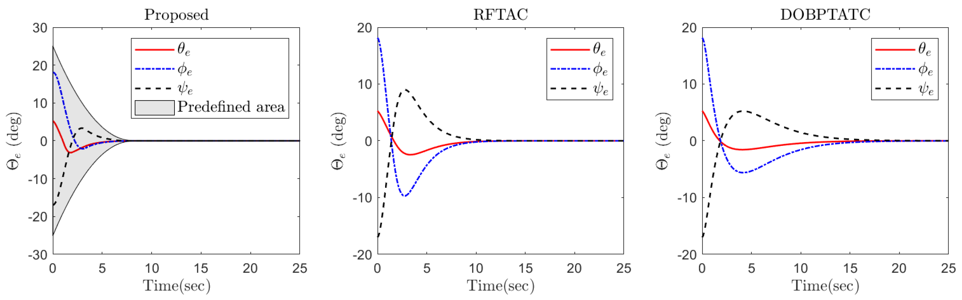
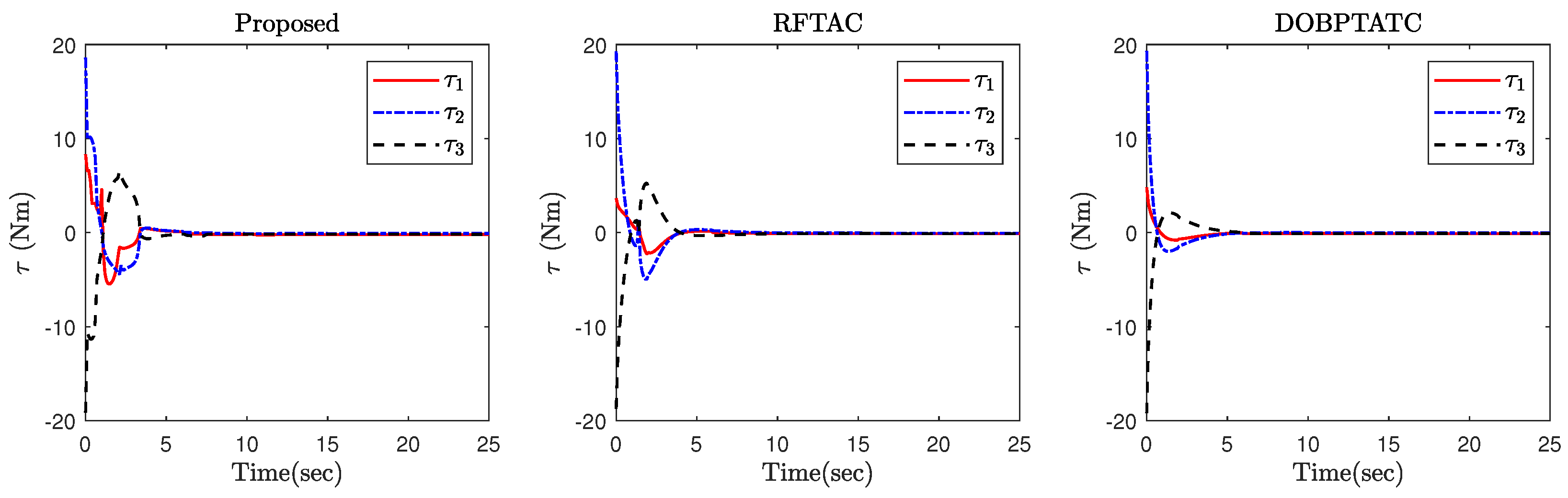
Proposed	$3.3\times {10}^{-7}$	$5.7\times {10}^{-7}$	$7.9$
RFTAC	$1.5\times {10}^{-6}$	$1.9\times {10}^{-6}$	$14.3$
DOBPTATC	$1.4\times {10}^{-6}$	$1.6\times {10}^{-6}$	$19.1$

. In this table, the settling time shows the time when the attitude tracking error enters the region $|{\mathbf{\Theta }}_{ei}|<{10}^{-3}$ and stays thereafter. It can be observed that the proposed control scheme improves the convergence rate by reducing the settling time, the point accuracy through decreasing the $|{\mathbf{\Theta }}_{ei}|$, and point stability by reducing $|{\mathit{\omega }}_{ei}|$, simultaneously. Therefore, the simulation results confirm the superior performance of the proposed control framework in accomplishing the attitude tracking maneuver for the spacecraft.

To sum up, the simulation results verify the claim provided in Theorem 1 and illustrate the superiority of the proposed control scheme over the RFTAC and the DOBPTATC.

5. Conclusions

This work investigated the problem of disturbance-observer-based attitude tracking control design for spacecraft in spite of uncertainty and arbitrary disturbance. By virtue of the backstepping control, a nonsingular attitude tracking control with predefined settling time and performance was developed. More specifically, a quadratic function is employed in the virtual control scheme to resolve the problem of a singularity without employing any command filter or piece-wise continuous function. Moreover, a tan-type BLF-based control method was designed such that the constraint on the attitude is satisfied and the closed-loop system is practically predefined-time stable. The lowest upper bound of the convergence time was determined as an independent gain in the controller. Further, a disturbance observer with predefined-time stability was designed to precisely reconstruct the total disturbance of the system. Various simulation results show the efficiency and applicability of the suggested control framework.

References

- Yao, Q.; Jahanshahi, H.; Bekiros, S.; Mihalache, S.F.; Alotaibi, N.D. Indirect Neural-Enhanced Integral Sliding Mode Control for Finite-Time Fault-Tolerant Attitude Tracking of Spacecraft. Mathematics 2022, 10, 2467. [Google Scholar] [CrossRef]
- Dai, M.Z.; Xiao, B.; Zhang, C.; Wu, J. Event-triggered policy to spacecraft attitude stabilization with actuator output nonlinearities. IEEE Trans. Circuits Syst. II Express Briefs 2021, 68, 2855–2859. [Google Scholar] [CrossRef]
- Chen, W.; Hu, Q. Sliding-mode-based attitude tracking control of spacecraft under reaction wheel uncertainties. IEEE/CAA J. Autom. Sin. 2022, 1–13. [Google Scholar] [CrossRef]
- Yao, Q. Robust finite-time control design for attitude stabilization of spacecraft under measurement uncertainties. Adv. Space Res. 2021, 68, 3159–3175. [Google Scholar] [CrossRef]
- Shang, D.; Li, X.; Yin, M.; Li, F. Vibration Suppression for Two-Inertia System With Variable-Length Flexible Load Based on Neural Network Compensation Sliding Mode Controller and Angle-Independent Method. IEEE/ASME Trans. Mechatron. 2022, 1–12. [Google Scholar] [CrossRef]
- Shang, D.; Li, X.; Yin, M.; Li, F. Dynamic modeling and control for dual-flexible servo system considering two-dimensional deformation based on neural network compensation. Mech. Mach. Theory 2022, 175, 104954. [Google Scholar] [CrossRef]
- Shang, D.; Li, X.; Yin, M.; Li, F. Tracking control strategy for space flexible manipulator considering nonlinear friction torque based on adaptive fuzzy compensation sliding mode controller. Adv. Space Res. 2022. [Google Scholar] [CrossRef]
- Yao, Q.; Jahanshahi, H.; Moroz, I.; Alotaibi, N.D.; Bekiros, S. Neural Adaptive Fixed-Time Attitude Stabilization and Vibration Suppression of Flexible Spacecraft. Mathematics 2022, 10, 1667. [Google Scholar] [CrossRef]
- Golestani, M.; Mobayen, S.; ud Din, S.; El-Sousy, F.F.; Vu, M.T.; Assawinchaichote, W. Prescribed performance attitude stabilization of a rigid body under physical limitations. IEEE Trans. Aerosp. Electron. Syst. 2022, 58, 4147–4155. [Google Scholar] [CrossRef]
- Hu, Q.; Tan, X. Dynamic near-optimal control allocation for spacecraft attitude control using a hybrid configuration of actuators. IEEE Trans. Aerosp. Electron. Syst. 2019, 56, 1430–1443. [Google Scholar] [CrossRef]
- Liu, Y.; Jiang, B.; Lu, J.; Cao, J.; Lu, G. Event-triggered sliding mode control for attitude stabilization of a rigid spacecraft. IEEE Trans. Syst. Man Cybern. Syst. 2018, 50, 3290–3299. [Google Scholar] [CrossRef]
- Li, H.; Yan, W.; Shi, Y. Continuous-time model predictive control of under-actuated spacecraft with bounded control torques. Automatica 2017, 75, 144–153. [Google Scholar] [CrossRef]
- Fridman, L.; Levant, A.; Davila, J. Observation of linear systems with unknown inputs via high-order sliding-modes. Int. J. Syst. Sci. 2007, 38, 773–791. [Google Scholar] [CrossRef]
- Sanyal, A.; Fosbury, A.; Chaturvedi, N.; Bernstein, D.S. Inertia-free spacecraft attitude tracking with disturbance rejection and almost global stabilization. J. Guid. Control Dyn. 2009, 32, 1167–1178. [Google Scholar] [CrossRef] [Green Version]
- Weiss, A.; Kolmanovsky, I.; Bernstein, D.S.; Sanyal, A. Inertia-free spacecraft attitude control using reaction wheels. J. Guid. Control Dyn. 2013, 36, 1425–1439. [Google Scholar] [CrossRef] [Green Version]
- Bai, Y.; Biggs, J.D.; Zazzera, F.B.; Cui, N. Adaptive attitude tracking with active uncertainty rejection. J. Guid. Control Dyn. 2018, 41, 550–558. [Google Scholar] [CrossRef]
- Sun, L.; Zheng, Z. Disturbance-observer-based robust backstepping attitude stabilization of spacecraft under input saturation and measurement uncertainty. IEEE Trans. Ind. Electron. 2017, 64, 7994–8002. [Google Scholar] [CrossRef]
- Xiao, B.; Cao, L.; Xu, S.; Liu, L. Robust tracking control of robot manipulators with actuator faults and joint velocity measurement uncertainty. IEEE/ASME Trans. Mechatron. 2020, 25, 1354–1365. [Google Scholar] [CrossRef]
- Cao, L.; Xiao, B.; Golestani, M. Robust fixed-time attitude stabilization control of flexible spacecraft with actuator uncertainty. Nonlinear Dyn. 2020, 100, 2505–2519. [Google Scholar] [CrossRef]
- Xiao, B.; Wu, X.; Cao, L.; Hu, X. Prescribed Time Attitude Tracking Control of Spacecraft with Arbitrary Disturbance. IEEE Trans. Aerosp. Electron. Syst. 2022, 58, 2531–2540. [Google Scholar] [CrossRef]
- Xia, K.; Zou, Y. Adaptive fixed-time fault-tolerant control for noncooperative spacecraft proximity using relative motion information. Nonlinear Dyn. 2020, 100, 2521–2535. [Google Scholar] [CrossRef]
- Du, H.; Zhang, J.; Wu, D.; Zhu, W.; Li, H.; Chu, Z. Fixed-time attitude stabilization for a rigid spacecraft. ISA Trans. 2020, 98, 263–270. [Google Scholar] [CrossRef] [PubMed]
- Zou, A.M.; Kumar, K.D.; de Ruiter, A.H. Fixed-time attitude tracking control for rigid spacecraft. Automatica 2020, 113, 108792. [Google Scholar] [CrossRef]
- Zou, A.M.; Fan, Z. Fixed-time attitude tracking control for rigid spacecraft without angular velocity measurements. IEEE Trans. Ind. Electron. 2020, 67, 6795–6805. [Google Scholar] [CrossRef]
- Shi, X.N.; Zhou, Z.G.; Zhou, D. Adaptive Fault-Tolerant Attitude Tracking Control of Rigid Spacecraft on Lie Group with Fixed-Time Convergence. Asian J. Control 2020, 22, 423–435. [Google Scholar] [CrossRef]
- Cruz-Ortiz, D.; Chairez, I.; Poznyak, A. Non-singular terminal sliding-mode control for a manipulator robot using a barrier Lyapunov function. ISA Trans. 2022, 121, 268–283. [Google Scholar] [CrossRef]
- Li, X.; Zhang, H.; Fan, W.; Wang, C.; Ma, P. Finite-time control for quadrotor based on composite barrier Lyapunov function with system state constraints and actuator faults. Aerosp. Sci. Technol. 2021, 119, 107063. [Google Scholar] [CrossRef]
- Qin, H.; Chen, X.; Sun, Y. Adaptive state-constrained trajectory tracking control of unmanned surface vessel with actuator saturation based on RBFNN and tan-type barrier Lyapunov function. Ocean Eng. 2022, 253, 110966. [Google Scholar] [CrossRef]
- Yuan, F.; Liu, Y.J.; Liu, L.; Lan, J.; Li, D.; Tong, S.; Chen, C.P. Adaptive Neural Consensus Tracking Control for Nonlinear Multiagent Systems Using Integral Barrier Lyapunov Functionals. IEEE Trans. Neural Netw. Learn. Syst. 2021, 1–11. [Google Scholar] [CrossRef]
- Yao, Q.; Jahanshahi, H.; Batrancea, L.M.; Alotaibi, N.D.; Rus, M.I. Fixed-Time Output-Constrained Synchronization of Unknown Chaotic Financial Systems Using Neural Learning. Mathematics 2022, 10, 3682. [Google Scholar] [CrossRef]
- Wang, D.; Liu, S.; He, Y.; Shen, J. Barrier Lyapunov function-based adaptive back-stepping control for electronic throttle control system. Mathematics 2021, 9, 326. [Google Scholar] [CrossRef]
- Zhou, Z.G.; Zhou, D.; Zhang, Y.; Chen, X.; Shi, X.N. Event-triggered integral sliding mode controller for rigid spacecraft attitude tracking with angular velocity constraint. Int. J. Control 2021. [Google Scholar] [CrossRef]
- Wu, Y.Y.; Zhang, Y.; Wu, A.G. Preassigned finite-time attitude control for spacecraft based on time-varying barrier Lyapunov functions. Aerosp. Sci. Technol. 2021, 108, 106331. [Google Scholar] [CrossRef]
- Zhao, L.; Liu, G. Adaptive finite-time attitude tracking control for state constrained rigid spacecraft systems. IEEE Trans. Circuits Syst. II Express Briefs 2021, 68, 3552–3556. [Google Scholar] [CrossRef]
- Lu, K.; Xia, Y. Adaptive attitude tracking control for rigid spacecraft with finite-time convergence. Automatica 2013, 49, 3591–3599. [Google Scholar] [CrossRef]
- Tiwari, P.M.; Janardhanan, S.U.; un Nabi, M. Rigid spacecraft attitude control using adaptive integral second order sliding mode. Aerosp. Sci. Technol. 2015, 42, 50–57. [Google Scholar] [CrossRef]
- Munoz-Vazquez, A.J.; Sánchez-Torres, J.D.; Jimenez-Rodriguez, E.; Loukianov, A.G. Predefined-time robust stabilization of robotic manipulators. IEEE/ASME Trans. Mechatron. 2019, 24, 1033–1040. [Google Scholar] [CrossRef]
- Khalil, H.K. Nonlinear Systems Third Edition; Patience Hall: Hoboken, NJ, USA, 2002; Volume 115. [Google Scholar]
- Xie, S.; Chen, Q. Adaptive nonsingular predefined-time control for attitude stabilization of rigid spacecrafts. IEEE Trans. Circuits Syst. II Express Briefs 2022, 69, 189–193. [Google Scholar] [CrossRef]
- Sun, Y.; Zhang, L. Fixed-time adaptive fuzzy control for uncertain strict feedback switched systems. Inf. Sci. 2021, 546, 742–752. [Google Scholar] [CrossRef]
- Golestani, M.; Esmailzadeh, M.; Mobayen, S. Constrained attitude control for flexible spacecraft: Attitude pointing accuracy and pointing stability improvement. IEEE Trans. Syst. Man Cybern. Syst. 2022. [Google Scholar] [CrossRef]
- Gao, S.; Liu, X.; Jing, Y.; Dimirovski, G.M. Finite-Time Prescribed Performance Control for Spacecraft Attitude Tracking. IEEE/ASME Trans. Mechatron. 2022, 27, 3087–3098. [Google Scholar] [CrossRef]
- Golestani, M.; Zhang, W.; Yang, Y.; Xuan-Mung, N. Disturbance observer-based constrained attitude control for flexible spacecraft. IEEE Trans. Aerosp. Electron. Syst. 2022. [Google Scholar] [CrossRef]
- Phanomchoeng, G.; Rajamani, R. Real-time estimation of rollover index for tripped rollovers with a novel unknown input nonlinear observer. IEEE/ASME Trans. Mechatron. 2013, 19, 743–754. [Google Scholar] [CrossRef]