Hybrid Heuristic for the Multi-Depot Static Bike Rebalancing and Collection Problem

Abstract

The bike rebalancing problem is one of the major operational challenges in the urban bike-sharing system, which involves the redistribution of bikes among stations to prevent stations from being empty or overloaded. This paper investigates a new bike rebalancing problem, which considers the collection of broken bikes in the multi-depot system. The proposed problem can be classified as a two-commodity vehicle routing problem with pick-up and delivery. An integer programming model is formulated to find the optimal vehicle assignment and visiting sequences with the minimum total working time and fixed cost of vehicles. A hybrid heuristic algorithm integrating variable neighborhood search and dynamic programming is proposed to solve the problem. The computational results show that the proposed method can find 26 best solutions out of 36 instances, while the CPLEX obtains 16 best solutions. Impact of broken bikes collection and distribution of depots is examined. Comparison of different practical strategies indicates that the number of vehicles can be significantly reduced by allowing multiple visits to depots. Allowing vehicles to return to different depots can help reduce the total working time.

1. Introduction

In recent years, public bike-sharing systems (BSS) flourished worldwide as a complementary mode to public transportation for last mile service [1]. Since the first BSS installed in 1965, the number of systems increased to more than 1000 around the world [2]. Bike riding, which is a green mode of transportation, can be used to decrease the dependence on automobiles, thereby relieving traffic congestion and air pollution. A BSS provides rental services of public bikes to citizens. Rental stations are typically located in residential areas, commercial areas, and the places near public transportation stations. Citizens can rent a bike at any station, use it for a journey and automatically return it to any station. Bike rental demand is unevenly distributed; hence, stations easily become empty and full, which results in difficulties in renting and returning bikes. To improve the service quality of the system, the system operators need to redistribute bikes from stations with excess bikes to those with insufficient bikes using heavy vehicles, which is known as bike rebalancing.

The bike rebalancing problem (BRP) is to route vehicles to perform rebalancing requirements with minimum travelling cost [3]. The use of heavy vehicles during the operations is expensive and produces heavy carbon emissions; thus, conducting vehicle routing optimization is necessary to decrease the transportation cost of these heavy vehicles [4]. The bike rebalancing can be performed in both dynamic and static manners. The dynamic rebalancing is a day-time operation while the system is in high usage and the usage rate changes during the operation. The static rebalancing assumes no user activity during rebalancing, which is a night-time operation. As heavy trucks are always forbidden to enter the inner cities during the day-time and the systems want to guarantee the safety of the riders, we focus on the static rebalancing in this paper. In this case, the rebalancing and collection requests of each night can be extracted from the information system before the planning. The ideal inventory of each station is set based on the historical data analysis and the broken bikes are recognized by the daily inspection and customer reports.

As time passes, bikes may break down because of repeated usage or other reasons. Broken bikes occupy space in stations and cannot serve users, which decrease operational efficiency and user satisfaction of the BSS. Therefore, collecting broken bikes from stations and transporting them to the depot is necessary. Broken bikes will be repaired in the depot and then returned back to the stations. The addition of the broken bike collection activity to the usable bike rebalancing operation is an approach to address such a problem [5,6], and needs to be optimized, as it makes the rebalancing less effective. As the broken bikes cannot be unloaded after collection, it leads to an increase in the cumulative number of bikes on vehicles during routes. Vehicles always stop serving and need to return back to the depot due to limited vehicle capacity. Further, more stations and bikes are installed into the system with the expansion of the BSS. Therefore, more depots are required in the BSS to reduce the traveling cost and improve the service level. In this situation, stations are not necessarily assigned to their nearest depots. These new changes in the real situation motivate us to extend the original studies to capture systems with broken bikes and multiple depots.

In this paper, we propose a multi-depot static bike rebalancing and collection problem (MSBRCP). In the MSBRCP, a set of stations with rebalancing and collection requests need to be served by a set of capacitated vehicles from a set of depots. We need to find the optimal visiting sequences for all the vehicles with the minimum travelling cost. Before starting their routes, vehicles should be assigned to appropriate depots. Vehicles are allowed to start and end at different depots to reduce the cost. When visiting a station, both rebalancing and collection requests should be fulfilled. The proposed problem in this study can be classified as a two-commodity vehicle routing problem with pickup and delivery. The system has two types of bikes, namely, usable and broken bikes, which have different pickup–delivery relationships. The pickup and delivery problem can be classified into three types based on different pickup–delivery relationships [7], namely, many-to-many, one-to-many-to-one, and one-to-one problems. We consider more than one relationship in the proposed problem. The rebalancing of usable bikes is a many-to-many problem, which indicates that any station can be a source or destination for usable bikes. Broken bike collection is a one-to-many-to-one problem. In one route, the bikes that were repaired in a depot can be delivered to many stations, and broken bikes in many stations should be collected and returned to a depot. Therefore, the proposed problem is a type of pickup and delivery with two pickup–delivery relationships.

The MSBRCP differs from that in previous research as follows: (1) the system network includes multiple depots, allowing vehicles’ multiple visits. The decisions include not only the routes of vehicles, but also the allocated starting and ending depots for each vehicle; (2) two types of bikes with two pickup–delivery relationships are considered, i.e., the usable bikes which can be reallocated from station to station, and the broken bikes which can only be returned to the depots.

Due to the difficulty of solving the MSBRCP to optimality with commercial solvers, we propose a hybrid heuristic algorithm by integrating variable neighborhood search (VNS) and dynamic programming (DP). The basic concept of VNS is the change in neighborhoods during the local search, which explores a wide solution space and avoids getting stuck in the local optimum. In the algorithm we propose, the restricted DP with two extension rules is embedded in the framework of VNS as a local search operator. It improves the feasibility and quality of solutions by resolving a set of traveling salesman problems (TSPs) included in the solution obtained by VNS. The effectiveness of the proposed algorithm is tested on both benchmark and randomized instances. Some computational experiments are conducted to examine the impact of broken bikes and distribution of depots and to compare different strategies in practice.

The remainder of this paper is structured as follows: Section 2 provides a literature review that focuses on BRP. Section 3 presents the mathematical formulation of the proposed problem. Section 4 describes the hybrid heuristic algorithm. Section 5 shows the computational experiments and results. Section 6 concludes the study and discusses the directions for future research.

2. Literature Review

As one of the most important operations of a BSS, bike rebalancing attracted increasing attention in recent years. In general, BRP can be categorized into two types: dynamic rebalancing problem (DBRP) and static rebalancing problem (SBRP).

For DBRP, Caggiani and Ottomanelli [8] presented a flexible fuzzy decision support system for the rebalancing process that considered the dynamic variation in demand. The method was applied to a small area with five stations and one vehicle but can be expanded to a larger area. Contardo et al. [9] proposed a mathematical model for a dynamic public bike-sharing balancing problem. A scalable methodology was presented to provide the lower and upper bounds of the problem. Regue and Recker [10] proposed a comprehensive framework to solve DBRP. The simulation results indicate that the framework could improve system performance and reduce insufficiency. Pfrommer et al. [11] combined BRP and dynamic pricing to improve the BSS. The routes of vehicles were determined by a heuristic. Ghosh et al. [12] proposed a model to determine the routes of vehicles for multiple time steps using the expected demand for bikes. The problem was solved with novel approaches based on decomposition and abstraction. Shui and Szeto [13] presented a dynamic green BRP model to minimize the unmet demands and carbon emissions of vehicles. A hybrid rolling horizon artificial bee colony algorithm was developed to solve the model. Caggiani et al. [14] investigated the dynamic management of free-floating BSS and presented a spatio-temporal forecasting model and a relocation decision support system for solving the problem. The relocation process is activated several times and generates how many bikes need to be repositioned each time. Legros [15] proposed a Markov decision process approach to derive a dynamic bike repositioning strategy to minimize the rate of arrival of unsatisfied users. They first proved the optimal inventory level at each station, then presented a policy for the bike repositioning problem using a one-step policy improvement method. Brinkmann et al. [16] presented the stochastic dynamic inventory routing problem for BSS to avoid unsatisfied demand. They proposed a dynamic lookahead policy, which was autonomously parametrized by means of value function approximation.

SBRP was first investigated by Benchimol et al. [17] based on the BSS installed in Paris in 2007. The authors classified the problem into a one-commodity pickup and delivery problem with one vehicle. Multiple visits to a station were allowed. Chemla et al. [18] also focused on single-vehicle SBRP. In their problem, stations can be visited several times and be used as buffers where bikes can be temporary stored before being moving to their final destination. A branch-and-cut algorithm was used to solve the relaxation of the model to obtain the lower bound. A tabu search was used to obtain the upper bound. The effectiveness of the algorithms was tested on a set of instances. Erdoğan et al. [19] extended the single-vehicle SBRP by considering demand intervals. The target inventory of a station was not a certain value but an interval with lower and upper bounds. A branch-and-cut algorithm with a Benders decomposition scheme was developed to solve the model. Li et al. [20] investigated a new SBRP that considered multiple types of bikes. Several types can be substituted by other types and can occupy different spaces in stations. This new problem was solved using a hybrid genetic algorithm. Xu and Zou [21] addressed a broken bike recycling problem by incentivizing participants with monetary rewards. This problem was an extension of the vehicle routing problem and a modified tabu search was developed to solve it. Many studies focus on developing solution methods for single-vehicle BRP, including exact algorithms ([4,22]) and metaheuristic algorithms ([23,24,25]).

In addition to the single-vehicle situation, the multiple-vehicle BRP was investigated by several researchers. Raviv et al. [26] investigated SBRP with a fleet of vehicles. The model did not specify a target inventory level for each station, but determined the inventory based on a convex penalty function incorporated into the objective function along with the total travelling cost. Two models were presented and compared through a numerical study. Dell’Amico et al. [3] presented four mathematical formulations for SBRP with a fleet of capacitated vehicles. The branch-and-cut algorithm was developed to solve the problem. Arabzad et al. [27] formulated an integer linear programming model for a periodic BRP in multiple periods. Bulhões et al. [28] studied the SBRP with multiple vehicles and visits. A branch-and-cut algorithm and an iterated local search metaheuristic were developed to solve the proposed model. Szeto and Shui [29] investigated a new BRP that determined the routes and quantities of loading and unloading at each station with the objective of minimizing demand dissatisfaction and service time. Additionally, several solution methods were developed for multi-vehicle SBRP, such as a three-step mathematical programming-based heuristic [30], a series of local search-based metaheuristics [31], a destroy-and-repair algorithm [32], a heuristic based on unsatisfied demand forecasting [6], a hybrid large neighborhood search [33,34], and a cluster-first route-second heuristic [35]. Luo et al. [36] investigated the BSS with consideration of minimizing the system’s life cycle greenhouse gas emissions. They presented a framework integrating a simulation model, an optimization model, and a life cycle assessment model to obtain the optimal bike fleet size and rebalancing strategy. Shui and Szeto [37] reviewed and systematically classified the existing literature of BRP.

Table 1. Related publications on static bike rebalancing problem.

Vehicle	Depot	Multiple Visits to	Broken Bike Collection	Method	Reference
Single	Single	×	×	Branch and cut algorithm	[19]
				Hybrid genetic algorithm	[20]
				Branch and bound algorithm	[22]
				Chemical reaction optimization	[1]
				Hybrid large neighborhood search	[34]
		Station	×	9.5 approximation algorithm	[17]
				Branch and cut algorithm, tabu search	[18]
				Combinatorial benders’ cuts	[4]
				Iterated local search	[24]
		Depot	×	Iterated tabu search	[25]
Multiple	Single	×	×	Two-phase approach	[26]
				Branch and cut algorithm	[3]
				Three-step heuristic	[30]
				Local search based metaheuristics	[31]
				Destroy and repair algorithm	[32]
				Two-step heuristic	[35]
				Lingo	[27]
				Artificial bee colony algorithm	[29]
				Simulation	[36]
		Station	×	Branch and cut algorithm; local search	[28]
		Station	√	Self-made heuristic	[6]
		Depot	×	Hybrid large neighborhood search	[33]
Multiple	Multiple	Depot	√	VNS-DP	This paper

provides a summary of the literature on the static bike rebalancing problem.

However, most problems investigated in the previous studies consider only one depot in a BSS. As a BSS expands, more than one depot will be installed to match the increase in the number of stations and redistribution requests. Before routing, the assignment of vehicles should be considered in the decision making of the daily rebalancing operation. Liu et al. [38] conducted the pioneering research considering multiple depots in a free-floating BSS. They discretized the whole rebalancing duration into many equal intervals as periods, and allowed the vehicles to visit the stations multiple times. The objective was to minimize the total unmet demand, inconvenience of getting a bike, and weighted vehicles’ total operational time. Moreover, broken bike collection is rarely considered in previous models. Alvarez-Valdes et al. [6] investigated a BSS with damaged bikes. They proposed a two-stage method consisting of estimating unsatisfied demand and routing for redistribution. They verified the procedure by real data from the BSS in Spain with a single depot. Wang and Szeto [39] studied BSS considering broken bikes with the objective of minimizing the total CO₂ emissions. They applied a commercial solver to address the problem and a clustering method based on the nearest neighbor heuristic for a real-word instance. They conducted extensive experiments to discuss problem characteristics and the factors that affect the CO₂ emissions. However, the study considered only one single depot, while more depots can decrease the total working time of vehicles in the BSS. Du and Cheng et al. [40] investigated SBRP with multiple depots, visits to the stations and vehicles in free-floating BSS, and proposed a greedy genetic heuristic. They assumed the trucks to be free from travel time and distance, and each truck can only be used once. However, with regard to BRP, the trucks are easily full of malfunctioning bikes and have to return to deports to release the broken bikes. These empty trucks can go back to the system and continue to work.

According to these research gaps, we analyze multi-depot SBRP with broken bike collection in this paper. An enhanced VNS is developed to solve the problem. VNS was proposed by Mladenović and Hansen [41] and was widely and successfully applied to various hard combinatorial optimization problems [42]. Cabrera-Guerrero and A Lvarez et al. proposed a VNS-based heuristic to solve the districting problem in BSS [43]. VNS is proven to be efficient in solving the multi-depot vehicle routing problems (MDVRP), such as MDVRP with time windows [44], MDVRP with loading cost [45], MDVRP with private fleet and common carriers [46], and MDVRP with heterogeneous fleet vehicles [42].

3. Problem Formulation

3.1. Problem Description

The problem we investigated in this study is the MSBRCP, which is used to redistribute usable bikes and collect broken bikes using capacitated vehicles with the objective of minimizing total working time and fixed cost of vehicles. A BSS is represented by a complete digraph $G=\left(V,A\right)$, which contains a set of vertices $V$ and a set of arcs $A,$ that represents the connections between vertices. The set of vertices is decomposed into a set of depots $V^D$ and a set of bike stations $V^S$. The rebalancing demand $q_i$ is given for each station, which is obtained from the difference between the ideal inventory and final status when the system stops providing services. This usually happens at night-time, and during this period, no user rents or returns bikes from (to) the BSS. We assume that the ideal inventory of each station in the system is predefined by analyzing historical rental data. When the system stops serving, the rebalancing demand $q_i$ will be quickly calculated. If $q_i>0$, station $i$ is referred to as a pickup station and its pickup request is $q_i$; if $q_i<0$, station $i$ is a delivery station and its delivery request is $\left|q_i\right|$; and if $q_i$ = 0, station $i$ has no rebalancing request. We let $q_{sys}=-{\displaystyle \sum }_{i\in V^S}{q}_i$ to denote the rebalancing requirement of the whole system, which is used in the model to formulate the initial and final number of usable bikes on vehicles. The collection request $r_i$ ($r_i\ge 0$), which indicates the number of broken bikes in station $i$, is also given through the daily inspection and user reports. There are two types of bikes having different pickup–delivery relationships. Usable bikes can be redistributed between different stations and brought into or taken out of the system according to the rebalancing targets. Broken bikes in stations should be collected and returned to depots.

A fleet of $K$ homogeneous vehicles (trucks) with capacity $Q$ is available at depots, where $Q$ is the number of bikes that can be held in an individual vehicle. Each vehicle departs from a depot and can return to any depot after redistributing usable bikes from stations with excess bikes to those with insufficient bikes and simultaneously collecting broken bikes to bring back to depots. Vehicles depart from depots empty or with an initial load (usable bikes). A usable bike can also be taken back to depots from the system according to the rebalancing requirements. The capacity of depots is not considered in this paper. We assume depots contain sufficient usable bikes that come from repaired and new supplementary bikes.

Each arc $\left(i, j\right)$ is associated with a working time $t_{ij}$, which is evaluated by the sum of the travel time on the arc $\left(i, j\right)$ and the loading/unloading time spent in the station j. The loading and unloading times are assumed to be 1 min per bike [26]. There is a maximum working duration $T$ for each vehicle.

Figure 1 illustrates an example of MSBRCP. This example has 2 depots (denoted by rectangles) and 11 stations (denoted by circles). There are 4 vehicles with a capacity of 10 bikes available at depot. A 2-tuple is associated with each station, where the former item denotes the rebalancing request of usable bikes and the latter item denotes the collection request of broken bikes. For example, station 7 is a delivery station and the number of usable bikes to be delivered is 4. In addition, the collection request for broken bikes is 2. Information for working time $t_{ij}$ is not shown for simplicity. The problem is to determine the allocation of vehicles to depots and the routes of the vehicles to meet all the rebalancing demand and collection requests. The objective is to minimize the total working time and fixed cost of vehicles subject to satisfying all the service requirements of the BSS.

3.2. Mathematical Formulation

The objective of the problem is to minimize the sum of the total working time and fixed cost of using vehicles, as shown in Equation (1). Constraints (2) to (8) restrict the route of each vehicle. Constraint (2) shows that a vehicle should be assigned to one depot at most. Constraint (3) states that every vehicle $k$ in K starts at its assigned depot. Constraint (4) imposes that the vehicle should return to one depot after serving stations. The departure and end depots can be different. Constraint (5) ensures that each station is visited exactly once by one vehicle. Constraint (6) forbids the vehicle to move if the vehicle is not allocated to any depot. Constraint (7) ensures that two stations on an arc are served by the same vehicle. Constraint (8) is used to eliminate subtours.

Constraints (9) to (12) model the flow of usable bikes in the network. Constraint (9) illustrates the flow balance of usable bikes entering and leaving the vertex. Constraint (10) derives the lower and upper bounds of the load of usable bikes on a specific arc. Constraints (11) and (12) determine the initial and final number of usable bikes on vehicles.

Similarly, Constraints (13) to (16) model the flow of broken bikes in the network. Constraint (13) specifies the flow balance of broken bikes entering and leaving the vertex. Constraint (14) derives the lower and upper bounds of the load of broken bikes on arcs. Constraint (15) states that the initial load of broken bikes at the depot is zero. Constraint (16) indicates that the sum of usable and broken bikes on a vehicle cannot exceed the capacity of the vehicle. Constraint (17) restricts the maximum route duration for each vehicle. Constraint (18) derives the value ranges of binary variables.

Decision variables

$x_{ijk}$:	Equal to 1 if arc $\left(i, j\right)$ is travelled by vehicle k, and 0 otherwise
$y_{pk}$:	Equal to 1 if vehicle k originated from depot $p, p\in V^D$
$z_{ij}$:	The number of usable bikes transported over arc $\left(i, j\right)$
$f_{ij}$:	The number of broken bikes transported over arc $\left(i, j\right)$

Formulation

$$\mathit{min} C={\displaystyle \sum }_{k\in K}{\displaystyle \sum }_{\left(i,j\right)\in A}{t}_{ij}{x}_{ijk}+{{\displaystyle \sum }}_{k\in K}{{\displaystyle \sum }}_{p\in V^D}{a}_k{y}_{pk}$$

(1)

$${{\displaystyle \sum }}_{p\in V^D}{y}_{pk}\le 1,\forall k\in K$$

(2)

$${{\displaystyle \sum }}_{j\in V^S}{x}_{pjk}=y_{pk},\forall p\in V^D,k\in K$$

(3)

$${{\displaystyle \sum }}_{j\in V^S}{{\displaystyle \sum }}_{p\in V^D}{x}_{jpk}={{\displaystyle \sum }}_{p\in V^D}{y}_{pk},\forall k\in K$$

(4)

$${{\displaystyle \sum }}_{k\in K}{{\displaystyle \sum }}_{i\in V}{x}_{ijk}=1,\forall j\in V^S$$

(5)

$${{\displaystyle \sum }}_{\left(i,j\right)\in A}{x}_{ijk}\le N{{\displaystyle \sum }}_{p\in V^D}{y}_{pk},\forall k\in K$$

(6)

$${{\displaystyle \sum }}_{i\in V}{x}_{ijk}-{{\displaystyle \sum }}_{i\in V}{x}_{jik}=0,\forall j\in V^S,k\in K$$

(7)

$${{\displaystyle \sum }}_{\left(i,j\right)\in S}{x}_{ijk}\le \left|S\right|-1,\forall S\in V^S, k\in K$$

(8)

$${{\displaystyle \sum }}_{i\in V}{z}_{ji}-{{\displaystyle \sum }}_{i\in V}{z}_{ij}=q_j,\forall j\in V^S$$

(9)

$${{\displaystyle \sum }}_{k\in K}max\{0,q_i,-q_j\}{x}_{ijk}\le z_{ij}\le {{\displaystyle \sum }}_{k\in K}min\{Q,Q+q_i,Q-q_j\}{x}_{ijk},\forall i,j\in V^S$$

(10)

$${{\displaystyle \sum }}_{i\in V^S}{{\displaystyle \sum }}_{p\in V^D}{z}_{pi}=\mathit{max}\{q_{sys}, 0\}$$

(11)

$${{\displaystyle \sum }}_{i\in V^S}{{\displaystyle \sum }}_{p\in V^D}{z}_{ip}=-min\{q_{sys},0\}$$

(12)

$${{\displaystyle \sum }}_{i\in V^S}{f}_{ji}-{{\displaystyle \sum }}_{i\in V^S}{f}_{ij}=r_j,\forall j\in V^S$$

(13)

$${{\displaystyle \sum }}_{k\in K}{r}_i{x}_{ijk}\le f_{ij}\le {{\displaystyle \sum }}_{k\in K}\left(Q-r_j\right)x_{ijk},\forall \left(i,j\right)\in A$$

(14)

$${{\displaystyle \sum }}_{j\in V^S}{f}_{pj}=0,\forall p\in V^D$$

(15)

$$z_{ij}+f_{ij}\le {{\displaystyle \sum }}_{k\in K}Q{x}_{ijk} ,\forall \left(i,j\right)\in A$$

(16)

$${{\displaystyle \sum }}_{\left(i,j\right)\in A}{t}_{ij}{x}_{ijk}\le \mathrm{T},\forall k\in K$$

(17)

$$x_{ijk}\in \{0,1\},z_{ij}\ge 0,f_{ij}\ge 0,\forall i,j\in V,\forall k\in K$$

(18)

3.3. Other Practical Considerations

The formulation can be modified to cater for some other practical scenarios, such as:

(a)

If the vehicles need to return to the same depot from where they originated, Constraint (4) in the above formulation should be replaced by (19) as shown below:

$${{\displaystyle \sum }}_{j\in V^S}{{\displaystyle \sum }}_{p\in V^D}{x}_{jpk}=y_{pk},\forall p\in V^D, k\in K$$

(19)

(b)

In this problem, each vehicle is restricted to perform at most one route and the routes may end up shorter than the maximum working duration due to limited capacity. The collection of broken bikes may worsen the situation because broken bikes can only be delivered to depots. A consequence is the need for an oversized fleet of vehicles to satisfy all the demand ([47]). The multiple use of vehicles overcomes the mentioned limitations, which indicates multiple visits to depots. If multiple visits to depots are allowed, Constraints (3), (4) and (7) should be replaced by (20):

$${{\displaystyle \sum }}_{i\in V}{x}_{ijk}-{{\displaystyle \sum }}_{i\in V}{x}_{jik}=0,\forall j\in V,k\in K$$

(20)

Together with Constraint (6), Constraint (20) ensures consecutive paths for each vehicle. We delete Constraints (3) and (4) to relax the problem that can visit depots multiple times. The solution of this formulation is a set of journeys for vehicles. In a journey, the vehicle may return to depots many times to unload and restart to rebalance and collect till the maximum working duration is reached.

The optimal solution of an instance of MSBRCP defined by (1)–(18) is shown in Figure 2. We can observe that three vehicles are required when they can return to different depots. The total working time of these three vehicles is 16,400 s. If the drivers want to start from and return to the same depot, three vehicles are still required, but with longer working time (16,800 s). If we allow multiple uses of vehicles, only two vehicles are needed to complete the rebalancing and collection, and the working time remains the same with the second scenario. Considering the fixed cost of using vehicles, allowing multiple uses of vehicles attains the minimum objective function value.

4. Solution Method

In [3], SBRP was proven to be NP-hard by generalizing the capacitated vehicle routing problem. Thus, the presented problem with more complicated pickup–delivery relationships is also NP-hard. We developed a hybrid heuristic algorithm to solve the MSBRCP, namely, VNS-DP. The algorithm is based on the framework of VNS and incorporates the restricted DP algorithm as an improvement operator.

VNS-DP starts with an initial solution, predefined sets of neighborhood structures and local search operators. A simple heuristic is used to construct an initial solution $x$, which consists of several routes. A route is a partial solution that starts from a depot, visits several stations, and ends at the same depot. Initially, $x$ is set as the global best solution $x_{best}$. Then, VNS-DP iteratively improves the incumbent solution by utilizing variable neighborhood search and dynamic programming.

The first step of the iteration is shaking, which randomly generates a solution $x^{\prime }$ from the kth neighborhood N_k of the current solution $x$; k is set to 1 at the beginning and incrementally increase as the number of iterations grows. Then, a set of local search operators is performed on x′ to find the local optimal solution $x^{″}$. Subsequently, an acceptance decision is made to determine whether to update the current solution or not. We apply a simulated annealing (SA) acceptance criterion ([48]) to accept solution $x^{″}$. It is controlled by three parameters: initial temperature $i_T$, cooling rate $\alpha$, and the number of iterations to reset the initial temperature $\beta$. If the acceptance criterion is met, then the current solution is replaced with x″ and the shaking returns to N₁ in the subsequent iteration. Furthermore, if the new current solution improves the global best solution, then $x_{best}$ is updated. Otherwise, $x$ remains unchanged and the neighborhood iteration continues. In addition, we check if the criterion of using DP is met; if met, the restricted DP is applied to improve every route of $x$. The algorithm stops and outputs the best solution when a given number of iterations $N_{max}$ is performed.

The pseudo-code of VNS-DP is presented as Algorithm 1. The detailed explanations of the proposed algorithm are introduced in Section 4.1, Section 4.2 and Section 4.3. An assignment heuristic is presented in Section 4.4 to decrease the number of vehicles used in the solution obtained by VNS-DP. The computational complexity of VNS-DP is analyzed in Section 4.5.

Algorithm 1: Overview
1:	{Initialisation}
2:	Construct an initial solution x by a heuristic algorithm and set it as xbest;
3:	Define a set of neighborhood structures Nk for k = 1, 2, …, kmax and a set of local search operators LSl for l = 1, 2, …, l_max;
4:	Set k = 1;
5:	repeat
6:	{Shaking}
7:	Generate solution x′ from the kth neighborhood of x;
8:	{Local search}
9:	Apply the set of local search operators one by one to find the best neighboring solution x″;
10:	{Acceptance decision}
11:	ifx″ accepted
12:	x = x″;
13:	k = 1;
14:	ifx improves xbest
15:	xbest = x;
16:	end if
17:	else
18:	if k < kmax
19:	k = k + 1;
20:	else
21:	k = 1;
22:	end if
23:	end if
24:	{DP improvement}
25:	if DP criterion is met
26:	Apply the restricted DP algorithm to all the routes of the current solution x;
27:	end if
28:	until the stop criterion is met.

4.1. Initial Solution Generation

An initial solution is constructed using an insert-based heuristic, which generates one route at a time. The heuristic initials were obtained by randomly selecting the two depots as the departure and destination of the current route. Afterward, we divided the stations into two ordered sets: pickup set and delivery set. A station is included in the pickup set when it has a pickup rebalancing demand or no rebalancing demand $\left(q_i\ge 0\right)$. A station is included in the delivery set when it has a delivery rebalancing demand ($q_i<0$). The pickup (delivery) set is sorted in descending (ascending) order. Pickup stations are first assigned into a route in order and then delivery stations are inserted until no more stations can be added without violating the vehicle load and time duration constraints. When selecting a station to be inserted, we give priority to the station ranked first in the ordered set. As we allow vehicles to start from and return to different depots, we reset the departure and destination of the current route to the depots with minimum duration. The above procedure is repeated until all the stations are covered.

When deciding if a new station can be inserted into a route, we should check if the vehicle load and time duration constraints are violated. The feasibility check procedure is as follows: First, we compute the cumulative usable and repair demand along a route $\sigma$ by the Equations (21) and (22), respectively.

$$N_{\sigma \left(i\right)}\left(\sigma \right)={{\displaystyle \sum }}_{k=1}^i{q}_{\sigma \left(k\right)}\mathrm{for}i=1,\dots ,\left|\sigma \right|$$

(21)

$$R_{\sigma \left(i\right)}\left(\sigma \right)={{\displaystyle \sum }}_{k=1}^i{r}_{\sigma \left(k\right)}\mathrm{for}i=1,\dots ,\left|\sigma \right|$$

(22)

$N_{\sigma \left(i\right)}\left(\sigma \right)$ and $R_{\sigma \left(i\right)}\left(\sigma \right)$ denote the number of usable and broken bikes after visiting station $\sigma \left(i\right)$ of route $\sigma$ on the vehicle with an empty initial load. As the initial load of usable bikes is not limited to be 0, negative $N_{\sigma \left(i\right)}\left(\sigma \right)$ may also lead to a feasible route. Considering both types of bikes, a route is feasible if the inequality (23) is satisfied and the route duration does not reach the maximum.

$${max}_{i=1}^{\left|\sigma \right|}\{N_{\sigma \left(i\right)}\left(\sigma \right)\}-{min}_{i=1}^{\left|\sigma \right|}\{0,N_{\sigma \left(i\right)}\left(\sigma \right)\}+{max}_{i=1}^{\left|\sigma \right|}\{R_{\sigma \left(i\right)}\left(\sigma \right)\}\le Q$$

(23)

Based on the above construction heuristic, the number of routes generated may exceed the maximum number of vehicles, which makes the solution infeasible. Hence, in our algorithm, the solution is evaluated by a fitness function $f\left(x\right)=C\left(x\right)+\omega \ast \left(p_f\left(x\right)+p_t\left(x\right)+p_v\left(x\right)\right)$, where C(x) is the objective value and the others are penalties, $\omega$ is the penalty parameter which is set to 10,000, $p_f\left(x\right),p_t\left(x\right)\mathrm{and}{p}_v\left(x\right)$ are the values of the violations of the constraints on bike flow, route duration, and the number of vehicles, respectively, $p_f\left(x\right)$ is the sum of the number of bikes that violate constraint (23) for all routes in solution x, $p_t\left(x\right)$ is the sum of exceeded duration for all routes in x, and $p_v\left(x\right)$ is the product of a penalty parameter and the exceeded number of vehicles. The penalty parameter is set as Q. We set penalty parameter for $p_v\left(x\right),$ as the number of vehicles is more critical than the other two.

4.2. Main Iteration

4.2.1. Neighborhood Structures

The VNS procedure starts from the initial solution and systematically explores different neighborhoods to find the global optimum. The set of neighborhood structures is the core of the method. In this study, we use several types of neighborhoods that include the cyclic exchange, depot change, route split, and combine.

The cyclic exchange proposed by Thompson and Psaraftis [49] simultaneously exchanges parts of multiple routes. The cyclic exchange can create a series of neighborhoods with different settings. In this study, three parameters are considered, namely, the number of depots involved ($N_d$), number of routes involved ($N_{\sigma }$) and the maximum length of the partial route to exchange ($N_s$). Figure 3 shows a cyclic exchange with three routes ${\sigma }_1,{\sigma }_2,{\sigma }_3$, i.e., $N_{\sigma }=3$. For $j=1,2$, and a cyclic exchange moves path ${\sigma }_j\left(i_j,i_j+N_s\right)$ to the same position of route ${\sigma }_{j+1}$. For $j=3$, the path ${\sigma }_j\left(i_j,i_j+N_s\right)$ is moved to the same position of ${\sigma }_1$. Then, three new routes are created that are shown in bold line in Figure 3. The starting position $i_j$ is determined in three ways: (1) randomly selected; (2) selecting the position that is closest to next route; and (3) selecting the most remote position in that route. For the depots involved, we distinguish between neighborhoods involving one depot ($N_d=0$) and those involving all depots ($N_d=1$). For $N_{\sigma }$ and $N_s$, three and five choices are available, respectively, i.e., $N_{\sigma }=\{2,3,4\}\mathrm{and}{N}_s=\{1,2,3,4,5\}$. We add 10 empty exchange situations when $N_{\sigma }$ = 2 to explore more neighborhoods. An empty exchange indicates that one of the two partial routes is empty. The cyclic exchange is defined as $N_{b1}$ in Algorithm 2.

Algorithm 2: Shaking
1:	Selected neighborhood k (1≤ k ≤ 4), available set L = x, selected route set R = ∅
2:	{Route selection}
3:	$p=\mathit{max}\left(N_{\sigma }\left(k\right),\left|L\right|\right)$;
4:	$\mathbf{while}\left|R\right|$ < p
5:	Select a route $\sigma$ in L by randomly selecting a method;
7:	$R=R\cup \sigma$;
8:	L = L$\sigma$;
9:	end
10:	{Construct the neighbor}
11:	if$k=$ 1 (Cyclic exchange)
12:	Select a start stations of partial routes;
13:	Exchange parts of routes in R with defined rules;
14:	$x^{\prime }=L\cup R$;
15:	else if$k=$ 2 (Depot change)
16:	Randomly change the depot of the route in R;
17:	$x^{\prime }=L\cup R$;
18:	else ifk = 3 (Route split)
19:	Randomly split the route in R into two different routes;
20:	$x^{\prime }=L\cup R$;
21:	else ifk = 4 (Route combine)
22:	Combine two routes in R into one route;
23:	$x^{\prime }=L\cup R$;
24:	end.

The depot change is a new neighborhood for this problem, which is defined as $N_{b2}$, which is shown in Figure 4. This new neighborhood is useful when the optimal solution includes only a few routes. The neighbor is constructed by changing the depot of one random route in the current solution. The number of routes involved is 1, i.e., $N_{\sigma }$ = 1.

The route split and combine are used to improve the feasibility of the current solution [51], and are defined as $N_{b3}$ and $N_{b4}$. The route split attempts to split one selected route into two routes ($N_{\sigma }$ = 1). The combine attempts to combine two routes into one ($N_{\sigma }$ = 2). When selecting routes to split, the routes with long travel times are likely to be selected. By contrast, the routes with short travel times are likely to be selected in the combine. These two neighborhoods are, respectively, illustrated in Figure 5 and Figure 6.

4.2.2. Shaking Procedure

The shaking procedure is shown in Algorithm 2. Each time a neighborhood structure is sequentially selected from the neighborhood set, the shaking procedure starts by selecting the involved routes. The involved routes are chosen from the available route set L that includes all the routes in the current solution. Two methods are used for route selection. The first method is random, which means that all the routes in the available set have the same probability to be selected. This random method is used in the depot change neighborhood. The second method allows bias on routes, which refers to the adaptive shaking proposed in [46]. When selecting routes to combine, the routes with short travel times are likely to be selected. By contrast, the routes with long travel times are likely to be selected in the cyclic exchange and split as it can more effectively explore the diversity of solutions. The remaining routes that are close to the recently selected route are likely to be chosen. The closeness of two routes is measured by the sum of the distance between all the vertices of the two routes.

With the selected routes, the neighbor is constructed based on the predefined neighborhood structures. In the series of cyclic exchange neighborhoods, the start station of each partial route should be selected. Three rules are adopted: (i) random, (ii) distance to the subsequent route, and (iii) distance to the neighboring vertices. For the second rule, the vertices with short distances to all vertices of the subsequent route are likely to be selected as the start of the partial route. For the third rule, the vertices that are far from their previous and subsequent vertices are likely to be selected as the start of the partial route. After the neighborhood operators, a new solution $x^{\prime }$, which is the kth neighbor of the current solution $x$, is generated.

4.2.3. Local Search

The solution $x^{\prime }$ obtained from shaking is the input of the local search procedure to derive the best local solution $x^{″}$. Two local search operators are used in this procedure: swap and 2-opt. The two local search operators are applied in a multi-level pattern. If $x^{″}$ is better than $x^{\prime }$, then $x^{\prime }=x^{″}$ and the local search returns to the swap operator and restarts. The local search stops when both operators fail to improve solution $x^{\prime }$. The two local search operators are only applied to the routes which are changed in the shaking procedure to save CPU time.

The swap operator exchanges the positions of a pair of vertices from two different routes to find better solutions, which is an inter-route optimization. The 2-opt operator, which was proposed by [52], is an effective improvement operator that reverses the direction of a partial route between two vertices. This operator works on all possible partial routes between two non-adjacent vertices within one route to observe if any improvement occurs, which is an intra-route optimization.

4.3. DP Improvement

VNS may spend a long time to eliminate infeasibility because the fitness of a solution is evaluated by the sum of the objective function and penalties on constraint violations. Furthermore, a local search may easily lead to being stuck in the local optimum. To overcome these drawbacks, we introduce a DP improvement into the VNS framework. The restricted DP algorithm is used as an improvement operator to reduce the travel time for every route in a solution. A solution to the problem is composed of routes that can be regarded as solutions for several TSPs with several additional constraints. For a specific route $\sigma$, the set $V_{\sigma }$ includes all the stations and the depots in this route. The DP improvement is used to solve the TSP with all stations and depots in $V_{\sigma }$. The rebalancing and collection requests should be fulfilled, and the route may start and end at different depots.

In the algorithm, a state $\left(\psi ,j\right)$ defines a path that starts at the depot, visits every station in the subset $\psi$ once, and ends at station j ($\psi \subseteq V_{\sigma }\mathrm{and}j\in \psi )$. C$\left(\psi ,j\right)$ records the minimum total working time for the paths of state $\left(\psi ,j\right)$. $l_1\left(\psi \right)$ is the number of usable bikes in the vehicle after visiting all the stations in $\psi$, $l_1\left(\psi \right)={\displaystyle \sum }_{i\in \psi }{q}_i$. $l_2\left(\psi \right)$ is the number of broken bikes in the vehicle after visiting all the stations in $\psi$, $l_2\left(\psi \right)={\displaystyle \sum }_{i\in \psi }{r}_i$. We use 0 to denote the depot in $V_{\sigma }$. The initial state is (0, 0), which indicates that the vehicle departs from the depot 0. In the initial state, $C\left(\{0\},0\right)=0$, $l_1\left(\{0\}\right)=q_0$, and $l_2\left(\{0\}\right)=0$. $q_0$ is the initial load of the vehicle, i.e., $q_0=\mathit{max}\{0,-{\displaystyle \sum }_{i\in V_{\sigma }}{q}_i\}$.

In the first stage, the initial state (0, 0) is extended by adding a new station into subset $\psi$. For example, when station j is added to subset $\psi$, if $q_0+q_j<0$ or $q_0+q_j+r_j>Q$, then the addition is cancelled because of infeasibility. Otherwise, the new state $\left(\{0,j\},j\right)$ is generated with $C\left(\{0,j\},j\right)=c_{0j}$. The number of usable bikes in the vehicle is $l_1\left(\{0,j\}\right)=q_0+q_j$, and the number of broken bikes in the vehicle is $l_2\left(\{0,j\}\right)=r_j$.

In the mth stage, the state $\left(\psi \backslash \{j\},i\right)$ is transformed into $\left(\psi ,j\right)$, $\left|\psi \right|=m+1$. $C\left(\psi ,j\right)$ can be computed by the following recursive equation:

$$\begin{gathered} C\left(\psi ,j\right)=\underset{i\in \psi \backslash \{j\}}{\mathit{min}}\{ C\left(\psi \backslash \{j\},i\right)+t_{ij} | l_1\left(\psi \backslash \{j\}\right)+l_2\left(\psi \backslash \{j\}\right)+\mathit{max}\{q_j,0\}+ \\ {r}_j\le Q,l_1\left(\psi \backslash \{j\}\right)+\mathit{min}\{q_j,0\}\ge 0 \}, \forall \psi \subseteq V_{\sigma } , j\in \psi . \end{gathered}$$

(24)

Feasibility is checked for the transition between states $\left(\psi \backslash \{j\},i\right)$ and $\left(\psi ,j\right)$. For example, when station j, which is a pickup station ($q_j\ge 0$), is added, the sum of usable and broken bikes on the vehicle should not exceed capacity Q after visiting station j. If station j is a delivery station $\left(q_j\le 0\right)$, the number of usable bikes on the vehicle before visiting station j should exceed the amount of delivery demand.

All the stations should be visited in the ($\left|V_{\sigma }\right|$ + 1)th stage. As vehicles are allowed to return to any depot, all the depots are considered to be expanded at the last stage. The optimal route is the route with minimum working time, which is expressed as follows:

$$C_{opt}={\mathit{min}}_{i\in V_{\sigma }\backslash \{0\},p\in V^{P }}\{C\left(V_{\sigma }, i\right)+t_{ip}\}$$

(25)

Notably, one state typically represents more than one route. For example, the state ({0,1,2,3},3) has two routes, namely, routes [0-1-2-3] and [0-2-1-3], which are transformed from states ({0,1,2},2) and ({0,1,2},1), respectively. In this scenario, the route with minimum working time will be saved to the subsequent stage, which can save considerable computing space and ensure that the optimal route can be obtained at the end of the algorithm.

The number of states generated during state extension increases exponentially with the number of stations involved in the problem, which dramatically increases the computation time of the DP algorithm. In the computation, several states may have no feasible extension that has to be removed from the state set. If these infeasible states can be identified in advance, then the number of states during the computational will be effectively decreased. We propose two extension rules to identify infeasible states in advance.

Rule 1: For states with the given subset $\psi$, if at least one unvisited station $i$,$i\in V_{\sigma }\backslash \psi$, that satisfies $l_2\left(\psi \right)+\mathit{max}(q_i,0)+r_i>Q$, then these states should be removed. This rule can be used to identify the states with which vehicle will be eventually overloaded.

Rule 2: For states with given subset $\psi$, if at least one unvisited station $i$,$i\in V_{\sigma }\backslash \psi$, that satisfies $Q-l_2\left(\psi \right)+\mathit{min}(q_i,0)<0$ exists, then these states should be removed. This rule can be used to identify the states that the vehicle will be eventually underloaded.

Although the DP algorithm can find the optimal solution, its computational time increases exponentially with an increase in the number of stations. In this study, we use the restricted DP that restricts the state space via two parameters, $H$ and $E$, according to [53]. $H$ restricts the maximum number of states saved at the end of each stage. The maximum $H$ states with the lowest travelling cost are taken to be expanded in the subsequent stage. For each expansion, a state is not expanded to all feasible states but to partial feasible states. The maximum $E$ best states are select to expand. The DP improvement is applied per γ iterations to all routes of the current solution to improve feasibility and quality.

4.4. Assignment Heuristic

The solution obtained by the proposed VNS-DP is a set of routes fulfilling all the rebalancing demand and collection requests with minimum total working time and fixed cost. As we stated in Section 3.3, if the vehicles are restricted to perform at most one route, the system may need an oversized fleet of vehicles to satisfy all the demand. The number of vehicles needed can be decreased by allowing multiple use of vehicles. In this section, a greedy heuristic is proposed to assign routes to vehicles with the objective of minimizing fleet size.

The heuristic works as follows: the initial feasible solution is the best solution obtained by VNS-DP. We remove one vehicle and use the assignment procedure to find next solution. The assignment procedure can be solved by the bin packing problem heuristic [54]. Given a set of routes, the longest route that was not assigned is selected and assigned to the emptiest vehicle. When adding one route to a vehicle, the current last depot may be different with the starting depot of the selected route. We retain the one with shorter total duration after adding. This assignment procedure repeats until all the routes are assigned. If the new solution is feasible, one more vehicle is removed and the process is reiterated. The algorithm stops when the new solution build by assignment procedure is infeasible. The output of this heuristic is the last feasible solution encountered in which all the demand and requests are fulfilled. This algorithm is similar to the two-stage algorithms proposed by [23] to minimize the number of vehicles used, but they used different heuristics to build a feasible solution.

4.5. Computational Complexity of VNS-DP

The proposed VNS-DP comprises five parts: initial solution generation, shaking, local search, DP improvement, and assignment heuristic. Figure 7 briefly illustrates the relationship of these procedures. We first analyze the computational complexity of each part and then present the whole computational complexity of VNS-DP.

Initial solution generation follows an iteratively inserting procedure, and hence its computational complexity is $\mathcal{O}\left(\mathcal{N}\right)$, where $\mathcal{N}$ is the number of stations of the problem instance.

Shaking provides a perturbation on the selected routes by the neighborhood structures, where the computational complexity is $\mathcal{O}\left(1\right)$.

The swap and 2-opt operators in local search check all possible operations within the selected routes to observe if any improvement occurs. Therefore, the computational complexity of local search is $\mathcal{O}\left({\mathcal{P}}^2\right)$, where $\mathcal{P}$ is the maximum number of stations in a feasible route.

Dynamic programming is usually time-consuming for the reason of state explosions. Here, we use $H$ to restrict the maximum number of states saved at the end of each stage. Therefore, the computational complexity of applying DP to one route is $\mathcal{O}(H^{\mathcal{P}})$. As DP improvement is applied per $\gamma$ iterations to all routes of the current solution, the computational complexity is $\mathcal{O}(\frac{1}{\gamma }M{H}^{\mathcal{P}})$, where $M$ is the number of routes of the incumbent solution.

Assignment heuristic is also an iterative procedure, and hence its computational complexity is $\mathcal{O}(M)$.

The initial solution generation and assignment heuristic are executed only once, while the other procedures will be iteratively conducted $N_{max}$ times, and therefore the computational complexity of the proposed VNS-DP is $\mathcal{O}(N_{max}({\mathcal{P}}^2+\frac{1}{\gamma }M{H}^{\mathcal{P}}))$.

Due to the difficulty in comparing the values of ${\mathcal{P}}^2$ and $\frac{1}{\gamma }M{H}^{\mathcal{P}}$ on different instance scales, they are all kept in the formula.

5. Numerical Experiment

This section provides the computational results of the proposed model and algorithm. The benchmark instances and randomly generated instances are used to evaluate the quality of the proposed algorithm. VNS-DP was run 10 times for each instance. We presented the minimum, average, and standard deviation of objective functions value found by VNS-DP and compared them with the best lower/upper bound obtained by CPLEX 12.10 over the mathematical model proposed in Section 3.2. The algorithm was coded in the MATLAB software environment (Version R2019a). All experiments were performed on an Intel Core i7-10700 CPU with 2.90 GHz and 8 GB RAM.

The benchmark instances by [3] include 65 real-world instances, ranging from 13 to 116 vertices. The maximum route duration $T$ and the maximum number of vehicles $\left|K\right|$ refer to [28], who adapted the 65 real-world instances to the BRP with multiple vehicles and visits. We adapt the 65 real-world benchmark instances to our problem by randomly transforming several vertices into depots and generating collection requests $r_i$ between [0 and 3]. We add $\lceil {\displaystyle \sum }_{i\in V\backslash \{0\}}{r}_i/Q\rceil$ to the value of $\left|K\right|$ for each instance as the consideration for new broken bike collection requests. The fixed cost of using a vehicle is set as 1000.

The random instances are generated as follows: The sizes of the instances are characterized by the number of vertices, which varies from 10 to 300. Depots are scattered randomly in a square with a side length of 20 km, and stations are randomly distributed around the depots. The working time $t_{ij}$ is the sum of the travel time on the arc $\left(i, j\right)$ and the loading/unloading time spent in the station $j$. The travel speed is set to 40 km/h and the loading/unloading time for a bike is set to 1 min. The rebalancing demand $q_i$ is randomly generated between $\left[-Q \mathrm{and}Q\right]$, and the collection request $r_i$ is randomly generated between [0 and 3]. The vehicle capacity $Q$ is set as [10,12,15]. The maximum working duration $T$ is set as 2 h. The maximum number of vehicles is set by running the initial generation heuristic proposed in Section 4.2. The fixed cost of using a vehicle is set as 100. Some characteristics of the random instances are reported in

Table 2. Some characteristics of random instances.

|V|	Min{qi}	Avg{qi}	Max{qi}	Dev{qi}	Min{tij}	Avg{tij}	Max{tij}	Dev{tij}
10	−5	−0.8	3	2.5	84	511.7	1096	214.6
12	−3	1.1	4	2.5	57	722.6	1300	277.2
15	−8	0.5	9	5.0	157	667.7	1286	254.8
18	−9	−1.4	8	4.3	34	639.1	1432	239.5
20	−5	−0.2	6	2.9	59	739.7	1661	273.0
30	−5	0.4	9	3.4	82	735.4	1397	270.0
40	−5	−0.3	9	3.4	30	681.1	1555	256.4
50	−9	−0.2	9	3.6	28	674.5	1560	265.9
60	−10	−0.4	9	3.6	21	800.2	1893	334.9
80	−9	0.1	9	3.6	16	779.0	1879	294.1
100	−5	0.2	5	2.9	22	701.9	1682	271.9
120	−7	−0.5	6	3.1	7	856.0	2146	340.1
150	−5	0.2	5	2.8	12	573.0	1563	289.2
200	−6	−0.4	6	3.3	13	546.4	1448	247.7
249	−7	−0.2	7	4.3	8	593.6	1750	281.8
300	−7	−0.2	7	4.1	1	506.5	1434	237.2

.

The parameters associated with the proposed method are presented in

Table 3. Parameters used in the algorithm.

Parameter	Meaning
$N_{max}$	Maximum number of main iterations
$i_T$	Initial temperature of SA acceptance criterion
$\alpha$	Cooling rate of SA acceptance criterion
$\beta$	Number of iterations to reset initial temperature
$H$	Maximum number of states saved in every stage
$E$	Ratio of expansion for each state
$\gamma$	Interval for using DP improvement

. For $N_{max}, H$ and $E$, it is evident that the larger they are, the better the solution will be. Concerning the expense, the long computation time will be costly. Therefore, the three parameters are set based on the trade-off between solution quality and computation time. In the subsequent experiments, for small-size instances $(\left|V\right|<20)$, $N_{max}$ is set as 2000. For medium-size instances $(20 \le \left|V\right|<50)$, $N_{max}$ is set as 4000. For large-size instances $\left(\left|V\right| \ge 50\right)$, $N_{max}$ is set as 6000. We set $H=5000$ and $E=5$ to obtain solutions within a reasonable computation time. The values for the other four parameters in the remainder of this section are set as follows: $i_T=800, \alpha =0.95, \beta =700, and \gamma =500$. Our initial experiments showed that these settings have a good performance.

5.1. Results for Benchmark Instances

Table 4. Results for small-size benchmark instances.

Instance	CPLEX			VNS-DP
City—$(\left|\mathit{V}\right|-\left|{\mathit{V}}^{\mathit{D}}\right|-\mathit{Q})$	${\mathit{C}}_{\mathit{o}\mathit{p}\mathit{t}}$	$\mathit{t} \left(\mathit{s}\right)$	${\mathit{n}}_{\mathit{v}\mathit{e}\mathit{h}}$	${\mathit{C}}_{\mathit{m}\mathit{i}\mathit{n}}$	$\mathit{\%}\mathit{g}\mathit{a}{\mathit{p}}_{\mathit{m}\mathit{i}\mathit{n}}$	${\mathit{C}}_{\mathit{a}\mathit{v}\mathit{g}}$	$\mathit{\%}\mathit{g}\mathit{a}{\mathit{p}}_{\mathit{a}\mathit{v}\mathit{g}}$	$\mathit{\%}\mathit{d}\mathit{e}\mathit{v}$	$\mathit{t} \left(\mathit{s}\right)$	${\mathit{n}}_{\mathit{v}\mathit{e}\mathit{h}}$	${\mathit{n}}_{\mathit{f}\mathit{e}\mathit{a}\mathit{s}}$
1Bari-(13-2-30)	16,500	1.0	2.0	16,500	0.0	16,560.0	0.4	0.3	2.0	2.0	10
2Bari-(13-2-20)	15,500	0.5	2.0	15,500	0.0	15,500.0	0.0	0.0	1.9	2.0	10
3Bari-(13-2-10)	19,400	1.9	3.0	19,400	0.0	19,630.0	1.2	1.2	1.7	3.0	10
4ReggioEmilia-(14-2-30)	18,100	2.4	2.0	18,100	0.0	18,370.0	1.5	0.5	2.4	2.0	10
5ReggioEmilia-(14-2-20)	17,300	0.9	2.0	17,300	0.0	17,480.0	1.0	1.5	3.3	2.1	10
6ReggioEmilia-(14-2-10)	21,800	3.3	2.0	21,800	0.0	23,240.0	6.6	3.9	2.7	2.7	10
7Bergamo-(15-2-30)	14,200	1.2	2.0	14,200	0.0	14,200.0	0.0	0.0	3.2	2.0	10
8Bergamo-(15-2-20)	14,500	8.8	2.0	14,500	0.0	14,530.0	0.2	0.7	3.0	2.0	10
9Bergamo-(15-2-12)	19,200	80.3	3.0	19,200	0.0	19,530.0	1.7	2.3	2.3	3.0	10
10Parma-(15-2-30)	31,200	0.7	2.0	31,200	0.0	31,650.0	1.4	1.3	3.6	2.0	10
11Parma-(15-2-20)	32,800	1.7	2.0	32,800	0.0	33,580.0	2.4	3.0	2.4	2.1	10
12Parma-(15-2-10)	37,400	15.3	3.0	37,700	0.8	39,040.0	4.4	2.2	1.9	3.0	10
13Treviso-(18-2-30)	33,546	86.1	2.0	33,546	0.0	33,830.2	0.8	1.6	3.7	2.0	10
14Treviso-(18-2-20)	34,423	70.8	2.0	34,423	0.0	35,289.6	2.5	3.8	2.9	2.2	10
15Treviso-(18-2-10)	37,495	1442.3	3.0	37,527	0.1	38,587.7	2.9	2.4	2.4	3.7	10
Average		114.5	2.3		0.1		1.8	1.6	2.6	2.4	10.0

,

Table 5. Results for medium-size benchmark instances.

Instance	CPLEX				VNS-DP
#City—$(\left|\mathit{V}\right|-\left|{\mathit{V}}^{\mathit{D}}\right|-\mathit{Q})$	$\mathit{L}\mathit{B}$	$\mathit{U}\mathit{B}$	$\mathit{t} \left(\mathit{s}\right)$	${\mathit{n}}_{\mathit{v}\mathit{e}\mathit{h}}$	${\mathit{C}}_{\mathit{m}\mathit{i}\mathit{n}}$	$\mathit{\%}\mathit{g}\mathit{a}{\mathit{p}}_{\mathit{U}\mathit{B}}$	${\mathit{C}}_{\mathit{a}\mathit{v}\mathit{g}}$	$\mathit{\%}\mathit{g}\mathit{a}{\mathit{p}}_{\mathit{U}\mathit{B}}$	$\mathit{\%}\mathit{d}\mathit{e}\mathit{v}$	$\mathit{t} \left(\mathit{s}\right)$	${\mathit{n}}_{\mathit{v}\mathit{e}\mathit{h}}$	${\mathit{n}}_{\mathit{f}\mathit{e}\mathit{a}\mathit{s}}$
16LaSpezia-(20-2-30)	22,168.0	22,168	11.4	2.0	23,901	7.8	26,420.2	19.2	5.8	4.4	2.3	9
17LaSpezia-(20-2-20)	23,158.1	23,160	44.0	2.0	23,160	0.0	24,807.2	7.1	3.4	3.7	2.7	10
18LaSpezia-(20-2-10)	28,836.1	28,839	6252.7	3.0	30,393	5.4	32,157.1	11.5	4.9	3.3	3.5	8
19BuenosAires-(21-2-30)	84,706.5	84,715	6762.1	3.0	84,715	0.0	86,199.5	1.8	0.9	6.9	3.0	10
20BuenosAires-(21-2-20)	93,636.0	93,636	3.6	4.0	93,636	0.0	94,791.8	1.2	2.0	14.7	4.0	10
21Ottawa-(21-2-30)	18,633.2	18,635	37.1	2.0	19,020	2.1	19,025.7	2.1	0.1	19.5	2.0	10
22Ottawa-(21-2-20)	22,089.8	22,092	3820.8	2.0	22,092	0.0	23,398.4	5.9	10.2	16.3	2.2	9
23Ottawa-(21-2-10)	25,006.0	27,087	7203.6	3.0	27,351	1.0	28,567.6	5.5	3.9	10.7	3.9	10
24SanAntonio-(23-2-30)	21,495.2	21,497	5.9	3.0	21,550	0.2	22,173.5	3.1	1.0	14.5	3.0	10
25SanAntonio-(23-2-20)	24,170.0	24,172	69.5	4.0	24,172	0.0	24,781.8	2.5	2.0	10.9	4.0	10
26SanAntonio-(23-2-10)	36,573.4	36,577	618.6	7.0	36,721	0.4	37,590.0	2.8	1.0	5.9	7.8	10
27Brescia-(27-2-30)	31,400.0	31,400	137.3	2.0	31,400	0.0	32,330.0	3.0	2.3	67.8	2.0	10
28Brescia-(27-2-20)	34,184.3	35,500	7200.0	3.0	37,300	5.1	38,240.0	7.7	1.7	13.3	3.8	10
29Brescia-(27-2-11)	39,006.7	44,800	7200.0	5.0	44,100	−1.6	45,960.0	2.6	3.2	8.1	5.3	10
30Roma-(28-2-30)	62,798.6	98,000	7200.0	5.0	95,200	−2.9	973,85.7	−0.6	1.6	15.1	4.3	7
31Roma-(28-2-20)	70,839.0	-	7200.0	-	102,000		104,350.0		2.1	8.0	6.5	10
32Roma-(28-2-18)	69,948.0	105,000	7200.0	6.0	104,500	−0.5	105,822.2	0.8	1.4	9.3	5.9	9
33Madison-(28-2-30)	34,746.6	36,063	7200.0	2.0	35,860	−0.6	36,169.9	0.3	0.6	67.1	2.0	10
34Madison-(28-2-20)	37,776.2	37,780	1302.5	3.0	37,916	0.4	38,665.5	2.3	1.8	26.4	3.0	10
35Madison-(28-2-10)	55,857.2	56,708	7200.0	6.0	57,702	1.8	58,970.0	4.0	1.6	9.6	6.0	10
36Guadalajara-(41-2-30)	57,539.0	59,697	7200.0	3.0	59,703	0.0	60,064.8	0.6	0.4	150.3	3.0	10
37Guadalajara-(41-2-20)	63,225.4	71,370	7200.0	5.0	65,113	−8.8	67,130.6	−5.9	1.8	64.9	4.8	10
38Guadalajara-(41-2-11)	68,313.7	83,268	7200.0	7.0	72,124	−13.4	73,788.4	−11.4	1.2	17.1	6.1	10
39Dublin-(45-2-30)	32,275.5	42,745	7200.0	4.0	38,907	−9.0	39,151.2	−8.4	0.3	73.5	4.0	10
40Dublin-(45-2-20)	36,669.4	-	7200.0	-	43,524	-	46,185.3	-	3.6	25.1	5.5	10
41Dublin-(45-2-11)	46,747.7	-	7200.0	-	57,949	-	61,224.2	-	3.4	13.5	7.9	10
42Denver-(51-3-30)	52,502.8	170,534	7200.0	6.0	59,503	−65.1	60,498.7	−64.5	2.1	135.5	3.7	10
43Denver-(51-3-20)	59,999.4	-	7200.0	-	70,025	-	73,224.1	-	2.7	44.6	5.6	10
44Denver-(51-3-10)	79,538.1	-	7200.0	-	112,364	-	117,343.2	-	3.1	11.1	9.9	10
Average			4878.2	3.8					2.4	30.0	3.8	9.7

and

Table 6. Results for large-size benchmark instances.

Instance	CPLEX		VNS-DP
#City—$(\left|\mathit{V}\right|-\left|{\mathit{V}}^{\mathit{D}}\right|-\mathit{Q})$	LB (2 h)	${\mathit{C}}_{\mathit{m}\mathit{i}\mathit{n}}$	$\mathit{\%}\mathit{g}\mathit{a}{\mathit{p}}_{\mathit{U}\mathit{B}}$	${\mathit{C}}_{\mathit{a}\mathit{v}\mathit{g}}$	$\mathit{\%}\mathit{g}\mathit{a}{\mathit{p}}_{\mathit{U}\mathit{B}}$	$\mathit{\%}\mathit{d}\mathit{e}\mathit{v}$	$\mathit{t} \left(\mathit{s}\right)$	${\mathit{n}}_{\mathit{v}\mathit{e}\mathit{h}}$	${\mathit{n}}_{\mathit{f}\mathit{e}\mathit{a}\mathit{s}}$
45RioDeJaneiro-(55-3-30)	96,244.7	111,023	15.4	115,219.0	19.7	3.4	135.8	4.2	10
46RioDeJaneiro-(55-3-20)	86,446.3	105,633	22.2	109,757.0	27.0	3.4	24.8	7.5	10
47RioDeJaneiro-(55-3-10)	138,712.3	170,944	23.2	179,436.9	29.4	3.2	9.4	13.1	10
48Boston-(59-3-30)	66,833.8	77,487	15.9	81,750.3	22.3	3.9	118.0	4.6	10
49Boston-(59-3-20)	81,351.4	112,137	37.8	116,934.2	43.7	3.4	61.1	5.6	10
50Boston-(59-3-16)	81,278.0	112,413	38.3	117,820.6	45.0	4.3	47.8	6.9	9
51Torino-(75-3-30)	49,012.6	58,240	18.8	60,735.9	23.9	2.6	300.2	5.2	10
52Torino-(75-3-20)	58,484.9	70,159	20.0	73,427.8	25.5	2.7	109.2	7.5	10
53Torino-(75-3-10)	87,411.6	111,577	27.6	115,624.6	32.3	2.5	23.4	13.4	10
54Toronto-(80-3-30)	43,504.9	60,776	39.7	66,738.8	53.4	5.3	259.1	5.8	10
55Toronto-(80-3-20)	57,964.7	81,425	40.5	86,106.8	48.6	5.3	83.7	8.0	10
56Toronto-(80-3-12)	86,683.0	129,009	48.8	130,060.7	50.0	0.8	27.2	13.0	3
57Miami-(82-3-30)	53,086.3	64,931	22.3	67,715.2	27.6	2.8	148.8	7.6	10
58Miami-(82-3-20)	68,802.2	83,806	21.8	88,771.3	29.0	3.7	39.2	11.4	10
59Miami-(82-3-10)	127,754.5	155,660	21.8	161,597.9	26.5	2.7	14.9	22.7	10
60CiudadDeMexico-(90-3-30)	57,556.0	86,813	50.8	90,271.4	56.8	2.4	126.6	8.5	10
61CiudadDeMexico-(90-3-20)	76,591.8	113,939	48.8	118,950.1	55.3	3.7	33.1	13.6	10
62CiudadDeMexico-(90-3-17)	72,787.6	115,550	58.7	121,278.8	66.6	3.5	29.7	13.4	10
63Minneapolis-(116-3-30)	116,645.8	144,843	24.2	149,268.6	28.0	2.6	508.3	7.9	10
64Minneapolis-(116-3-20)	137,802.0	178,059	29.2	186,192.5	35.1	2.8	150.9	11.6	10
65Minneapolis-(116-3-10)	211,916.1	272,722	28.7	296,341.6	39.8	4.2	22.7	21.7	10
Average			31.2		37.4	3.3	108.3	10.2	9.6

present the detailed results for the real-world benchmark instances derived by [3]. The results of the VNS-DP are tested against the results obtained using CPLEX at a 2 h computation time limit with the default setting. The tables list the characteristics of the instances, the results of using CPLEX, and the results of running VNS–DP 10 times for each instance. We depict the instances by the number of vertices $\left|V\right|$, the number of depots $\left|V^D\right|$ and the vehicle capacity $Q$.

Table 4 presents the results of small-size benchmark instances. For CPLEX, the optimal solution value $\left(C_{opt}\right)$, the CPU time $\left(t\right)$ in seconds, and the number of vehicles required in the solutions $\left(n_{veh}\right)$ are reported. For VNS-DP, we report the minimal objective values among the 10 trials $\left(C_{min}\right)$, the average objective values obtained by running the algorithm 10 times $\left(C_{avg}\right)$, the standard deviation of objective values in percentage ($\%dev$), the average computation time $\left(t\right)$ in seconds, the average number of required vehicles $\left(n_{veh}\right)$, and the number of trials that obtain feasible solutions $\left(n_{feas}\right)$. To compare the solution quality, the percentage gaps $\%ga{p}_{min}$ and $\%ga{p}_{avg} \left(\%ga{p}_{min}=\left(C_{min}-C_{opt}\right)/C_{opt}\ast 100\right),\%ga{p}_{avg}=\left(C_{avg}-C_{opt}\right)/C_{opt}\ast 100)$ are reported. Thirteen of fifteen optimal solutions are found and all of them are quickly identified by VNS-DP. The gaps of minimal and average solution values generated by VNS-DP, with respect to the optimal values, are 0.1% and 1.8%, respectively. The average standard deviation of objective value obtained by VNS-DP in 10 runs is 1.6%. The computational time of the proposed algorithm has no obvious change, while that of CPLEX changed greatly just in these small-size instances. The average numbers of vehicles needed in solutions are almost equal for the two methods. VNS-DP finds feasible solutions in all trials for this set of instances.

The computational results for medium-size benchmark instances are reported in Table 5. The best lower and upper bounds ($LB$ and $UB$) found by CPLEX are reported, as most instances cannot be optimally solved within a 2 h time limit. For the instances that are optimally solved by CPLEX ($t<7200 \mathrm{s}$), $UB$ is the optimal solution value. Note that VNS-DP can also find the optimal solutions for some of these instances. For other instances ($t>7200 \mathrm{s}$), VNS-DP can improve the best solutions obtained by CPLEX in most instances, which is shown by negative values of $\%ga{p}_{UB}$. Especially for larger instances, for example ‘42Dublin’, VNS-DP improves the best solution of CPLEX by 65.1% in the best case, and by 64.5% in the average case. The number of vehicles needed for ‘42Dublin’ is 6 in the solution by CPLEX, but decreased to 3.7 on average by VNS-DP. For these medium-size instances, on average 9.7 out of 10 trials find feasible solutions. We can also observe VNS-DP shows great advantage in computational time.

The results of large-size benchmark instances are given in Table 6. For CPLEX, we just report the lower bounds obtained, as it cannot find feasible solutions for all the large-size instances with a 2 h time limit. For VNS-DP, columns depicted are the same as Table 4. One can notice that VNS-DP finds feasible solutions for all large-size instances in 108.3 s on average. We compare the results generated by VNS-DP with the lower bounds obtained by CPLEX. The minimal solution value is 31.2% above the lower bound. The gap between the average solution value and the lower bound is 37.4%. On average, 10.2 vehicles are required in solutions to this set of instances. For these large-size instances, on average 9.6 out of 10 trials find feasible solutions.

5.2. Evaluation of the Proposed VNS-DP

In this subsection, we present the computational results for the proposed VNS-DP for the randomly generated instances, which are compared with computational results for CPLEX and VNS (without the DP operator). The comparison experiment is designed to evaluate the performance of our proposed method VNS-DP and DP operator. In addition, the performance of the proposed VNS-DP for large-size random instances up to 300 stations is presented.

Table 7. Results for VNS-DP and VNS for random instances.

Instances			CPLEX				VNS				VNS-DP
$\left|\mathit{V}\right|$	$\left|{\mathit{V}}^{\mathit{D}}\right|$	$\mathit{Q}$	$\mathit{L}\mathit{B}$	$\mathit{U}\mathit{B}$	$\mathit{t} \left(\mathit{s}\right)$	${\mathit{n}}_{\mathit{v}\mathit{e}\mathit{h}}$	${\mathit{C}}_{\mathit{m}\mathit{i}\mathit{n}}$	$\mathit{t} \left(\mathit{s}\right)$	${\mathit{n}}_{\mathit{v}\mathit{e}\mathit{h}}$	${\mathit{n}}_{\mathit{f}\mathit{e}\mathit{a}\mathit{s}}$	${\mathit{C}}_{\mathit{m}\mathit{i}\mathit{n}}$	$\mathit{t} \left(\mathit{s}\right)$	${\mathit{n}}_{\mathit{v}\mathit{e}\mathit{h}}$	${\mathit{n}}_{\mathit{f}\mathit{e}\mathit{a}\mathit{s}}$
10	2	10	4258.0	4258	0.5	1	4258	1.5	2	10	4258	1.6	2	10
10	2	12	5073.0	5073	0.4	2	5073	1.7	2	10	5073	1.9	2	10
10	2	15	4011.0	4011	0.1	1	4011	1.6	1.1	10	4011	1.8	1.4	10
12	2	10	6139.0	6139	0.9	3	6139	1.8	3	10	6139	1.7	3.2	10
12	2	12	5794.0	5794	0.4	3	5794	1.7	3	10	5794	1.7	3.2	10
12	2	15	5688.0	5688	0.6	2	5688	2.2	2	10	5688	2.4	2.2	10
15	2	10	7792.0	7792	11.2	3	7796	2.2	2.5	10	7796	2.2	2.7	10
15	2	12	7376.0	7376	26.6	2	7376	2.8	2.2	10	7376	3.0	2.6	10
15	2	15	7077.0	7077	5.3	2	7077	3.6	2.1	10	7077	3.7	2.3	10
18	2	10	9576.0	9576	2115.5	3	9808	2.5	4	10	9707	2.6	4.4	10
18	2	12	9130.0	9130	6998.5	3	9230	3.1	3.6	10	9251	3.1	3.6	10
18	2	15	8642.7	8785	7204.9	3	8787	3.3	3	10	8785	3.5	3.1	10
20	3	10	9664.0	9664	359.0	4	9748	3.5	3.9	10	9813	3.7	4.2	10
20	3	12	9249.0	9249	102.8	3	9486	4.2	3	10	9302	4.6	3	10
20	3	15	8892.0	8892	4669.1	3	9050	4.3	2.9	10	8892	4.1	3.1	10
30	3	10	12,484.7	15,954	7200.1	5	13,310	5.4	5	9	13,296	5.4	5	6
30	3	12	12,108.0	13,239	7201.2	4	12,839	6.6	4	3	13,052	6.7	4	5
30	3	15	12,151.8	12,153	740.6	4	12,211	6.9	4	10	12,153	7.9	4.3	10
40	3	10	16,127.8	-	7200.4	-	17,968	6.4	6.9	9	17,805	6.9	6.8	10
40	3	12	15,511.4	-	7206.8	-	17,129	7.5	5.7	10	17,175	8.7	5.9	10
40	3	15	14,984.2	-	7212.4	-	15,805	11.2	4.6	10	15,889	13.0	4.8	10
50	4	10	20,300.6	-	7200.5	-	22,516	19.9	8.5	10	22,463	20.4	9.2	10
50	4	12	19,242.7	-	7209.7	-	21,549	25.6	7.1	10	21,536	27.5	7.4	10
50	4	15	18,548.7	-	7200.8	-	20,373	34.0	6	10	20,444	43.4	6.1	10
60	4	10	23,807.2	-	7200.3	-	27,867	23.0	9.6	10	27,198	24.0	9.9	10
60	4	12	22,820.2	-	7200.3	-	25,939	27.3	8.4	10	25,771	32.1	8.8	10
60	4	15	22,607.0	-	7200.5	-	24,894	37.7	6.5	10	24,719	52.8	7	10
80	5	10	31,005.8	-	7200.8	-	37,784	20.5	13.7	6	37,542	22.2	14.1	9
80	5	12	29,731.5	-	7200.8	-	34,998	29.2	11.5	10	35,152	34.3	12	10
80	5	15	28,727.9	-	7200.8	-	32,197	39.3	9.3	10	32,744	52.2	9.8	10
100	5	10	35,213.8	-	7200.9	-	42,888	24.7	17.5	10	42,320	27.0	18	10
100	5	12	35,700.1	-	7200.8	-	42,222	31.6	14	7	41,448	41.7	14	8
100	5	15	37,105.1	-	7200.9	-	41,875	24.0	16.8	10	41,783	32.5	18	10
120	5	10	45,556.9	-	7202.4	-	54,475	21.5	22.4	10	56,645	25.3	23	10
120	5	12	43,548.3	-	7201.9	-	53,042	26.7	18.5	10	51,878	37.3	19	10
120	5	15	41,925.2	-	7201.1	-	50,118	36.8	14.9	10	49,257	61.1	15	10
Average								14.1	7.1	9.6		17.3	7.4	9.7
Average deviation (%)							1.75				1.48
# Best solutions				16			15				26

displays the comparison results. In summary, we give the overall average deviation (in %) for all the solutions found by VNS and VNS-DP to their minimum solution values, number of best solutions found by each method (# best solutions), and the average performance of the two meta-heuristics. For each instance, we bolded the best objective value among the three results. The best is not necessarily optimal. When the three results are identical at the same time, all of them are bolded the best. We can observe that the first nine small-size instances (|V| ≤ 15) are optimally solved by all three methods, as the objective values obtained by CPLEX, VNS, and VNS-DP are the same as LB. When instance scale increases from |V| = 18 to |V| = 30, the CPLEX has a slight advantage in solution quality, but with a dramatic rise in computational time. However, both VNS and VNS-DP can solve the instance within a few seconds. For instances of |V| ≥ 40, CPLEX cannot provide any feasible solutions in 2 h, but VNS and VNS-DP can still get feasible solutions within a reasonable time. We can see that VNS-DP performs better than VNS, as it obtained more best solutions. In summary, the proposed VNS-DP finds 26 best solutions out of 36 instances, while CPLEX and VNS obtain 16 and 15 best solutions, respectively. This indicates that incorporating the DP operator can improve the VNS to yield better solutions, especially for larger instances. In addition, the number of feasible solutions found in 10 trials increases from 9.6 to 9.7 after using the DP operator, which shows VNS-DP has a higher capability to search for feasible solutions. Furthermore, the average deviation of the solutions generated by VNS-DP is smaller than that of VNS. In terms of computational time, VNS-DP consumes more than VNS as the addition of the DP operator. The average computational time of VNS-DP is 17.3 s, which is still acceptable.

To further evaluate the performance of VNS-DP, we generate a set of larger instances ranging from 150 to 300 vertices.

Table 8. Results for VNS-DP for large-size random instances.

Instance			VNS-DP
$\left|\mathit{V}\right|$	$\left|{\mathit{V}}^{\mathit{D}}\right|$	$\mathit{Q}$	${\mathit{C}}_{\mathit{m}\mathit{i}\mathit{n}}$	${\mathit{C}}_{\mathit{a}\mathit{v}\mathit{g}}$	$\mathit{\%}\mathit{d}\mathit{e}\mathit{v}$	$\mathit{t} \left(\mathit{s}\right)$	${\mathit{n}}_{\mathit{v}\mathit{e}\mathit{h}}$	${\mathit{n}}_{\mathit{f}\mathit{e}\mathit{a}\mathit{s}}$
150	5	10	36,385	39,747.4	4.1	27.4	26.0	10
150	5	10	43,736	47,526.8	2.5	25.4	28.7	10
150	5	10	45,449	46,707.0	0.9	31.1	25.3	6
150	5	10	36,133	38,204.5	1.5	29.3	25.0	10
150	4	20	35,258	36,920.0	2.8	77.0	18.0	9
150	4	20	39,869	40,676.5	2.8	129.9	15.0	2
150	4	20	33,625	35,267.2	2.0	68.5	20.3	10
200	5	12	43,248	45,437.8	3.1	39.6	30.0	10
200	5	12	43,187	44,225.3	2.3	44.1	28.8	9
200	4	20	48,048	49,463.0	2.7	124.2	20.0	9
200	4	20	45,395	49,239.0	5.5	176.0	18.0	6
249	5	15	64,619	65,805.5	2.5	76.5	30.0	2
249	5	15	60,522	62,140.6	2.1	41.0	37.3	10
300	5	15	68,736	70,096.5	2.7	120.6	35.0	6
300	5	15	81,844	83,783.1	2.0	72.2	36.9	9
300	5	15	89,827	92,803.6	2.6	74.0	36.0	7
300	5	20	78,324	80,022.4	1.7	144.1	29.0	8
300	6	20	78,735	80,697.0	3.4	81.3	35.0	4
Average			54,052.2	56,042.4	2.6	76.8	27.5	7.6

presents the results for the VNS-DP for large-size random instances. The results indicate that VNS-DP can always get feasible solutions in a reasonable time (76.8 s on average). The number of required vehicles for this set of instances is 27.5, as the amount of collection requests becomes considerable when the scale of instances goes up. On average, 7.6 of 10 trials find feasible solutions.

According to computational results, the number of stations |V| shows a decisive influence on computational time. We observe that CPLEX can solve the instances to optimality when |V| is less than 40 (both for benchmark instances and random instances). As for the proposed VNS-DP, it can solve the instances of |V| = 300 within 100 s.

5.3. Impact of Broken Bike Collection and Distribution of Depots

In this subsection, we conduct experiments to evaluate the impact of the broken bike collection and distribution of depots. In scenario 1, we compare the results of a set of random instances with different amount of collection requests ($Pr=\{0\%, 50\%, 100\%\}$). Let $Pr$ be the percentage of stations that have collection requests. A set of 27 instances with $\left|V\right|$ = 30 and $\left|V^D\right|=2$, comprising of three subsets ($Q=\{10, 12, 15\}$), are used to test the impact of Pr. Figure 8 shows the impact of $Pr$ on the objective value, the computational time, the number of required vehicles, and the number of feasible trials.

We can verify that the objective values and number of required vehicles tend to increase as the amount of collection requests increases for all the three sets of instances. This indicates that there is an increase in transportation costs when adding the broken bike collection work. However, the average computational time has an obvious decline when the amount of collection requests moves up. The collection of broken bikes leads to an increase in the cumulative number of bikes on vehicles in routes, as the broken bikes cannot be unloaded after collection. This leads to the decrease in the number of feasible stations that can be inserted into a route, which reduces the solution space for DP and other local search operators, then reduces the computational time of VNS-DP.

To further evaluate the benefit of adding collection requests to the optimization, we conduct experiments for considering fulfilling the rebalancing and collection requests separately, and compare the results with the proposed model MSBRCP. In this computational experiment, the amount of collection requests varies from 10% to 90% for an instance with $\left|V\right|$ = 30 and $\left|V^D\right|=2$. The comparison results are presented in

Table 9. Comparison results of the two-stage method and MSBRCP on instance ($\left|V\right|=30, \left|VD\right|=2$).

	Two-Stage Method				MSBRCP
$\mathit{P}\mathit{r}$	${\mathit{C}}_1$	${\mathit{C}}_2$	${\mathit{C}}_{1+2}$	${\mathit{n}}_{\mathit{v}\mathit{e}\mathit{h}}$	$\mathit{C}$	$\mathit{\%}\mathit{g}\mathit{a}{\mathit{p}}_{\mathit{C}}$	${\mathit{n}}_{\mathit{v}\mathit{e}\mathit{h}}$	$\mathit{\%}\mathit{g}\mathit{a}{\mathit{p}}_{{\mathit{n}}_{\mathit{v}\mathit{e}\mathit{h}}}$
10%	6393.0	726.0	7119.0	5.0	6504.0	−8.6	4.0	−20.0
20%	6393.0	1723.0	8116.0	5.0	6559.0	−19.2	4.0	−20.0
30%	6393.0	2304.0	8697.0	6.0	6479.0	−25.5	4.0	−33.3
40%	6393.0	3147.0	9540.0	7.0	6393.0	−33.0	4.0	−42.9
50%	6393.0	3513.0	9906.0	6.0	6641.0	−33.0	5.0	−16.7
60%	6393.0	4039.0	10,432.0	8.0	6908.0	−33.8	5.0	−37.5
70%	6393.0	4431.0	10,824.0	7.0	7123.0	−34.2	6.0	−14.3
80%	6393.0	4814.0	11,207.0	9.0	6896.0	−38.5	4.0	−55.6
90%	6393.0	5100.0	11,493.0	8.0	7241.0	−37.0	5.0	−37.5
Average	6393.0	3310.8	9703.8	6.8	6749.3	−29.2	4.6	−30.9

. The “two-stage method” represents optimizing the rebalancing and collection separately. $C_1$ is the objective value when considering only rebalancing demand in the optimization, and $C_2$ is the objective value when considering only collection requests. $C_{1+2}$ is the sum of $C_1$ and $C_2$, which represents the final objective value for the two-stage method; $n_{veh}$ of the two-stage method is also the sum of the number of vehicles used in the two operations. These figures are compared with objective values and numbers of vehicles used in the proposed model MSBRCP. We can observe that both objective values and the number of vehicles used are improved if we consider rebalancing and collection operations simultaneously instead of planning these two operations separately. The average improvements are 29.2% and 30.9%. The improvement becomes more significant as the amount of collection requests increases. For example, when $Pr=10\%$, the objective value and number of vehicles are reduced by 8.6% and 20%, respectively. When $Pr=90\%$, the objective value and number of vehicles are reduced by 37.0% and 37.5%, respectively. Although adding a collection request to rebalancing would increase the objective value, this objective value is still much less than the sum of objective values of completing rebalancing and collection operations separately.

In scenario 2, we compare the results of random instances with a different distribution of depots. Central-based distribution and edge-based distribution are considered, which are shown in Figure 9. Central-based distribution represents that depots are located in the centre of some stations to serve them better. All the random instances in this paper are generated in this way. Depots are scattered randomly in a square and stations are randomly distributed around the depots. Edge-based distribution is the situation in which depots are located in the suburb of a city to save the cost. All the depots are distributed at the edge of the BSS. The experiments are conducted on a set of instances with 100 vertices. We compare the objective value, the computational time, the number of required vehicles, and the number of feasible trials of two types of distribution, which are presented in

Table 10. Comparison results of central-based distribution and edge-based distribution of depots.

Instance	Central-Based Distribution				Edge-Based Distribution
$\left(\left|\mathit{V}\right|-\left|{\mathit{V}}^{\mathit{D}}\right|-\mathit{Q}\right)$	$\mathit{C}$	$\mathit{t} \left(\mathit{s}\right)$	${\mathit{n}}_{\mathit{v}\mathit{e}\mathit{h}}$	${\mathit{n}}_{\mathit{f}\mathit{e}\mathit{a}\mathit{s}}$	$\mathit{C}$	$\mathit{t} \left(\mathit{s}\right)$	${\mathit{n}}_{\mathit{v}\mathit{e}\mathit{h}}$	${\mathit{n}}_{\mathit{f}\mathit{e}\mathit{a}\mathit{s}}$
(100-5-15)-A	25,561	16.0	16	10	28,707	15.8	16	10
(100-5-15)-B	23,053	17.6	17	10	27,274	15.6	17	10
(100-5-15)-C	21,643	15.5	17	10	29,285	18.9	16	10
(100-5-15)-D	24,226	15.6	16	10	30,331	18.9	17	10
(100-5-15)-E	24,301	16.0	17	10	29,860	17.3	17	10
(100-5-15)-F	23,750	16.0	18	10	27,096	18.8	16	10
(100-5-15)-G	21,449	15.4	17	10	25,985	17.1	16	10
(100-5-15)-H	21,784	15.3	18	10	26,949	19.2	17	10
(100-5-15)-I	23,552	16.5	18	10	28,404	17.5	16	10
(100-5-15)-J	22,962	15.1	17	10	26,834	20.4	16	10
Average	23,228.1	15.9	17.1	10.0	28,072.5	18.0	16.4	10.0

. The results indicate that the central-based distribution of depots has better objective values than edge-based distribution for all the instances. As the depots are located near stations, the total travel time for rebalancing and collection would be shorter for central-based situation. We note that edge-based distribution has a slight advantage in terms of number of vehicles required ($n_{veh}$) for most instances. The reason may be that vehicles would like to serve more stations once they leave depots in an edge-based situation, as returning back to depots may take longer travel time than a central-based situation.

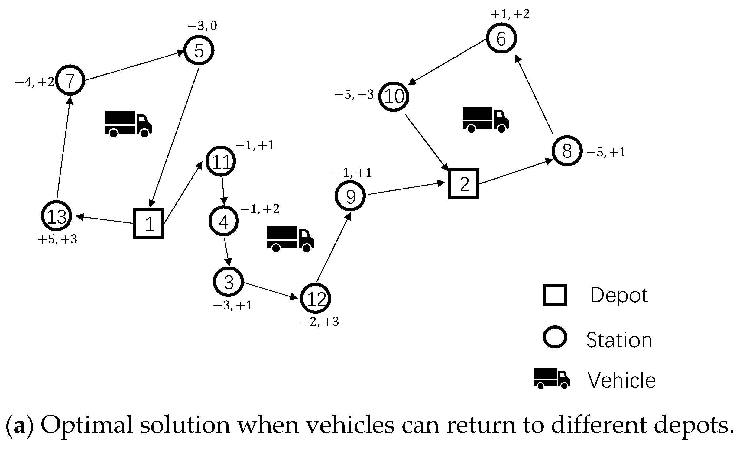
5.4. Comparison Results of Three Strategies

We compare the results of three scenarios in this section. For small instances, we compare three strategies: (1) vehicles can start from and return to different depots; (2) vehicles should start from and return to the same depot; and (3) allowing multiple uses of vehicles. The results are reported in

Table 11. Comparison results for three scenarios.

Instance	${\mathit{n}}_{\mathit{v}\mathit{e}\mathit{h}}$			${\mathit{n}}_{\mathit{v}\mathit{e}\mathit{h}}$			$\mathit{t} \left(\mathit{s}\right)$
	Diff 1	Same 2	Multi 3	Diff	Same	Multi	Diff	Same	Multi
1Bari	16,500	16,500	16,500	2	2	2	0.9	0.6	1.3
2Bari	15,500	16,500	16,500	2	2	2	0.6	0.8	1.1
3Bari	19,400	19,800	18,800	3	3	2	1.8	3.2	8.8
4ReggioEmilia	18,100	18,900	18,900	2	2	2	1.6	8.0	544.7
5ReggioEmilia	17,300	17,300	17,300	2	2	2	1.0	0.9	12.0
6ReggioEmilia	21,800	21,800	21,800	2	2	2	4.1	4.7	14.6
7Bergamo	14,200	14,200	14,200	2	2	2	1.5	1.8	1.6
8Bergamo	14,500	14,500	14,500	2	2	2	11.2	9.6	9.5
9Bergamo	19,200	20,100	19,500	3	3	3	87.0	379.9	73.9
10Parma	31,200	31,500	31,500	2	2	2	0.7	0.7	5.5
11Parma	32,800	32,800	32,800	2	2	2	1.7	1.5	4.9
12Parma	37,400	37,900	37,900	3	3	3	17.1	19.8	52.9
13Treviso	33,546	33,546	33,546	2	2	2	86.1	87.3	239.0
14Treviso	34,423	34,447	34,447	2	2	2	71.4	159.0	73.5
15Treviso	37,495	37,527	36,495	3	4	2	1396.1	1690.7	566.9
Average	24,224.3	24,488.0	24,312.5	2.3	2.3	2.1	112.2	157.9	107.3

¹: vehicles can start from and return to different depots; ²: vehicles should start from and return to same depot; ³: allowing multiple uses of vehicles.

. We can observe that allowing vehicles to return to different depots can obtain better objective values than asking them to return to the same depots for many instances. The number of vehicles used in the first two strategies is always the same, except for instance “15 Treviso”. When vehicles are allowed to use multiple times, the number of vehicles used on average is 2.1, which is smaller than that number for the other two strategies (2.3). Although the benefit of reducing needed vehicles is not very significant for these small-sized instances, we can still observe it in instances “3Bari” and “15Treviso”.

Table 12. Performance of assignment heuristic.

Instance			VNS-DP		VNS-DP + Assignment Heuristic
$\left|\mathit{V}\right|$	$\left|{\mathit{V}}^{\mathit{D}}\right|$	$\mathit{Q}$	Total Time	${\mathit{n}}_{\mathit{v}\mathit{e}\mathit{h}}$	Total Time	%gap	${\mathit{n}}_{\mathit{v}\mathit{e}\mathit{h}}$	%gap	$\mathit{t} \left(\mathit{s}\right)$
150	5	10	37,455.0	26.0	41,125.6	9.8	6.6	−74.6	27.4
150	5	10	43,210.0	28.7	49,580.6	14.7	7.8	−72.8	25.4
150	5	10	43,707.0	25.3	49,320.0	12.8	8.2	−67.8	31.1
150	5	10	37,209.0	25.0	38,356.1	3.1	6.3	−74.8	29.3
150	4	20	35,909.0	18.0	37,054.0	3.2	6.1	−66.0	77.0
150	4	20	35,393.0	15.0	40,269.0	13.8	7.0	−53.3	129.9
150	4	20	32,560.0	20.3	36,485.1	12.1	6.0	−70.4	68.5
200	5	12	41,643.0	30.0	45,776.7	9.9	7.4	−75.3	39.6
200	5	12	40,906.0	28.8	43,915.3	7.4	7.1	−75.3	44.1
200	4	20	46,153.0	20.0	49,302.1	6.8	8.2	−58.9	124.2
200	4	20	47,161.0	18.0	48,756.0	3.4	8.7	−51.9	176.0
249	5	15	67,595.0	30.0	67,213.0	−0.6	10.5	−65.0	76.5
249	5	15	56,193.0	37.3	64,579.8	14.9	10.3	−72.4	41.0
300	5	15	68,302.0	35.0	68,813.5	0.7	11.0	−68.6	120.6
300	5	15	82,097.0	36.9	84,683.0	3.1	13.4	−63.7	72.2
300	5	15	90,349.0	36.0	92,651.7	2.5	15.6	−56.7	74.0
300	5	20	73,752.0	29.0	79,199.3	7.4	13.7	−52.7	144.1
300	6	20	77,660.0	35.0	83,726.5	7.8	14.5	−58.6	81.3
Average			53,180.8	27.5	56,711.5	7.4	9.4	−65.5	76.8

presents the results of the assignment heuristic. We use the assignment heuristic to solutions obtained by VNS-DP to minimize the number of vehicles for large-size instances ($\left|V\right|=150$ to 300). The results of using the assignment heuristic are compared with solutions obtained by VNS-DP. Total time is the average total working time of solutions. We can see that there is a significant reduction in the number of vehicles used. For example, for the first instance, the average number of vehicles required is 26.0 before using a heuristic. This value reduces to 6.6 after using this heuristic, and this induces a 9.8% increase in total working time. The results indicate that the number of required vehicles has a reduction of 65.5% on average compared with the single use of vehicles for large-size instances, and the total working time has an increase of 7.4% on average.

6. Conclusions

This study presents a multi-depot static bike rebalancing and collection problem, which considers multiple depots and broken bike collection. We classify the problem as a two-commodity vehicle routing problem with pickup and delivery and formulate it as an integer programming model. A hybrid solution method, i.e., VNS–DP, which incorporates the restricted DP into the framework of VNS, is developed to solve the problem. The algorithm is equipped with a heuristic for constructing initial solutions, a shaking procedure for exploring different neighborhoods, traditional local search operators, and DP improvement to improve solution quality. The effectiveness of the proposed method is proven by computational experiments on benchmark instances and randomly generated instances. These instances vary in size from 10 to 300 vertices and 2 to 6 depots. The results show that the VNS-DP finds 26 best solutions out of 36 instances, while CPLEX obtains 16 best solutions. We also test the impact of broken bike collection and distribution of depots. The results show that considering broken bike collection increases the transportation cost and reduces the computational time compared with traditional SBRP. More depots provide more choices for vehicles to find better departures and destinations, which leads to a reduction in transportation costs. Comparison of different practical strategies indicates that the number of vehicles can be reduced by 69.4% when allowing multiple visits to depots. Allowing vehicles to return to different depots can help reduce the total working time.

In future work, we should extend the current problem and solution method to consider more flexible situations, such as multiple types of vehicles, multiple visits to stations and multiple service levels. Furthermore, BSS without designated docking stations rapidly increased in recent days and differ from the system investigated in this research. New BRPs should be built to help improve the service quality of such new systems. Incorporating determination of ideal inventory for each station is also a good future direction.