Article

A New Cure Rate Model Based on Flory–Schulz Distribution: Application to the Cancer Data

1
Department of Statistics And Computer Sciences, University of Mohaghegh Ardabili, Ardabil 56199-11367, Iran
2
Departamento de Matematica, Facultad de Ingenieria, Universidad de Atacama, Copiapo 1530000, Chile
3
Departamento de Ciencias Matemáticas y Físicas, Facultad de Ingeniería, Universidad Católica de Temuco, Temuco 4780000, Chile
*
Author to whom correspondence should be addressed.
Mathematics 2022, 10(24), 4643; https://doi.org/10.3390/math10244643
Submission received: 9 November 2022 / Revised: 28 November 2022 / Accepted: 29 November 2022 / Published: 8 December 2022
(This article belongs to the Special Issue Statistical Methods and Models for Survival Data Analysis)

Abstract

:
In this article a new flexible survival cure rate model is introduced by assuming that the number of competing causes of the event of interest follows the Flory–Schulz distribution and the competing causes follow the generalized truncated Nadarajah–Haghighi distribution. Parameter estimation for the proposed model is derived based on the maximum likelihood estimation method. A simulation study is performed to show the performance of the ML estimators. We discuss three real data applications related to real cancer data sets to assess the usefulness of the proposed model compared with some existing cure rate models for the sake of comparison.

1. Introduction

Historically, cancer is a disease with a high mortality rate in human societies. For this reason, it is of interest to correctly identify the possible relationship between cancer and factors that affect it. A useful way to study cancer progression is to monitor patient survival over time. Identifying the effective factors in the long-term survival of cancer patients is one of the important concerns of medical studies. It also makes sense to identify the exact and appropriate models for cancer patients’ lifetime to evaluate the effectiveness of different treatment methods, and patients’ survival time, as well as identify factors affecting patients’ survival. As of recently, with developments in new drugs, medical advancements and improved treatments, patients with certain types of cancer can live as long as people without cancer and show no recurrence of the disease. These patients are said to be cured or long-term survivors. The remaining patients who show a recurrence of the disease are called non-cured or susceptible. Cure rate models have an important role in medical studies and clinical trials and became popular in reliability and survival analysis. In order to introduce the cure rate models, let M be an unobservable random variable of the initial number of competing causes related to the occurrence of an event of interest of an individual in the population.
For the initial number of competing causes M, several discrete distributions were chosen in the literature. To name a few, de Castro et al. [1], Cancho et al. [2], Yiqi et al. [3], Ortega et al. [4] and D’Andrea et al. [5] considered the negative binomial distribution for M. Leão et al. [6] considered zero-modified geometric distribution for M. Gallardo et al. [7] considered Yule–Simon distribution for M. Gallardo et al. [8] considered polylogarithm distribution for M. Gallardo et al. [9] considered the modified power series family of distributions for M. Cancho et al. [10] considered the power series distribution for the number of competing causes M. Balakrishnan et al. [11] considered the weighted Poisson distribution for M. Balakrishnan and Pal [12] considered the Conway–Maxwell–Poisson distribution for M.
In this work, we introduce a new cure rate model based on the Flory–Schulz (F-S) distribution. The motivations to introduce this model are: (1) The F-S has a PGF in a simple and closer form, very useful in this cure rate model context; (2) P ( M = 0 ) = η 2 also has a simple form. This allows one to, among other things, reparametrize the model in terms of the cure rate directly; (3) the F-S distribution has one parameter, being a parsimonious competitor of the traditional promotion time cure rate model proposed in Chen et al. [13]; (4) the advantage of the proposed model is that the F-S distribution is flexible and also there is over-dispersion in the data, which produces a more flexible cure rate model; (5) to the best of our knowledge, the F-S distribution has not yet been proposed in a cure rate model context for the modeling of the number of competing causes. In addition, we also considered the generalized truncated Nadarajah–Haghighi (GeTNH) distribution (Azimi and Esmailian [14]) for the time-to-event of the concurrent causes, a model proposed recently in the literature.
The contents of this article are organized as follows. In Section 2, we formulate the F-S cure rate model based on Flory–Schulz and GeTNH distributions. In Section 3, we obtain the maximum likelihood estimators and asymptotic confidence interval estimations of the parameters of the F-S cure rate models based on the GeTNH distribution. In Section 4, we analyze three real cancer data sets. In Section 5, we perform a simulation study to evaluate the performance of the ML estimators of model parameters. Finally, in Section 6, we provide some conclusions.

2. Modeling

Let R j , j = 1 , , be a sequence of random variables that denotes the time of occurrence of the event of interest (for example, the number of clonogenic tumor cells at the end of treatment that can produce detectable cancer). Assume that, conditional on M, the R j are independent identically distributed with the common survival function S ( t ) . We also assume that R j , j = 1 , , M are independent of M and define R 0 as P ( R 0 = ) = 1 . M = 0 and M 1 determines the cured and susceptible individuals, respectively. The observable time until the event of interest is defined as (Cancho et al. [10])
T = min { R 0 , R 1 , , R M }
Under this setting and according to Tsodikov et al. [15] and Rodrigues et al. [16], the survival function for the population is given by
S p o p ( t ) = G M ( S ( t ) ) ,
where G M ( . ) is the probability generating function (PGF) of M. Let M denote the number of competing cause random variables related to the occurrence of the event of interest. We consider that random variable M has the F S ( η ) (Flory–Schulz distribution with parameter η ) with probability mass function given as (Flory [17])
P ( M = m ) = η 2 m ( 1 η ) m 1 , m = 1 , 2 , , 0 < η < 1 .
According to Gallardo et al. [7] and Gallardo et al. [8], in the cure rate contexts, M is a random variable with support on set { 0 , 1 , 2 , } . Therefore, we shift the probability mass function in (3) to the form of
P ( M = m ) = η 2 ( m + 1 ) ( 1 η ) m , m = 0 , 1 , 2 , , 0 < η < 1 ,
with PGF
G M ( s ) = m = 0 P ( M = m ) s m = η 2 ( 1 + ( η 1 ) s ) 2 , 0 s 1 .
Specifically, applying the F-S model in the discussed previous cure rate models framework and from Equation (2), the survival function for the population is given by
S p o p ( t ) = η 2 ( 1 + ( η 1 ) S ( t ) ) 2 , t 0 .
Hereafter, we refer to the model appearing in Equation (4) as the Flory–Schulz cure rate (F-SCR) model. From Equation (4) and as S ( t ) is a proper survival function, the cure rate immediately is given by
p = lim t + S p o p ( t ) = η 2 .
Thus, the cured fraction is an increasing function of η . Henceforth, we adopt the parameterization p = η 2 , i.e., η = p 1 2 . In this way, covariates can be directly linked to the cure rate p, allowing to compare regression coefficients among different models parameterized in terms of the cure rate.
With the parameterization in the cure rate p, the survival function of the F-SCR model for the population from Equation (4) is given by
S p o p ( t ) = p ( 1 + ( p 1 2 1 ) S ( t ) ) 2 , t 0 .
From Equation (5), the probability density function (PDF) of the population is given by
f p o p ( t ) = d d t S p o p ( t ) = 2 p ( 1 p 1 2 ) f ( t ) 1 + ( p 1 2 1 ) S ( t ) 3 ,
where S ( t ) is the survival function and f ( t ) is the probability density function of the latent event times R 1 , R 2 . Since S p o p ( t ) is not a proper survival function, the f p o p ( t ) is not a proper PDF either. The hazard function associated to PDF Equation (6) is given by
h p o p ( t ) = 2 ( 1 p 1 2 ) f ( t ) 1 + ( p 1 2 1 ) S ( t ) .
Moreover, we note that in the negative binomial (NBCR) cure rate model (Rodrigues et al. [16]) if θ = 1 η 0.5 η and α = 0.5 , the NBCR cure rate model reduces to the F-SCR model. As mentioned, there are some important special cases in the F-SCR model, such as having one parameter and simple form and simply reparametrizing the model in terms of the cure rate. In this context it is very common to use the Weibull distribution as the model for R 1 , R 2 , the time-to-event of the concurrent causes. This is explained because the Weibull model has a simple expression for the survival function and the hazard rate assumes different shapes depending only on its shape parameter. Alternatively, in this work we propose, for the first time in a cure rate model context, the use of the GeTNH distribution because its hazard function can assume increasing, decreasing, bathtub shaped or increasing–decreasing (upside-down bathtub shaped) depending on the parameter values. The PDF for the GeTNH model is
f ( t ) = α β λ t β 1 e t β 1 A 1 + λ e t β α 1 e 1 1 + λ e t β α , t > 0 , α > 0 , λ > 0 , β > 0 ,
where A = e 1 ( 1 + λ ) α . The survival function of GeTNH distribution is given by
S ( t ) = 1 e 1 1 + λ e t β α A 1 A , t > 0 .
For this particular case (considering GeTNH distribution to the time of the event of interest), we refer to the model as the F-SCR/GeTNH model and the PDF, CDF and associated survival functions are given by
f p o p ( t ) = 2 α β ( 1 p ) p λ t β 1 e t β e 1 1 + λ e t β α 1 + λ e t β α 1 1 A 1 + ( p 1 ) 1 e 1 1 + λ e t β α A 1 A 3 ,
S p o p ( t ) = p 1 + ( p 1 ) 1 e 1 1 + λ e t β α A 1 A 2 ,
and
h p o p ( t ) = 2 α β ( 1 p ) λ t β 1 e t β e 1 1 + λ e t β α 1 + λ e t β α 1 1 A 1 + ( p 1 ) 1 e 1 1 + λ e t β α A 1 A ,
respectively.
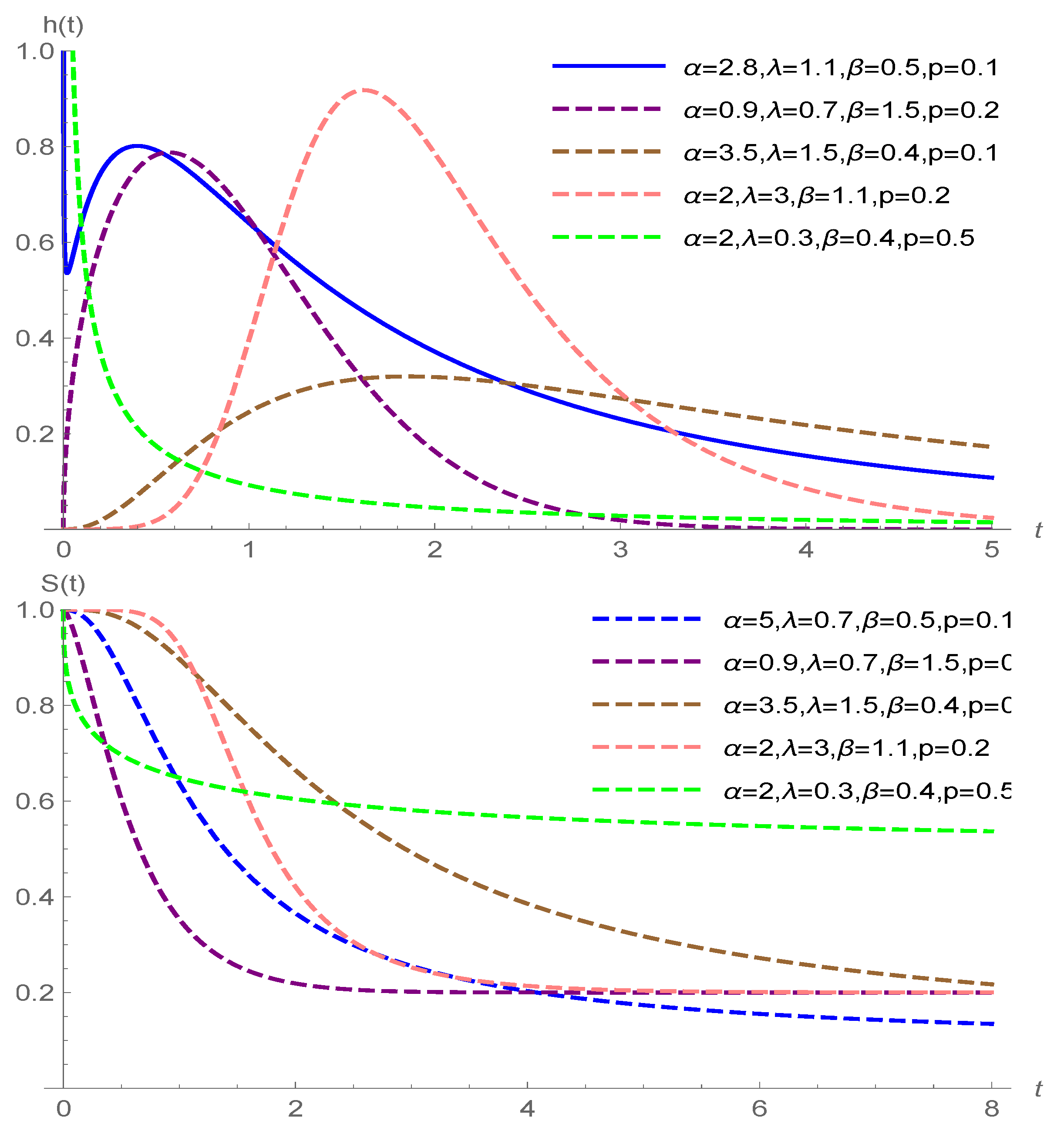
The different shapes of the HRF and survival function of the F-SCR/GeTNH model are illustrated in Figure 1. Note that the HRF of the F-SCR/GeTNH model is very flexible and can be decreasing, bathtub shaped or increasing–decreasing (upside-down bathtub shaped) depending on the parameter values. This wide range of HRF shapes allows more flexibility concerning F-SCR/GeTNH model distribution for analyzing real lifetime data sets in many areas of reliability and survival analysis.

3. Inference

In this section, the parameters for the F-SCR/GeTNH are derived based on the maximum likelihood (ML) method. We consider the lifetimes as subject to right censoring. Let Y i and C i be the failure and censoring time variables for the ith individual, respectively. In a random sample of size n, we observed T i = min ( Y i , C i ) and δ i = I ( Y i C i ) , where δ i = 1 and δ i = 0 denote that a failure or a censoring time was observed for the ith individual, respectively. Additionally, to avoid the identifiability problems discussed in Li et al. [18] and Hanin and Huang [19], we assume that the population is heterogeneous, so we considered a vector of dimension s, say x i = ( 1 , z 1 i , , z s i ) , related to the cure rate. Such covariates can be linked with p i as
log p i 1 p i = γ 0 + γ 1 x 1 i + + γ s x s i
where γ = ( γ 0 , γ 1 , , γ s ) is a vector of unknown regression coefficients. Under those assumptions, these covariates are linked to the parameter p in the following way:
p i = exp ( x i γ ) 1 + exp ( x i γ ) , i = 1 , , n .
The notation ⊤ indicates the transpose. Under the usual assumptions in survival analysis (independence between T i and C i , independence among the observations and non-informative censoring, Williams and Lagakos [20]), the log-likelihood of the model is given by
( Θ ) = i = 1 n δ i log f p o p ( t ) + i = 1 n ( 1 δ i ) log S p o p ( t ) = i = 1 n δ i log 2 α β λ 1 A + ( β 1 ) i = 1 n δ i log t i i = 1 n δ i t i β + ( α 1 ) i = 1 n δ i log ( Z i ) + i = 1 n δ i ( 1 Z i α ) i = 1 n ( δ i + 2 ) log 1 + exp ( x i γ ) 1 + exp ( x i T γ ) 1 1 e 1 Z i α 1 A + i = 1 n δ i log 1 exp ( x i γ ) 1 + exp ( x i γ ) + i = 1 n log exp ( x i γ ) 1 + exp ( x i γ ) ,
where Z i = 1 + λ e t i β , and Θ = ( α , λ , β , γ ) .
The ML estimators of the model are derived by numerical maximization of the log-likelihood function Equation (8). To maximize the log-likelihood function, we used the NMaximize function in the MATHEMATICA 12.0 software.
Further, the confidence intervals of the model parameters with covariates based on the asymptotic distributions of their ML estimators are derived. Under certain regularity conditions presented in Appendix A, Θ ^ = ( α ^ , λ ^ , β ^ , γ ^ ) is approximately distributed as a multivariate normal distribution with mean Θ = ( α , λ , β , γ ) and covariance matrix Σ ( Θ ^ ) , which can be estimated by
Σ ^ ( Θ ^ ) = 2 ( Θ ) Θ Θ Θ = Θ ^ 1 .
The approximate ( 1 ζ ) 100 % confidence intervals of the parameters α , λ , β and the components of γ are
α ^ ± z ζ 2 v a r ^ ( α ^ ) , λ ^ ± z ζ 2 v a r ^ ( λ ^ ) , β ^ ± z ζ 2 v a r ^ ( β ^ ) , γ s ^ ± z ζ 2 v a r ^ ( γ s ^ ) ,
where z ζ 2 is the ζ 2 quantile of the standard normal distribution.

4. Applications: Data Analysis

We provide applications of the F-SCR model to three real cancer data sets. We compare the F-SCR model with the most popular cure rate models, namely, Bernoulli (BeCR) and binomial (BCR) cure rate models (D’Andrea et al. [5]), Poisson (PCR) cure rate model (Chen et al. [13]) and the NBCR based on GeTNH, Nadarajah–Haghighi (NH) and Weibull distributions by considering Akaike’s information criterion (AIC) (Akaike [21]), Bayesian information criterion (BIC) (Schwarz [22]) and Hannan–Quinn information criterion (HQIC) (Hannan and Quinn [23]). These criteria are computed for some models. Lower AIC, BIC and HQIC values indicate a better model. The survival function for these cure rate models parameterized in terms of the cure rate are presented as Appendix B. We also compare the Kaplan–Meier estimator to fitting the data through the survival curves of models. In this section, all calculations were performed using maxLik package of R software [24] with the Newton–Raphson maximization method and NMaximize function in the MATHEMATICA 12.0 software with the Nelder–Mead maximization method.

4.1. Colon Cancer Data

The colon cancer data set relates to the recurrence or death of colon cancer patients. This data set has 1858 observations and 50.58% censoring (938 in total) is availible in the survival package [25] of R [24]. The mean and standard deviation of the observed survival time (measured in years) are 4.2124 and 2.5937, respectively. For more details concerning this data set, see Laurie et al. [26]. For computational purposes, we convert all observations from days to years. For the colon data set, the following covariate variables are available:
  • node4: x i 1 , more than four positive lymph nodes (0 = no, 1 = yes),
  • sex: x i 2 (1 = male, 0 = female),
  • etype: x i 3 (1 = recurrence, 2 = death),
  • surg: x i 4 , time from surgery to registration (0 = short, 1 = long),
  • extent: x i 5 , extent of local spread (1 = submucosa, 2 = muscle, 3 = serosa, 4 = contiguous structures).
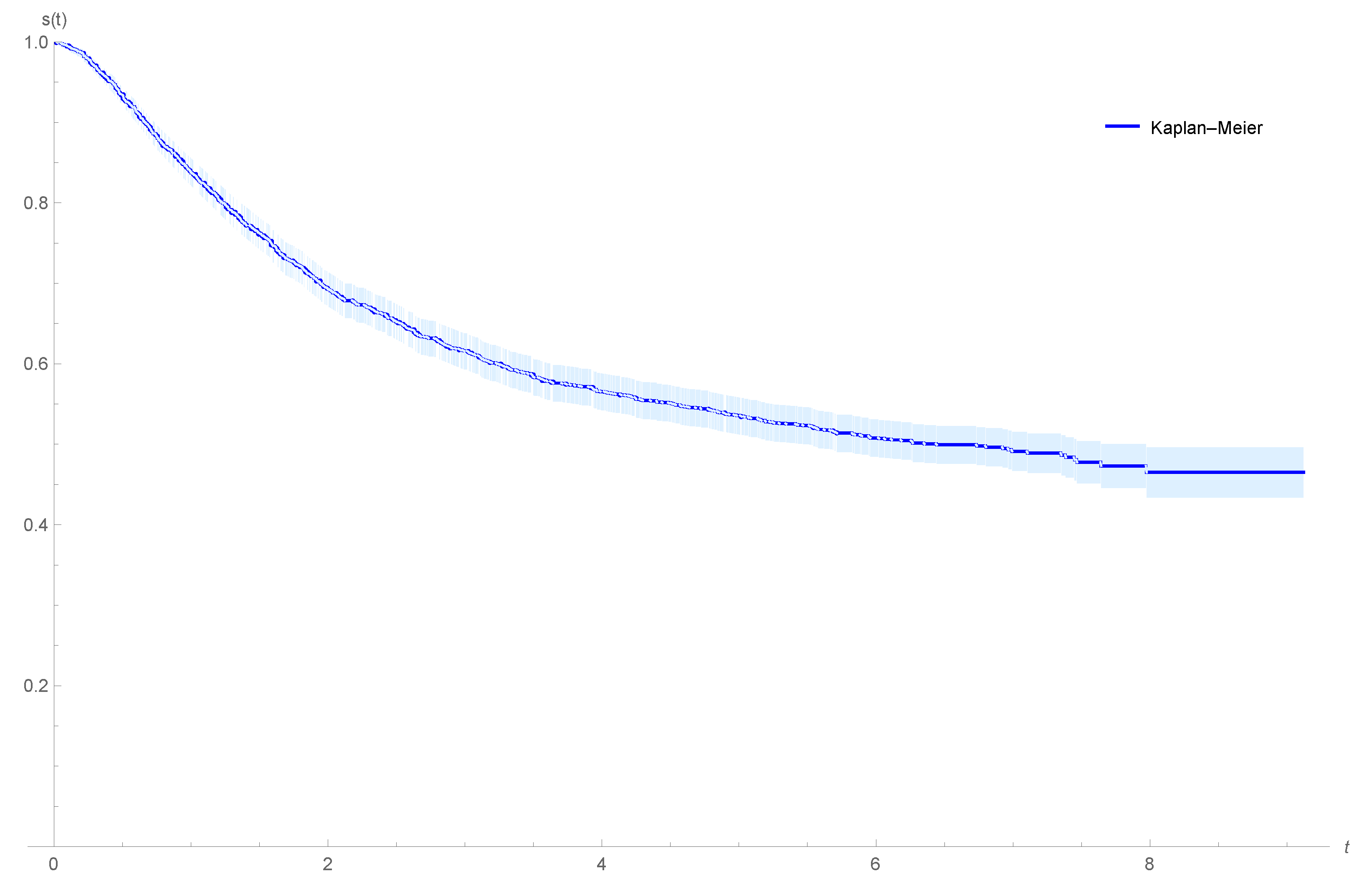
Figure 2 shows the plot of the Kaplan–Meier estimator for the survival function of the colon data. We observe that a proportion of colon cancer for the patients will never recur, and the patients censored at the end of the experiment may be immune, suggesting that the patients can be considered as cured.
Table 1, Table 2 and Table 3 provide the ML estimators of the parameters and corresponding information criteria for the colon cancer data, assuming the GeTNH, NH and Weibull distributions for the time-to-event for the concurrent causes. AIC, BIC and HQIC in Table 1, Table 2 and Table 3 indicate that the F-SCR/GeTNH model has the lowest value, and it is best fit among the BeCR/GeTNH, BCR/GeTNH, PCR/GeTNH, NBCR/GeTNH, F-SCR/NH, BeCR/NH, BCR/NH, PCR/NH, NBCR/NH, F-SCR/We, BeCR/We, BCR/We, PCR/We and NBCR/We cure rate models in terms of fitted information criteria. Therefore, comparing the AIC, BIC and HQIC in Table 1, Table 2 and Table 3, we realize that the F-SCR/GeTNH model provides a better fit to the colon cancer data. In Table 1 and Table 2 the estimated lower bound of the approximate confidence intervals of the parameters α and λ in some cases is negative values. Since α > 0 and λ > 0 , we convert all negative values to zero (0 * ).
From Table 1 and using the F-SCR/GeTNH model, we conclude that the parameters γ 1 n o d e 4 , γ 3 e t y p e , γ 4 s u r g and γ 5 e x t e n t have a significant effect on the cure rate (95% confidence interval for γ 1 n o d e 4 , γ 3 e t y p e , γ 4 s u r g , γ 5 e x t e n t 1 and γ 5 e x t e n t 3 , not including zero) and γ 5 e x t e n t 2 and γ 1 s e x has no significant influence on the cure rate. Figure 3 shows the plots of the estimated survival functions of the F-SCR/GeTNH model for the colon cancer data stratified by sex status for patients with more than four positive lymph nodes (0 = no, 1 = yes); event type: recurrence; time from surgery to registration: short; extent of local spread: serosa.
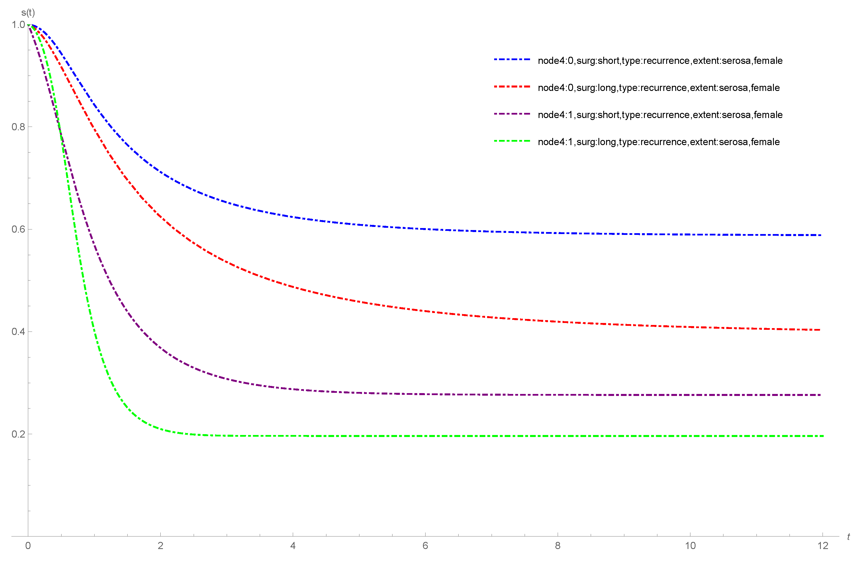
Figure 4 shows the plots of the estimated survival functions of the F-SCR/GeTNH model for the colon cancer data stratified by surg status for patients with more than four positive lymph nodes (0 = no, 1 = yes); event type: recurrence; sex: female; extent of local spread: serosa. From Figure 3 and Figure 4, we observe that the cure rate of the patients with more than four positive lymph nodes (yes) is less than the cure rate of the patients with more than four positive lymph nodes (no). According to Figure 3, in the case of more than four positive lymph nodes (no), the cure rate of the male patients is less than the cure rate of the female patients. In the case of more than four positive lymph nodes (yes) the cure rate of the female patients is less than the cure rate of the male patients. According to Figure 4, in the case of more than four positive lymph nodes (no and yes), the cure rate of the patients with a long time from surgery to registration is less than the cure rate of the patients with a short time from surgery to registration.

4.2. Melanoma Cancer Data

This melanoma cancer data set is related to the phase III cutaneous melanoma clinical trial in which patients were observed for recurrence after the removal of a malignant melanoma described and analyzed by Ibrahim et al. [27]. The data set, labeled E1690, is available at http://merlot.stat.uconn.edu/~mhchen/survbook/ (accessed on 15 October 2022).The original sample has 427 patients (417 observations and 10 missing) with 55.63% censored elements (232 in total); the mean and standard deviation of the observed lifetimes (measured in years) are 3.18 and 1.69, respectively. For the melanoma data set, we considered the following covariate variables:
  • age: x i 1 , classified as zero when the age was below the third quartile (57.56 years) and as one otherwise;
  • nodes1: x i 2 , nodule category 1 to 4, with 4 being the most severe category of cancer;
  • perform: x i 3 , performance status. This means a patient’s functional capacity scale as regards his or her daily activities (0: fully active, 1: other);
  • sex: x i 4 , (0: male; 1: female).
Figure 5 shows the Kaplan–Meier estimator for the survival function of the melanoma cancer data, suggesting that there is a proportion of patients in the population with melanoma cancer that can be considered cured. Table 4 shows the ML estimators of the parameters and corresponding information criteria for the melanoma cancer data, assuming GeTNH for the time-to-event for the concurrent causes. AIC, BIC and HQIC in Table 4 indicate that the F-SCR/GeTNH model has the lowest value, and it is best fit among the BeCR/GeTNH, BCR/GeTNH, PCR/GeTNH and NBCR/GeTNH cure rate models in terms of fitted information criteria. Therefore, comparing AIC, BIC and HQIC in Table 4, we realize that the F-SCR/GeTNH model provides a better fit to the melanoma cancer data. From Table 4 and using the F-SCR/GeTNH model, we conclude that the parameter γ 2 n o d e s 1 has a significant effect on the cure rate (95% confidence interval for γ 2 n o d e s 1 , not including zero) and γ 1 a g e , γ 3 p e r f o r m and γ 4 s e x have no significant influence on the cure rate. 
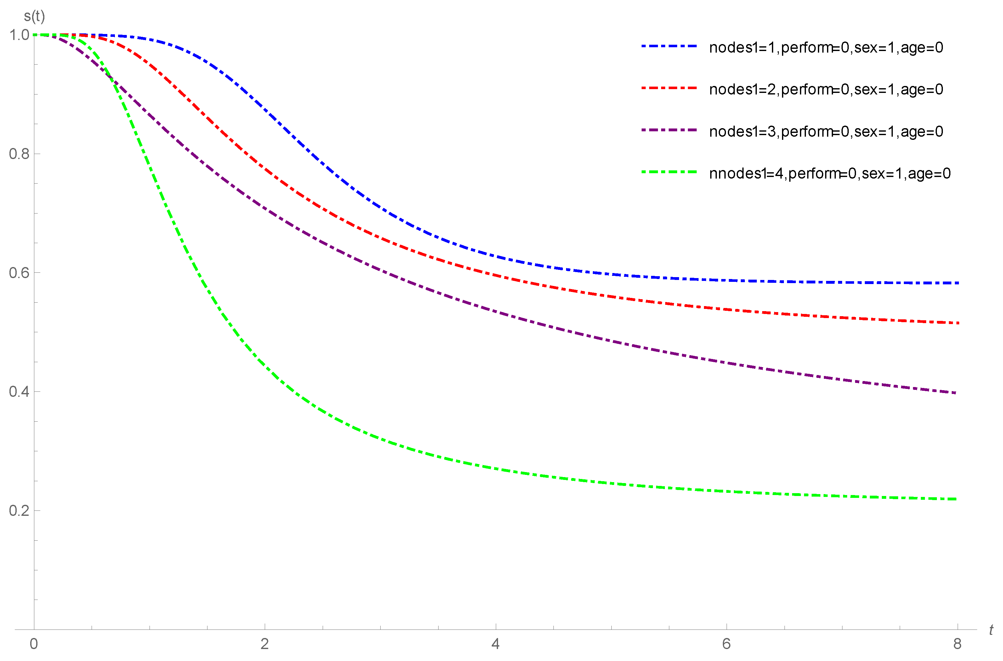
Figure 6 shows the plots of the estimated survival functions of the F-SCR/GeTNH model for the melanoma cancer data stratified by nodule category (1 to 4); perform: fully active; sex: female; age: below 57.56. From Figure 6, we observe that the cure rate of the melanoma cancer patients with nodule category 1 is more than the cure rate of the patients with nodule category 2 to 4.

4.3. Oropharynx Cancer Data

This oropharynx cancer data set is related to the survival time of 195 patients with carcinoma of the oropharynx. For the oropharynx cancer data, the percentage of censored observations is nearly 27.1% (53 in total). For computational purposes, let us consider the survival time from days to years. The mean and standard deviation of the observed survival time (measured in years) are 1.53 and 1.14, respectively. These data are available in Kalbfleisch and Prentice [28]. For the oropharynx data set, the following covariates are associated with each participant:
  • age: x i 1 (0: less than 60 years; 1: greater or equal to 60 years);
  • T stage: x i 2 ; 1: primary tumour measuring 2 cm or less in largest diameter; 2: primary tumour measuring 2 cm to 4 cm in the largest diameter with minimal infiltration in depth; 3: primary tumour measuring more than 4 cm; 4: massive invasive tumour,
  • N stage: x i 3 ; 0: no clinical evidence of node metastases; 1: single positive node 3 cm or less in diameter, not fixed; 2: single positive node more than 3 cm in diameter, not fixed; 3: multiple positive nodes or fixed positive nodes;
  • sex: x i 4 (1: male; 2: female).
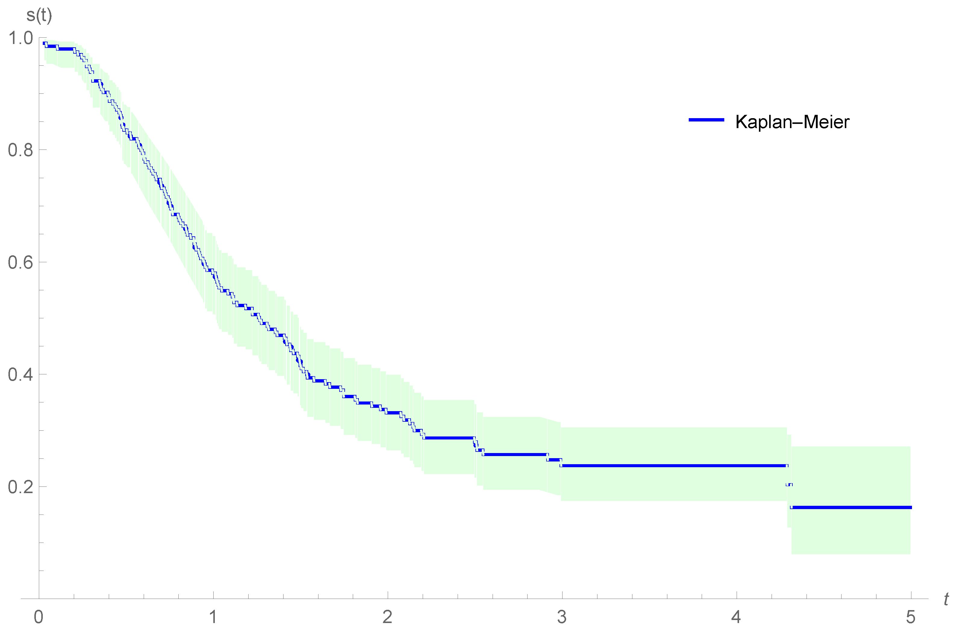
Figure 7 shows the Kaplan–Meier estimator for the survival function of the oropharynx cancer data, suggesting that there is a proportion of patients in the population with oropharynx cancer that can be considered cured. Table 5 shows the ML estimators of the parameters and corresponding information criteria for the oropharynx cancer data, assuming GeTNH for the time-to-event for the concurrent causes. AIC, BIC and HQIC in Table 5 indicate that the F-SCR/GeTNH model has the lowest value, and it is best fit among the BeCR/GeTNH, BCR/GeTNH, PCR/GeTNH and NBCR/GeTNH cure rate models in terms of fitted information criteria. Therefore, comparing the AIC, BIC and HQIC in Table 5, we realize that the F-SCR/GeTNH model provides a better fit to the oropharynx cancer data. From Table 5 and using the F-SCR/GeTNH model, we conclude that the parameters γ 2 T s t a g e and γ 3 N s t a g e have a significant effect on the cure rate (95% confidence interval for γ 2 T s t a g e and γ 3 N s t a g e , not including zero) and γ 1 a g e and γ 4 s e x have no significant influence on the cure rate. 
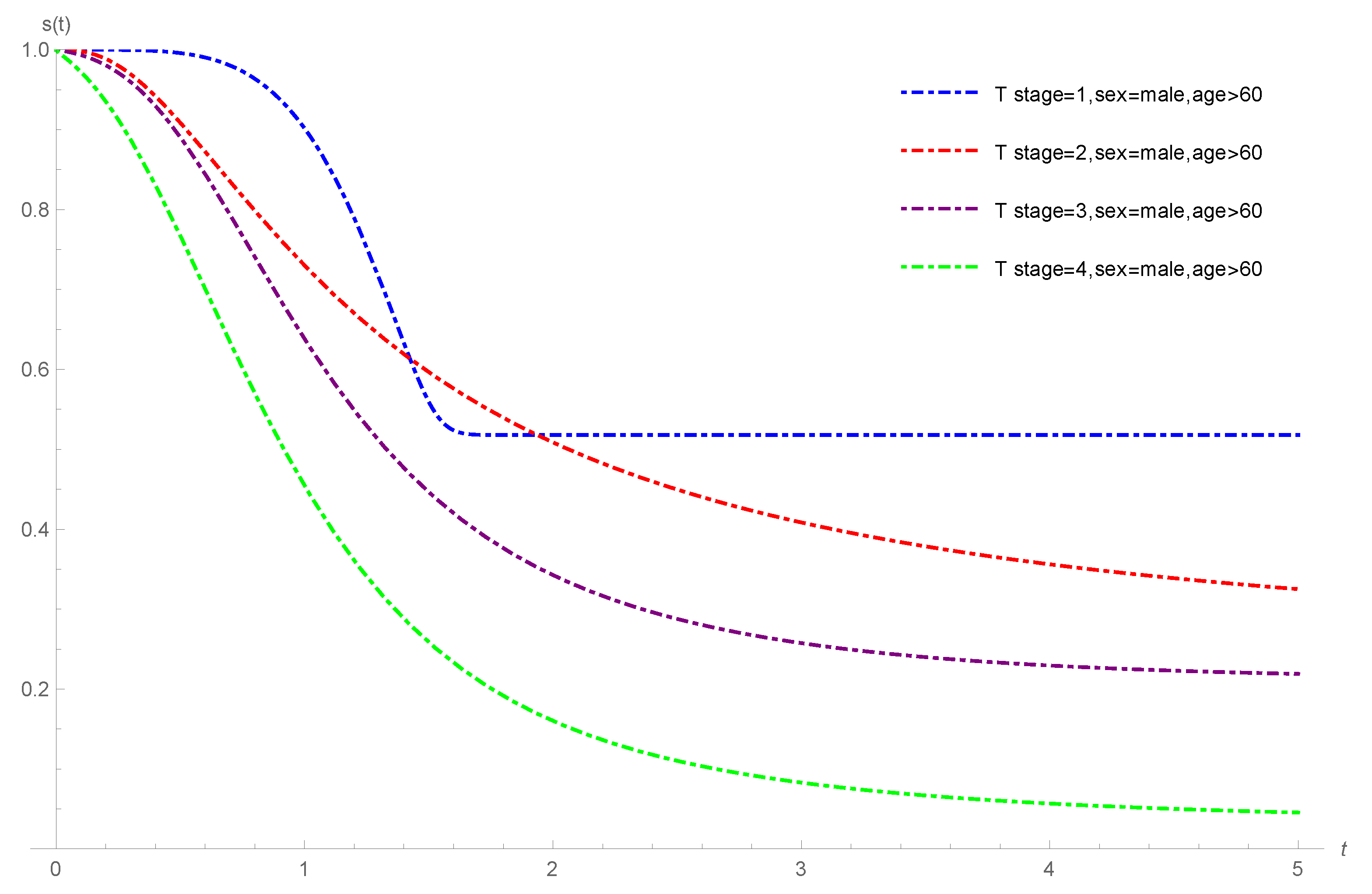
Figure 8 shows the plots of the estimated survival functions of the F-SCR/GeTNH model for the oropharynx cancer data stratified by T stages 1 to 4; sex: male; age: greater than or equal to 60 years. From Figure 8, we observe that the cure rate of the oropharynx cancer patients with T stage 1 is more than the cure rate of the oropharynx cancer patients with T stage 2 to 4.

5. Simulation Study

In this section, we present a simulation study to show the accuracy of the ML estimators of the parameters of the F-SCR model based on GeTNH distribution with covariates. Applying a similar algorithm due to Kutal and Qian [29], the right-censored samples of size n from the F-SCR model based on GeTNH distribution are generated as follows.
Step 1:
Fix the parameter values, α > 0 , λ > 0 and β > 0 , as well as the value of the cure fraction 0 < p < 1 .
Step 2:
Generate n random samples from u i U ( 0 , 1 )
Step 3:
The random survival time can be calculated from the equation
t i = F 1 ( U i ) = log 1 log 1 ( 1 A ) p 1 U i 1 ( p 1 ) 1 1 α 1 λ 1 β ,
if u i 1 p ; otherwise, t i is infinity.
Step 4:
Generate the simple sample of the censoring times c 1 , , c n from a GeTNH distribution and adjust the parameters of the GeTNH distribution to obtain the desired censoring rates.
Step 5:
Calculate y i = min ( t i , c i ) . Pairs of simulated values ( y i , δ i ) , i = 1 , , n are thus obtained, where δ i = 1 if y i c i and δ i = 0 if y i > c i . In the simulation study, we pick the F-SCR model with three covariates x 1 , x 2 and x 3 , where x 1 B e r n o u l l i ( 0.5 ) , x 2 U ( 0 , 2 ) and x 2 U ( 0 , 2 ) . In the case of high cure rate the initial values of parameters are ( α , λ , β ) = ( 1.3 , 0.75 , 0.45 ) and in the case of low cure rate they are ( α , λ , β ) = ( 0.6 , 0.4 , 0.45 ) . The initial value of γ 0 , γ 1 , γ 2 and γ 3 is computed from four combinations of values of ( x 1 , x 2 , x 3 ) and cure rates p 1 , p 2 , p 3 , p 4 . For ( x 1 , x 2 , x 3 ) , we choose (0, 0, 0), (1, 0, 0), (0, 1, 2) and (1, 2, 1). In the studies, we also consider two levels of the cure rate, say high cure rate (0.8, 0.7, 0.6, 0.5) and low cure rate (0.25, 0.2, 0.15, 0.10). Solving the four equations resulting from Equation (7), for high cure rate we obtain γ 0 = 1.3862 , γ 1 = 0.5389 , γ 2 = 0.2379 and γ 3 = 0.3714 , and for low cure rate we obtain γ 0 = 1.0981 , γ 1 = 0.2876 , γ 2 = 0.1536 and γ 3 = 0.3286 .
For the simulations, we take the sample sizes n = 400 , 600 , 800 , 1000 . We replicate the simulations 1000 times and evaluate the estimated bias of ML estimators and the mean square errors (MSEs). The program codes are available once requested. Based on simulation results in Table 6 we observe that the MSEs for ML estimators decrease when the sample size n increases. In fact, the ML estimators tend to be closer to the true parameter values when the sample size n increases, suggesting that the ML estimators for the F-SCR/GeTHN are consistent in finite samples.

6. Conclusions

In this work, we proposed a new cure rate model for survival data assuming several competing causes of the event of interest follow the F-S distribution. For the time of the event of interest, we proposed a GeTNH distribution that is more flexible than other lifetime models to estimate the cure rate fraction and effects of the covariates on cure rate fraction. The MLE method was applied to estimate the parameters of the F-SCR/GeTHN model. The performance of the ML estimators was confirmed by the simulation study. In the empirical applications related to colon cancer data, oropharynx cancer data and melanoma cancer data, we discovered that the F-SCR/GeTHN model provided the best fit among other common models proposed in the literature. Therefore, the F-S distribution can be an appropriate alternative discrete distribution for modeling of the number of competing causes of the event of interest in comparison with the common models proposed in the literature. Further research in this line should involve a scheme based on random effects or error-in-variable for the F-Scr model. Moreover, generalizations of the F-S distribution can result in a more flexible distribution that could be appropriated for modeling of the number of competing causes of the event of interest. Work in this direction is currently under progress and we hope to report these findings in a future paper.

Author Contributions

Conceptualization: R.A. and M.E.; Formal analysis: R.A. and M.E.; Investigation: R.A. and H.J.G.; Software: R.A. and D.I.G.; Supervision: M.E. and D.I.G.; Writing—Review editing: D.I.G. and H.J.G. All of the authors contributed significantly to this research article. All authors have read and agreed to the published version of the manuscript.

Funding

This research received no external funding.

Data Availability Statement

The data used in Section 4 is duly referenced.

Acknowledgments

The authors would like to thank the editors and the anonymous reviewers for their constructive comments, which led to improving the quality of the manuscript.

Conflicts of Interest

The authors declare no conflict of interest.

Appendix A. Regularity Conditions

If f ( x ; θ ) denotes the density of the underlying random variables, the MLE score function is
U n ( x , θ ) = θ l o g f ( x ; θ ) .
Under the Cramér–Rao-Fréchet regularity conditions (see Sen et al. [30], page 47, Theorem 2.3.1) and the uniform continuity condition (see Sen et al. [30], page 245, Equation 8.3.2), the solution to the estimating equations with the above score function is a n -consistent estimator θ ^ n of θ such that
n ( θ ^ n θ ) D N ( 0 , [ I f ( θ ) ] 1 ) ,
where I f ( θ ) is the per unit observation Fisher information matrix on θ .

Appendix B. The Survival Function for Cure Rate Models Parameterized in Terms of the Cure Rate

  • BeCR/GeTNH survival function (D’Andrea et al. [5])
    S p o p ( t ) = p + ( 1 p ) S ( t ) = p + ( 1 p ) 1 e 1 1 + λ e t β α 1 A ,
  • BCR/GeTNH survival function (D’Andrea et al. [5]) ( n = 3 )
    S p o p ( t ) = p 1 3 + ( 1 p 1 3 ) S ( t ) 3 = p 1 3 + ( 1 p 1 3 ) 1 e 1 1 + λ e t β α 1 A 3 ,
  • NBCR/GeTNH survival function ( θ = 0.3 ) (Rodrigues et al. [16])
    S p o p ( t ) = 1 + ( p 0.3 1 ) ( 1 S ( t ) ) 1 0.3 = 1 + ( p 0.3 1 ) 1 1 e 1 1 + λ e t β α 1 A 1 0.3 ,
  • PCR/GeTNH survival function (Chen et al. [13])
    S p o p ( t ) = p 1 S ( t ) = p 1 1 e 1 1 + λ e t β α 1 A .

References

  1. De Castro, M.; Gomez, Y.M. A Bayesian Cure Rate Model Based on the Power Piecewise Exponential Distribution. Methodol. Comput. Appl. Probab. 2020, 22, 677–692. [Google Scholar] [CrossRef]
  2. Cancho, V.G.; Rodrigues, J.; de Castro, M. A flexible model for survival data with a cure rate: A Bayesian approach. J. Appl. Stat. 2011, 38, 57–70. [Google Scholar] [CrossRef]
  3. Yiqi, B.; Russo, C.M.; Cancho, V.G.; Louzada, F. Influence diagnostics for the Weibull-Negative-Binomial regression model with cure rate under latent failure causes. J. Appl. Stat. 2015, 43, 1027–1060. [Google Scholar] [CrossRef]
  4. Ortega, E.M.M.; Cordeiro, G.M.; Kattan, M.W. The negative binomial–beta Weibull regression model to predict the cure of prostate cancer. J. Appl. Stat. 2012, 39, 1191–1210. [Google Scholar] [CrossRef]
  5. D’Andrea, A.; Rocha, R.; Tomazella, V.; Louzada, F. Negative Binomial Kumaraswamy-G Cure Rate Regression Model. J. Risk Financ. Manag. 2018, 11, 6. [Google Scholar] [CrossRef] [Green Version]
  6. Leão, J.; Bourguignon, M.; Gallardo, D.I.; Rocha, R.; Tomazella, V. A new cure rate model with flexible competing causes with applications to melanoma and transplantation data. Stat. Med. 2020, 39, 1–13. [Google Scholar] [CrossRef]
  7. Gallardo, D.I.; Gómez, H.W.; Bolfarine, H. A new cure rate model based on the Yule-Simon distribution with application to a melanoma data set. J. Appl. Stat. 2017, 44, 1153–1164. [Google Scholar] [CrossRef]
  8. Gallardo, D.I.; Gómez, Y.M.; Castro, M.D. A flexible cure rate model based on the polylogarithm distribution. J. Stat. Comput. Simul. 2018, 88, 2137–2149. [Google Scholar] [CrossRef]
  9. Gallardo, D.I.; Gómez, Y.M.; Gómez, H.W.; de Castro, M. On the use of the modified power series family of distributions in a cure rate model context. Stat. Methods Med. Res. 2019, 29, 1831–1845. [Google Scholar] [CrossRef]
  10. Cancho, V.G.; Louzada-Neto, F.; Ortega, E.M.M. Ortega. The Power Series Cure Rate Model: An Application to a Cutaneous Melanoma Data. Commun.-Stat.-Simul. Comput. 2013, 42, 586–602. [Google Scholar] [CrossRef]
  11. Balakrishnan, N.; Koutras, M.V.; Milienos, F. A weighted Poisson distribution and its application to cure rate models. Commun.-Stat.-Theory Methods 2018, 47, 4297–4310. [Google Scholar] [CrossRef]
  12. Balakrishnan, N.; Pal, S. Expectation maximization-based likelihood inference for flexible cure rate models with Weibull lifetimes. Stat. Methods Med. Res. 2016, 25, 1535–1563. [Google Scholar] [CrossRef] [PubMed]
  13. Chen, M.H.; Ibrahim, J.G.; Sinha, D. A New Bayesian Model for Survival Data with a Surviving Fraction. J. Am. Stat. Assoc. 1999, 94, 909–919. [Google Scholar] [CrossRef]
  14. Azimi, R.; Esmailian, M. A New Generalization of Nadarajah–Haghighi Distribution with Application to Cancer and COVID-19 Deaths Data. Math. Slovaca 2022. (accepted). [Google Scholar]
  15. Tsodikov, A.D.; Ibrahim, J.G.; Yakovlev, A.Y. Estimating Cure Rates from Survival Data: An Alternative to Two-Component Mixture Models. J. Am. Stat. Assoc. 2003, 98, 1063–1078. [Google Scholar] [CrossRef] [PubMed] [Green Version]
  16. Rodrigues, J.; Cancho, V.G.; de Castro, M.; Louzada-Neto, F. On the Unification of the Long-term Survival Models. Stat. Probab. Lett. 2009, 79, 753–759. [Google Scholar] [CrossRef]
  17. Flory, P.J. Molecular Size Distribution in Linear Condensation Polymers. J. Am. Chem. Soc. 1936, 58, 1877–1885. [Google Scholar] [CrossRef]
  18. Li, C.S.; Taylor, J.M.; Sy, J.P. Identifiability of cure models. Stat. Probab. Lett. 2001, 54, 389–395. [Google Scholar] [CrossRef]
  19. Hanin, L.; Huang, L. Identifiability of cure models revisited. J. Multivar. Anal. 2014, 130, 261–274. [Google Scholar] [CrossRef]
  20. Williams, J.S.; Lagakos, S.W. Models for Censored Survival Analysis: Constant-Sum and Variable-Sum Models. Biometrika 1997, 64, 215–224. [Google Scholar]
  21. Akaike, H. A new look at the statistical model identification. IEEE Trans. Autom. Control. 1974, 19, 716–723. [Google Scholar] [CrossRef]
  22. Schwarz, G.E. Estimating the dimension of a model. Ann. Stat. 1978, 6, 461–464. [Google Scholar] [CrossRef]
  23. Hannan, E.J.; Quinn, B.G. The Determination of the order of an autoregression. J. R. Stat. Soc. Ser. B 1979, 41, 190–195. [Google Scholar] [CrossRef]
  24. R Core Team R: A Language and Environment for Statistical Computing; R Foundation for Statistical Computing: Vienna, Austria, 2014; Available online: http://www.R-project.org/ (accessed on 1 November 2022).
  25. Therneau, T.M.; A Package for Survival Analysis in R. R Package Version 3.2-13. 2021. Available online: https://CRAN.R-project.org/package=survival (accessed on 1 November 2022).
  26. Laurie, J.A.; Moertel, C.G.; Fleming, T.R.; Wieand, H.S.; Leigh, J.E.; Rubin, J.; McCormack, G.W.; Gerstner, J.B.; Krook, J.E.; Malliard, J. Surgical adjuvant therapy of large-bowel carcinoma: An evaluation of levamisole and the combination of levamisole and fluorouracil. the north central cancer treatment group and the Mayo. J. Clin. Oncol. Off. J. Am. Soc. Clin. Oncol. 1989, 7, 1447–1456. [Google Scholar] [CrossRef]
  27. Ibrahim, J.G.; Chen, M.H.; Sinha, D. Bayesian semiparametric models for survival data with a cure fraction. Biometrics 2001, 57, 383–388. [Google Scholar] [CrossRef]
  28. Kalbfleisch, J.D.; Prentice, R.L. The Statistical Analysis of Failure Time Data; John Wiley & Sons: Hoboken, NJ, USA, 2011; Volume 360. [Google Scholar]
  29. Kutal, D.H.; Qian, L. A Non-Mixture Cure Model for Right-Censored Data with Fréchet Distribution. Stats 2018, 1, 176–188. [Google Scholar] [CrossRef]
  30. Sen, P.K.; Singer, J.M.; Pedroso-de-Lima, A.C. From Finite Sample to Asymptotic Methods in Statistics; Cambridge University Press: New York, NY, USA, 2010. [Google Scholar]
Figure 1. The HRF (first panel) and survival function (second panel) of F-SCR/GeTNH model for different parameter values.
Mathematics 10 04643 g001
Figure 2. Kaplan–Meier curve for the colon data.
Mathematics 10 04643 g002
Figure 3. Plots of the survival functions for the colon data based on F-SCR/GeTNH model stratified by sex status for patients with more than 4 positive lymph nodes (0 = no, 1 = yes); event type: recurrence; time from surgery to registration: short; extent of local spread: serosa.
Mathematics 10 04643 g003
Figure 4. Plots of the survival functions for the colon data based on F-SCR/GeTNH model stratified by surg status for patients with more than 4 positive lymph nodes (0 = no, 1 = yes); event type: recurrence; sex: female; extent of local spread: serosa.
Mathematics 10 04643 g004
Figure 5. Kaplan–Meier curve for the melanoma data.
Mathematics 10 04643 g005
Figure 6. Plots of the survival functions for the melanoma data based on F-SCR/GeTNH model stratified by nodule category (1 to 4); perform: fully active; sex: female; age: below 57.56.
Mathematics 10 04643 g006
Figure 7. Kaplan–Meier curve for the oropharynx data.
Mathematics 10 04643 g007
Figure 8. Plots of the survival functions for the oropharynx cancer data based on F-SCR/GeTNH model stratified by T stage (1 to 4); sex: male; age: greater than or equal to 60 years.
Mathematics 10 04643 g008
Table 1. ML estimators (95% confidence intervals) and information criteria for the colon cancer data set based on GeTNH distribution.
ParameterF-SCRBeCRPCRBCR (n = 3)NBCR  ( θ = 0.3 )
α 4.3951 (0.6745, 8.1158)254916 (0 * , 61.6073)8.3250 (1.8283, 14.8216)11.8014 (4.2472, 19.3556)5.5195 (0 * , 11.2536)
λ 0.7715 (0.0477, 1.4953)0.0898 (0 * , 0.2192)0.3467 (0.0614, 0.6321)0.2240 (0.0750, 0.3729)0.5748 (0 * , 1.2229)
β 0.4607 (0.3577, 0.5643)0.5872 (0.5220, 0.6535)0.4845 (0.4060, 0.5629)0.5179 (0.4476, 0.5882)0.4679 (0.3671, 0.5688)
γ 0 i n t e r c e p t −1.7108 (−2.3432, −1.0783)−1.0427 (−1.8952, −0.1901)−1.5487 (−2.2566, −0.8408)−1.3594 (−2.1085, −0.6104)−1.6609 (−2.3275, −0.9944)
γ 1 n o d e 4 −1.4150 (−1.6399, −1.1900)−1.5918 (−1.9791, −1.2045)−1.5324 (−1.8078, −1.2570)−1.5733 (−1.8830, −1.2636)−1.4652 (−1.7089, −1.2215)
γ 2 s e x 0.0234 (−0.1680, 0.2148)−0.0494 (−0.2795, 0.1805)0.0044 (−0.2044, 0.2134)−0.0136 (−0.2312, 0.2039)0.0161 (−0.1825, 0.2149)
γ 3 e t y p e 0.4773 (0.2853, 0.6693)0.1442 (−0.0848, 0.3733)0.3816 (0.1725, 0.5908)0.3030 (0.0856, 0.5203)0.4436 (0.2444, 0.6428)
γ 4 s u r g −0.3559 (−0.6270, −0.0847)−0.5282 (−0.8868, −0.1704)−0.4197 (−0.7248, −0.1147)−0.4568 (−0.7830, −0.1323)−0.3813 (−0.6659, −0.0966)
γ 5 e x t e n t 1 1.9283 (1.0315, 2.8253)2.0967 (1.0200, 3.1734)2.0359 (1.0741, 2.9978)2.0438 (1.0475, 3.0401)1.9774 (1.0546, 2.9001)
γ 5 e x t e n t 2 −0.3559 (−0.9082, 0.1964)1.7761 (0.9681, 2.5841)1.7596 (1.1200, 2.3992)1.7698 (1.0779, 2.4617)1.7146 (1.1280, 2.3012)
γ 5 e x t e n t 3 1.9283 (1.4568, 2.3999)0.9470 (0.2103, 1.6837)0.9172 (0.3552, 1.4791)0.9171 (0.3007, 1.5335)0.8881 (0.3810, 1.3952)
AIC5273.425342.465293.825309.275281.06
BIC5334.225403.265354.625370.075341.86
HQIC5295.835364.865316.225331.685303.47
F-SCR: Flory–Schulz cure rate model, BeCR: Bernoulli cure rate model, BCR: binomial cure rate model, PCR: Poisson cure rate model, NBCR: negative binomial cure rate model.
Table 2. ML estimators (95% confidence intervals) and information criteria for the colon cancer data set based on NH distribution.
ParameterF-SCRBeCRPCRBCR (n = 3)NBCR  ( θ = 0.3 )
α 8.0827 (0 * , 40.8266)1.3739 (0.8832, 1.8647)3.3845 (0.4263, 6.3427)2.1514 (0.9370, 3.3658)1.3408 (0 * , 2.8064)
λ 0.0241 (0 * , 0.1234)0.2609 (0.1497, 0.3722)0.0702 (0.0055, 0.1349)0.1275 (0.0487, 0.2062)0.1547 (0.0105, 0.2990)
γ 0 i n t e r c e p t −1.2567 (−1.8094, −0.7041)−0.7394 (−1.4285, −0.0503)−1.1281 (−1.7334, −0.5228)−1.0044 (−1.6390, −0.3699)0.0590 (−0.5741, 0.6922)
γ 1 n o d e 4 −1.3012 (−1.5103, −1.0921)−1.3790 (−1.6593, −1.0986)−1.3887 (−1.6206, −1.1568)−1.4059 (−1.6533, −1.1586)−1.3500 (−1.5930, −1.1076)
γ 2 s e x 0.0180 (−0.1658, 0.2018 )−0.0399 (−0.2496, 0.1697)0.0016 (−0.1931, 0.1964)−0.0155 (−0.2122, 0.1891)0.0102 (−0.1822, 0.2027)
γ 3 e t y p e 0.4169 (0.2329, 0.6009)0.1324 (−0.0764, 0.3414)0.3406 (0.1460, 0.5351)0.2722 (0.0720, 0.4724)0.2969 (0.1046, 0.4892)
γ 4 s u r g −0.3422 (−0.5262, −0.1581)−0.4609 (−0.7752, −0.1466)−0.3888 (−0.6694, −0.1083)−0.4161 (−0.7089, −0.1232)−0.5492 (−0.8309, −0.2675)
γ 5 e x t e n t 1 1.8593 (0.9833, 2.7354)1.8636 (0.9021, 2.8250)1.8709 (0.9649, 2.7768)1.8763 (0.9505, 2.8021)0.3137 (−0.5514, 1.1788)
γ 5 e x t e n t 2 1.5598 (1.0356, 2.0841)1.5378 (0.8796, 2.1959)1.6046 (1.0276, 2.1816)1.5947 (0.9897, 2.1998)0.1146 (−0.4464, 0.6758)
γ 5 e x t e n t 3 0.7879 (0.3430, 1.2328)0.7667 (0.1790, 1.3544)0.8143 (0.3111, 1.3175)0.8054 (0.2724, 1.3385)−0.5144 (−1.0106, −0.0182)
AIC5351.465400.355360.525372.075397.35
BIC5406.735455.635415.795427.345452.62
HQIC5371.835420.725380.895392.445417.22
F-SCR: Flory–Schulz cure rate model, BeCR: Bernoulli cure rate model, BCR: binomial cure rate model, PCR: Poisson cure rate model, NBCR: negative binomial cure rate model.
Table 3. ML estimators (95% confidence intervals) and information criteria for the colon cancer data set based on Weibull distribution.
ParameterF-SCRBeCRPCRBCR (n = 3)NBCR  ( θ = 0.3 )
α 1.3870 (1.3033, 1.4706)1.2638 (1.1873, 1.3404)1.3110 (1.2315, 1.3905)1.2678 (1.1906, 1.3451)1.3552 (1.2733, 1.4371)
λ 3.4296 (3.0848, 3.7743)2.4872 (2.3097, 2.6647)3.0634 (2.7882, 3.3386)2.8324 (2.5963, 3.0685)3.2821 (2.9663, 3.5980)
γ 0 i n t e r c e p t −1.3696 (−1.9265, −0.8130)0.4224 (−0.1586, 1.0036)−1.1840 (−1.7891, −0.5789)−1.0136 (−1.6389, −0.3883)−1.3097 (−1.8882, −0.7311)
γ 1 n o d e 4 −1.3721 (−1.9289, −0.8154)−1.2403 (−1.4862, −0.9944)−1.4100 (−1.6414, −1.1786)−1.4032 (−1.6448, −1.1617)−1.3944 (−1.6147, −1.1741)
γ 2 s e x 0.0236 (−0.1884, 0.2358)−0.0894 (−0.2908, 0.1119)0.0052 (−0.1894, 0.2000)−0.0089 (−0.2082, 0.1903)0.0169 (−0.1725, 0.2064)
γ 3 e t y p e 0.4622 (0.2769, 0.6476)0.1135 (−0.0868, 0.3139)0.3592 (0.1646, 0.5539)0.2802 (0.0814, 0.4790)0.4246 (0.2350, 0.6143)
γ 4 s u r g −0.3460 (−0.6077, −0.0843)−0.1777 (−0.4685, 0.1130)−0.3880 (−0.6684, −0.1077)−0.4112 (−0.7013, −0.1211)−0.3637 (−0.6334, −0.0940)
γ 5 e x t e n t 1 1.8766 (1.0021, 2.7511)−0.3295 (−1.1358, 0.4766)1.9038 (0.9965, 2.8110)1.8838 (0.9623, 2.8053)1.8976 (1.0087, 2.7866)
γ 5 e x t e n t 2 1.6349 (1.1025, 2.1674)0.4546 (−0.1042, 1.0136)1.6456 (1.0660, 2.2252)1.6076 (1.0074, 2.2079)1.6509 (1.0975, 2.2042)
γ 5 e x t e n t 3 0.8398 (0.3858, 1.2938)−0.4032 (−0.8844, 0.0778)0.8491 (0.3427, 1.3555)0.8191 (0.2903, 1.3479)0.8531 (0.3757, 1.3304)
AIC5289.165414.955315.325335.085298.92
BIC5344.435470.225370.595390.355354.19
HQIC5309.535435.325335.695355.455319.29
F-SCR: Flory–Schulz cure rate model, BeCR: Bernoulli cure rate model, BCR: binomial cure rate model, PCR: Poisson cure rate model, NBCR: negative binomial cure rate model.
Table 4. ML estimators (95% confidence intervals) and information criteria for the melanoma cancer data set based on GeTNH distribution.
ParameterF-SCRBeCRPCRBCR (n = 3)NBCR  ( θ = 0.01 )
α 2.7341 (0 * , 6.7091)11.8753 (0 * , 33.3400)3.7032 (0 * , 10.5647)4.813 (0 * , 15.0957)3.706 (0 * , 7.4403)
λ 1.3627 (0 * , 3.7506)0.2138 (0 * , 0.6180)0.8785 (0 * , 2.7420)0.62 (0 * , 2.0907)0.8774 (0 * , 1.8854)
β 0.6855 (0.4123, 0.9587)0.7691 (0.6189, 0.9193)0.7085 (0.4566, 0.9603)0.7276 (0.5039, 0.9512)0.7087 (0.5103, 0.9070)
γ 0 i n t e r c e p t 0.8855 (0.0811, 1.6899)0.9445 (0.0160, 1.8731)0.9269 (0.1007, 1.7530)0.9456 (0.1106, 1.7805)0.9356 (0.1031, 1.7680)
γ 1 a g e −0.1819 (−0.5895, 0.2111)−0.2928 (−0.7564, 0.1706)−0.2287 (−0.6546, 0.1972)−0.2535 (−0.6933, 0.1863)−0.229 (−0.6558, 0.1978)
γ 2 n o d e s 1 −0.5181 (−0.7080, −0.3283)−0.5023 (−0.7312, −0.2734)−0.5270 (−0.7318, −0.3221)−0.5427 (−0.7557, −0.3296)−0.5277 (−0.7329, −0.3224)
γ 3 p e r f o r m −0.2377 (−0.8353, 0.3599)−0.1915 (−0.8935, −0.5105)−0.2412 (−0.8854, 0.4030)−0.2323 (−0.9000, 0.4354)−0.2405 (−0.8810, 0.4000)
γ 4 s e x 0.2313 (−0.1871, 0.6498)0.2416 (−0.2601, 0.7524)0.2457 (−0.1951, 0.6865)0.2487 (−0.2042, 0.7016)0.2466 (−0.1891, 0.6823)
AIC1031.991040.921034.461036.451035.90
BIC1064.251073.191066.721068.711068.17
HQIC1044.741053.681047.211049.211048.66
F-SCR: Flory–Schulz cure rate model, BeCR: Bernoulli cure rate model, BCR: binomial cure rate model, PCR: Poisson cure rate model, NBCR: negative binomial cure rate model.
Table 5. ML estimators (95% confidence intervals) and information criteria for the oropharynx cancer data set based on GeTNH distribution.
ParameterF-SCRBeCRPCRBCR (n = 3)NBCR  ( θ = 0.01 )
α 2.8366 (0 * , 5.9192)92.1391 (82.3222, 101.9559)7.8794 (0 * , 17.7203)69.1816 (51.0566, 87.3065)9.3282 (0 * , 18.8265)
λ 1.0798 (0 * , 2.5329)0.0156 (0.0120, 0.0191)0.2585 (0 * , 0.6475)0.0276 (0.0189, 0.0362)0.2405 (0 * , 0.5015)
β 0.7931 (0.4626, 1.1235)1.1181 (0.9013, 1.3348)0.8437 (0.5528, 1.1345)0.9086 (0.64106, 1.1761)0.8402 (0.5512, 1.1291)
γ 0 i n t e r c e p t 0.5378 (−1.2467, 2.3223)0.5604 (−1.9027, 3.0235)0.6971 (−1.3454, 2.7396)0.729 (−1.5204, 2.9784)0.6657 (−1.4416, 2.7730)
γ 1 a g e 0.1405 (−0.4627, 0.7437)0.1198 (−0.7535, 0.9931)0.1401 (−0.5776, 0.8578)0.1293 (−0.6633, 0.9219)0.1354 (−0.5807, 0.8515)
γ 2 T s t a g e −0.627 (−1.0150, −0.2389)−0.615 (−1.1624, −0.0675)−0.6796 (−1.1413, −0.2178)−0.6904 (−1.2021, −0.1786)−0.6674 (−1.1329, −0.2019)
γ 3 N s t a g e −0.294 (−0.5495, −0.0384)−0.2668 (−0.6454, 0.1118)−0.3114 (−0.6212, −0.0015)−0.311 (−0.6581, 0.0361)−0.3071 (−0.6257, 0.0115)
γ 4 s e x 0.2054 (−0.4931, 0.9039)0.2395 (−0.7212, 1.2002)0.2455 (−0.5669, 1.0579)0.2661 (−0.6190, 1.1512)0.2453 (−0.5845, 1.0751)
AIC463.49475.45466.15468.37465.86
BIC489.67501.63492.33494.55492.04
HQIC474.09486.05476.75478.97476.46
F-SCR: Flory–Schulz cure rate model, BeCR: Bernoulli cure rate model, BCR: binomial cure rate model, PCR: Poisson cure rate model, NBCR: negative binomial cure rate model.
Table 6. Simulated bias of the ML estimators of the parameters and their corresponding MSE in the simulation studies with covariates.
Levels of the Cure RateHigh Cure RateLow Cure Rate
n ParametersBiasMSEBiasMSE
400 α −0.15190.8403−0.30380.8452
λ −0.40090.3222−0.15070.1749
β −0.0290.00250.05420.0007
γ 0 −1.25071.6593−0.09720.1422
γ 1 −0.50830.32480.10130.1063
γ 2 0.18760.05810.06900.0337
γ 3 0.37950.16290.29390.1121
600 α −0.15320.6861−0.36270.2544
λ −0.4660.3219−0.16640.1583
β −0.02690.00190.05310.0006
γ 0 −1.19431.529−0.12030.1246
γ 1 0.49930.31030.13500.0887
γ 2 0.21180.05080.08110.0301
γ 3 0.35920.13770.28740.1037
800 α −0.19720.6233−0.37060.2499
λ −0.47480.3276−0.14220.1482
β −0.02550.00170.05160.0004
γ 0 −1.19591.5223−0.10930.1217
γ 1 0.50700.30370.12670.0856
γ 2 0.20890.04880.07730.0275
γ 3 0.36150.13730.28580.1003
1000 α −0.18960.5862−0.41170.2341
λ −0.47990.3260−0.12520.1651
β −0.02610.00160.05180.0004
γ 0 −1.18981.5023−0.12920.1204
γ 1 0.50400.29560.12810.0810
γ 2 0.20810.04810.08070.0253
γ 3 0.35980.13540.28530.0978
Publisher’s Note: MDPI stays neutral with regard to jurisdictional claims in published maps and institutional affiliations.

