Abstract
The Saudi economy ought to maintain a significant amount of foreign exchange reserves due to the pegged exchange rate regime. As a hydrocarbon economy, we measure the dynamic response of external assets and liabilities of banks to the international oil price in Saudi Arabia. In the presence of extreme observations, we apply sophisticated frameworks, including cross-quantilograms, quantile-on-quantile and TVP-VAR approaches, to analyze weekly time-series data from 1993 to 2021. Our results from the cross-quantilogram and quantile-on-quantile frameworks demonstrate that foreign assets and liabilities responded asymmetrically to the volatilities of international oil prices under the bullish and bearish states of the market over different memories. The TVP-VAR results indicate that, during the COVID-19 pandemic, the Saudi economy encountered negative net foreign assets, which occurred mainly as a significant plague of international oil prices. Our findings are robust under different estimators.
MSC:
37M10
1. Introduction
Over the recent decade, the Saudi Arabian economy enjoyed a stable oil revenue along with stable economic growth. The steady oil revenue and economic growth can be attributed to the pegged foreign exchange rate system since June 1986. More importantly, the pegged exchange rate system provided a credible anchor of stability, reduced transaction costs, and simplified the conduct of the macroeconomic policy. Meanwhile, despite some progress in diversification, the Saudi economy remains dependent, to varying degrees, on the hydrocarbon economy and related activities. Despite the stability in the exchange rate, one of the drawbacks of a pegged exchanges rate is that the Saudi Central Bank (SAMA) ought to maintain a significant amount of foreign exchange reserves. Therefore, we are motivated to measure the response of external assets and liability to the international oil price.
The prior literature overwhelmingly stressed the influence of oil prices on the current account and trade balance, which can be classified into two main strands. The first strand of the literature focuses on measuring the impact of the oil price shock on the trade balance (excluding net service export). Several studies investigate the asymmetric effects of oil price on trade balance by decomposing oil and nonoil-derived trade [1,2,3,4,5,6,7]. In contrast, a list of studies measured the impact of oil prices on the overall trade balance [8,9,10,11,12]. For example, Baek [9] investigated the oil price and trade balance nexus in the context of Korea and 14 trading partners by applying an asymmetric approach. The results of Baek [9] demonstrate that the Korean bilateral trade balance fluctuations are associated with oil price volatility. A decrease in oil price elevates export as it reduces production costs, causing an improvement in the trade balance. Interestingly, a rise in the oil price helped the Korean trade balance with Japan and the US, as the economy mostly trades technological products, which are less oil-oriented. Yildirim and Arifli [13] documented that an increase in oil price decreased the trade deficit in Azerbaijan as a narrow base hydrocarbon economy.
The study of Fratzscher et al. [10] is in line with the findings of Backus and Crucini [8], and showed that the oil price shock increased the external liabilities of oil importers. In contrast, the oil supply shock led to a deficit in the trade balance of oil importers, although only after one year, after the shock trade balance was restored [3]. Nasir et al. [12] stressed the response to oil price shocks in BRICS countries by applying a time-varying structural vector autoregressive (TV-SVA) approach. The study found that the impact of oil prices is more profound for Russia than for Brazil, since Russia is a more prominent oil exporter. The balance of trade for Brazil experiences deterioration when the oil price increases. Interestingly, Russia experiences improvements in the trade balance in response to the oil price rising. Among oil-importing countries, India is more sensitive than BRICS member countries to oil price shocks in terms of negative oil price impacts on inflation, GDP, and trade balance. Though oil price shock effects are almost negligible for China, Nasir et al. [12] argued that their influence is more profound. China is an energy-dependent country; thus, maintaining a stable local currency and economic growth puts pressure on the economy.
Ample studies measured the impact of the oil price shock on the overall trade balance, decomposing oil and nonoil flows. For example, Jibril et al. [3] assessed the response of oil, nonoil and overall trade balance to demand and supply shocks of oil prices. The study highlights that oil supply shocks reduce the oil trade balance and the overall trade balance of oil exporter countries, but insignificantly affect the nonoil trade balance. On the contrary, an increase in aggregate demand and oil-specific demand improves the oil balance and overall balance. Hathroubi and Aloui [14] investigated the cyclicality of fiscal policy through the connectedness between oil prices and different macroeconomic indicators in Saudi Arabia. The study found a strong connection between oil prices and several macroeconomic variables. In particular, oil price negatively influences nonoil GDP, but positively impacts government expenditures and the trade balance of Saudi Arabia. Lopez-Murphy and Villafuerte [6] and Bova et al. [2] found similar results that oil-producing countries often follow procyclical fiscal policies due to oil price shocks. More specifically, during 2003–2008, oil-producing countries experienced a crowding-out effect due to increased oil prices and expansionary government expenditures. Oil demand and supply shocks jointly explain approximately half of the net foreign assets where their contribution to oil importers’ current accounts is slightly less than exporter countries [4]. Rafiq et al. [7] explored the influence of oil supply and demand shock on the external balances of oil exporters and importers, including the oil and nonoil trade balances. For the oil-exporting group of countries, a rise in oil prices led to an increase in the oil trade balance and a reduction in oil-exporting countries’ nonoil and total trade balances. Bodenstein et al. [1] and Le and Chang [5] argue that oil price shocks insignificantly explain the trade balance of many economies that oil and nonoil responses offset each other; hence, the overall balance of payment remains unchanged.
The second strand measures the response of the current account (including the net service export) to oil price [15,16,17,18,19,20,21,22,23,24]. Balli et al. [16] and Özlale and Pekkurnaz [22] showed that the oil demand shock has a more noticeable impact on the trade balance than the oil supply shock for Russia and China. For example, the oil supply shock negatively influences the current Chinese account but positively impacts the existing Russian account. As for the oil, demand shock hurts the Chinese trade balance and positively impacts the Russian trade balance. Allegret et al. [15] also focused on demand and supply-side shocks, and revealed that supply-side shocks are more profound than demand-side shocks for both oil importers and exporters. Allegret et al. [15] argued that the effect of demand-driven shock is smoothed through trade channels when oil prices go up due to higher economic activity. Moreover, a higher responsiveness to supply-side shocks indicates a higher energy dependency. Huntington [20] discovered that net oil exporters have a surplus in the current account as a response to oil price shocks. Net oil importers are not affected by oil price shocks, though the trade balance of rich countries can run into a deficit. Huntington [20] argues that oil exporters and wealthier oil importers may observe oil income gains and losses as temporary income sources influencing their savings patterns. By analyzing the influence of oil supply and oil demand shocks, Gnimassoun et al. [18] highlighted that oil demand shocks have a postponed but significantly favorable influence on the current account of Canada, while oil supply shocks are insignificant. Gnimassoun et al. [18] argue that oil demand shocks have a more pronounced impact, because positive oil demand shocks induce a 10% increase in oil prices, while negative oil supply shocks are followed by a slight reduction in oil production of 1%. In addition, a higher oil price intensity (for example, due to the Iraq War in 2002–2003) contributes to the current account in a greater magnitude. Gomes et al. [19] explored the relationship between prices on biofuels and the current account of emerging and developing oil-importing countries exporting agricultural commodities used in biofuel production. The study found that biofuel prices did affect the current account until oil prices reached a particular level. Gomes et al. [19] argue that when the price of oil is above the threshold, the current account of countries, which are biofuel exporters and oil importers at the same time, reduces, because they spend more money on purchasing oil. Oil price fluctuations were shown to negatively impact the Turkish current account with a more pronounced effect in the short term [22]. Varlik and Berument [24] and Özlale and Pekkurnaz [22] documented that oil price shocks increased the current account deficit of Turkey in the short term. Nevertheless, the detrimental effect of oil price shocks disappears in the long run. By decomposing the current account into subcomponents, Varlik and Berument [24] found that the current account was balanced by a surplus or deficit in goods under merchanting, agricultural production, maintenance and repair services, travel, construction, financial services, and compensation of employees. Given the limited number of studies focusing on the response of foreign assets and liability to oil price shocks, we intended to conduct this study in the case of Saudi Arabia, where the economy adopted a pegged exchange rate.
We contribute to the existing literature in several ways. Given the best knowledge, our study is a pioneer in investigating the response of foreign assets and liability to international oil prices under a pegged exchange rate system in Saudi Arabia. We cover the nonlinear extreme quantile dependency among foreign assets, foreign liability, and global oil prices considering weekly, monthly, quarterly, and yearly memories. Our method also considers bidirectional conditional dependency following double-condition quantile distribution. This study’s empirical investigation clearly shows that foreign assets and foreign liability respond positively to international oil prices, mostly in long memory at a moderate quantile of foreign assets, liability, and oil prices (1-year lag). The frequency connectedness analysis shows that the Saudi Arabian economy encounters a downfall in foreign assets due to the plunge in the international oil prices during the early wave of the COVID-19 pandemic.
2. Methodology
2.1. Data, Definition, and Source
We utilized weekly data for the period of January 1993–June 2021. We employed foreign assets (FAs) and foreign liabilities (FLs) as the dependent variables and oil price as our independent variable. The description of variables is represented in Table 1.

Table 1.
Description of variables.
Figure 1 demonstrates the trend of foreign assets, liabilities, and oil price shocks. The graph clearly indicates that oil price was highly volatile. Moreover, the foreign asset was more stable compared to foreign liability.
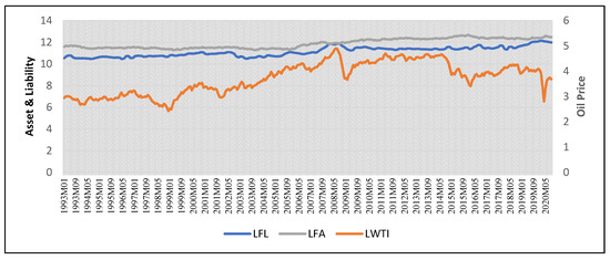
Figure 1.
Trend of foreign asset, liability, and oil price.
2.2. Quantile-on-Quantile Approach
We developed our model as follows:
where is the dependent variable and indicates either foreign liability (FL), foreign asset (FA), or net assets (NAs), and OP is the international oil price.
The quantile-on-quantile (QQ) approach was proposed by Sim and Zhou [11]. This approach has a number of advantages distinguishing this approach from others, such as the typical linear regression or quantile regression. First, the typical linear regression considers the quantiles of the independent variable quantile, whereas quantile regression considers only the quantile of the dependent variable. Meanwhile, the QQ approach combines the aforementioned frameworks and overcomes their limitations by assessing the dynamic influence of each independent variable quantile on each dependent variable quantile under nonparametric properties. Second, compared with the OLS, the QQ framework allows for the detection and capture of the asymmetric response of both the regressand and regressor. Third, the QQ approach overcomes the problem of reverse causality. Specifically, by keeping the quantile of the independent variable fixed, the method estimates its impact on each quantile of the dependent variable. Analogically, the method estimates the influence of each quantile of the independent variable on the quantile of the dependent variable when the latter remains fixed. Thus, the method provides a matrix of slope coefficients. Fourth, since our data were abnormal, we presumed the QQ approach to be the most appropriate method, because it allowed for the presence of outliers, skewness, and kurtosis. These advantages motivated us to employ the QQ approach. We provided the following equation, representing the
-quantile of as a function of oil price:
was not determined, since the relationship between F and OP was not revealed yet. represents the error term with zero meaning quartile. Further, we rewrote Equation (2) into a linear one by employing the first-order Taylor expansion of around as follows:
Afterwards, we rewrote + as functions of and , or . Hence, the latter Equation (3) could be modified as follows:
Finally, by substituting Equation (4) into the initial Equation (3), we obtained the following equation:
2.3. Cross-Quantilogram Dependence
In order to assess the effect of oil price on foreign assets, foreign liabilities, and net assets, we applied the cross-quantilogram (CQ) approach developed by [25], for several reasons. First of all, the method was applicable to different parts of data distribution, including extreme observations as well as the central part of the distribution. Secondly, by using this method, we could calculate the magnitude and duration of the oil price shock’s impact on the dependent variables. Thirdly, the CQ technique employs quantile matches that do not require moment conditions. Hence, the method is suitable for fat-tailed distributions. Finally, the method allowed us to take long lags assessing the strength of the oil price effect, its duration, and direction at the same time.
Equation (6) represents the cross-quantilogram between the two events and , where k signifies the lag length () for a pair of and :
where represents the stationary time series, i is equal to 1, 2, or 3, and indicates the liability, asset, or net asset, and t is time (t = 1, 2,…T). (⋅) and (⋅) are the distribution and density functions of , i = 1, 2. is the corresponding quantile function for , and is the quantile-hit process.
The CQ approach allowed us to find the serial dependence between variables at various quantiles. Moreover, monotonic transformation was considered in both series. In the case of the two events and , means no cross-sectional dependence from event to event . When assessing how varied with the lag length k, we were able to identify how the cross-quantile dependence between foreign liabilities, assets, and net assets varied across different time horizons, thereby quantifying the magnitude and duration of dependence. We considered k = ….. in our study.
Afterwards, we tested the statistical significance of by employing a Ljung–Box-type test, where the t-statistics were calculated as follows (7):
where represents the cross-quantilogram calculated as follows:
where indicates the estimated quantile function.
By applying a stationary bootstrap, we approximated the null distribution of the cross-quantilograms (8) and the Q-statistic (7).
Further, we calculated the partial cross-quantilograms (PCQs) between the OP and dependent variables (FA, FL, and NA) in order to account for the effect of uncertainties. = [] is a vector for of the control variables. The correlation matrix of the quantile hit process and its inverse matrix were defined as:
where is an vector of the quantile hit process. For , let and be the il-th element of and . Note that the cross-quantilogram was . The partial cross-quantilogram was represented as follows:
can be regarded as the cross-quantilogram between and , conditional on the control variable z.
2.4. TVP-VAR
Afterwards, we employed dynamic connectedness under the time-varying parameter vector autoregression (TVP-VAR) approach, developed by Antonakakis and Gabauer [26]. The main advantage of this approach is that it allows for the variance to be different by employing the stochastic volatility Kalman filter estimation and forgetting factors by Koop and Korobilis [27,28]. Hence, the framework allows for overcoming inconsistent parameters that can occur because of the random selection of rolling window size [29]. Moreover, the dynamic connectedness under the TVP-VAR framework was applicable for less frequent data [16], as well as for the short period of time series.
The TVP-VAR estimation was defined as follows:
where denotes the conditional volatility vector and indicates the lagged conditional vector of with dimension. represents the time-varying coefficient matrix following the order. denotes the vector of error with the order along with time-varying covariance matrix . The vector of the coefficient matrix relies on their respective values following the dimensional residual matrix, along with the variance–covariance matrix. This approach subsequently measured the generalized connectedness following [30], considering time-varying parameters and error covariance. This framework eventually allowed us to obtain an estimate of the volatility spillover by utilizing generalized impulse response functions (GIRFs) and generalized forecast error variance decompositions (GFEVDs), as suggested by [28,31]. Thus, by transforming the VAR to the vector moving average (VMA), we obtained representation for GIRF and GFEVD estimation following the Wold theorem, which was defined as:
where and ; consequently, are dimensional parameter matrices following the order .
The GIRFs demonstrated how all respective variables responded to a shock in variable .
We tested the differences between the both when variable was shocked and not shocked, since the model we employed did not follow structural modelling.
Equation (16) shows how we estimated the difference to the shock in variable .
In our study, the oil price was taken as variable , and foreign liabilities, foreign assets, and net assets represented variable , which also reflected the forecasting period, was the selection vector, and represented the information set until . Thereafter, the GFEVD was examined, which was the ratio of variance’s share of one variable to other variables. We normalized the examined variances by merging the rows into one row, representing the forecast error variance of variable being described by all variables. Equation (19) demonstrates the described estimation:
With and By employing the GFEVD, we examined the total connectedness index with the following equations:
The first step of the TVP-VAR was to assess how shock in a variable spillover affected other variables. The process when the shock variable influenced other variables was described as Equation (22):
The second step was to compute the total directional connectedness from others, which showed what spillover effect received from variables j. The calculation was represented as follows:
Eventually, the total directional connectedness to others was subtracted from the total directional connectedness to others. Thus, we obtained the net total directional connectedness, which measured the magnitude of variable impact on the network of variables. The calculation of the net total directional connectedness is shown in Equation (24):
In cases when was positive, the strength of variable impact was more profound than the influence of other variables on variable , indicating that all other variables were influenced with variable . In the contrary, when was negative, the influence of the variable of other variables on variable was more profound than the influence of variable on all other variables.
3. Results and Discussion
3.1. Descriptive Analysis
We started our analysis with descriptive statistics of the return series of each variable (. Table 2 reports that our respective variables followed a non-normal distribution with considerable fluctuations. Moreover, we applied the Elliott–Rothenberg–Stock unit root test. Table 2 confirms that all our variables were stationary at the level. Given the nonabnormality and stationarity, the pre-conditions of the quantile and time-frequency connectedness analysis were satisfied.
Table 2.
Descriptive statistics.
3.2. Cross-Quantilogram
In order to conduct the cross-quantilogram analysis, we considered 19 quantiles with long high-frequency data. We employed 1, 4, 21, and 52 lags, which implied weekly, monthly, semiannual, and yearly data. Figure 2 and Figure 3 represent the results of the cross-quantile dependence from oil price to foreign assets and foreign liabilities, respectively. The results were demonstrated in the form of a heatmap matrix, where black squares indicate a strong dependency, while white squares signify a weak dependency. In addition, the significant relationship was marked with a star sign (where a white star stands for a 10% level of significance and a black star indicates a 5% level of significance).
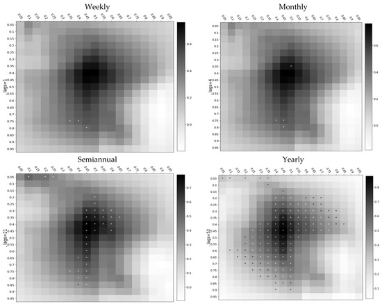
Figure 2.
Cross-quantile dependence from oil price to foreign assets. Note: * indicates significance at 10% level.
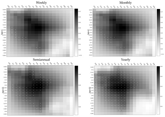
Figure 3.
Cross-quantile dependence from oil price to foreign liabilities. Note: * indicates significance at 10% level.
Figure 2 demonstrates the volatility spillover from oil prices to foreign assets. The weekly heatmap matrix reported that the relationship between the oil price and foreign assets was less significant under weekly memory. Precisely, foreign assets responded positively to oil price shocks under 0.3, 0.35, and 0.4 quantiles of oil price and 0.5 quantiles of foreign assets. We also observed that foreign assets reacted positively to oil price shocks under 0.75 and 0.8 quantiles of oil price and 0.4 and 0.45 quantiles of foreign assets. The intensity of the response of foreign assets substantially increased when we considered them semiannually (21 weeks). Lastly, we incorporated yearly (52 weeks) memory into our analysis. The results demonstrated that the foreign assets responded positively to oil price, with high significance at the middle quantiles of both variables.
Figure 3 highlights the response of foreign liabilities to the international oil price under a four-lag order. Foreign liability responded positively to international oil price volatilities under short memories. Interestingly, the response of liability to oil price was symmetric over weekly and monthly memories. Particularly, oil price under the middle and higher quantiles (0.4–0.85) influenced foreign liabilities under the lower and middle quantiles (0.1–0.5) when considering shorter memory (weekly and monthly). When considering semiannual memory, we observed that the oil price under 0.1–0.9 quantiles influenced foreign liabilities positively under 0.1–0.65 quantiles. Notably, the response of foreign liabilities intensified in the long term.
3.3. Quantile-on-Quantile
By applying the Quantile-on-Quantile approach, we examined the impact of oil price fluctuations on the foreign assets and liabilities of Saudi Arabia by following Chandrarin et al. [32]. We considered nine quantiles in our analysis. Figure 4 and Figure 5 demonstrate the response of foreign assets to oil price fluctuations for monthly and quarterly data, respectively. Figure 4 shows an increase in foreign assets under the quantiles of 0.3, 0.4, and 0.6 as a response to oil price increases in all quantiles (0.1–0.9). The oil price increased under the lower quantiles (0.1 and 0.2), leading to an increase in foreign assets at lower quantiles (0.1, 0.2, and 0.3). However, an increase in oil prices under the quantiles of 0.1–0.9 was associated with a decrease in foreign assets under the medium to higher quantiles. An increase in oil price in the lowest quantile (0.1) was associated with a decrease in foreign assets under the quantile of 0.6. Moreover, an increase in oil price under the quantiles of 0.6, 0.7, 0.8, and 0.9 led to a decrease in foreign assets under the quantiles of 0.1 and 0.2. We argued that oil price shocks mostly led to a decrease in foreign assets because of the higher-frequency data and low-lag structure, indicating that foreign assets could not rapidly adjust to oil price shocks. On the contrary, the results for quarterly data (Figure 5) demonstrated more plots with a positive shock in oil prices and the response of foreign assets, demonstrating that foreign assets required a longer time to adjust. Moreover, foreign assets in the quantiles of 0.8 and 0.9 decreased as a response to an increase in oil price in all quantiles (0.1–0.9), and foreign assets in the lower quantiles (0.1, 0.2) experienced a decrease as a response to an increase in oil price in the higher quantiles of 0.4–0.9. The oil price increase under all quantiles (0.1–0.9) led to an increase in foreign assets under the quantiles of 0.3, 0.4, 0.5, 0.6, and 0.7. An increase in oil price under the quantiles of 0.1, 0.2, and 0.3 resulted in an increase in foreign assets under the quantiles of 0.1 and 0.2. We observed that the foreign assets of Saudi Arabia responded positively to oil price shocks in most quantiles, proving the concept that oil-exporting countries benefit from oil price increases.
Figure 4.
Response of foreign assets to oil price. Monthly data.
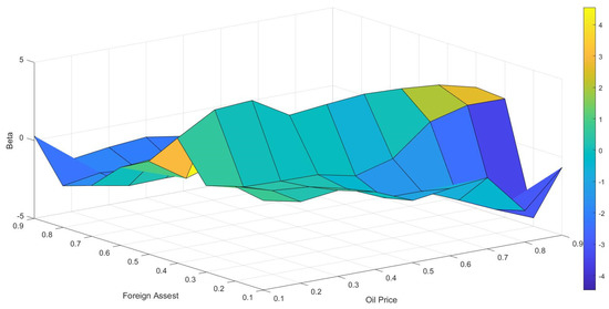
Figure 5.
Response of foreign asset to oil price. Quarterly data.
Figure 6 and Figure 7 highlight the response of foreign liabilities to the oil price. Foreign liabilities plunged under quantiles of 0.6, 0.7, 0.8, and 0.9 as a response to oil price increases under all quantiles (0.1–0.9). Figure 6 depicts foreign liabilities decreasing under the lowest quantiles (0.1 and 0.2) due to oil price shocks under 0.1 quantiles. An increase in oil price under quantiles of 0.2, 0.3, 0.4, 0.5, 0.6, 0.7, 0.8, and 0.9 led to an increase in foreign liabilities under quantiles of 0.1 and 0.2. Foreign liability increased under the quantiles of 0.3, 0.4, and 0.5 as a response to an increase in oil price under all quantiles (0.1–0.9). Thus, higher quantiles of oil price increases resulted in a decrease in foreign liabilities under lower quantiles, meaning that higher oil price was beneficial for Saudi Arabia as an oil-exporting country. Figure 7 shows that Saudi Arabia experienced an increase in foreign liabilities under the quantiles of 0.1, 0.2, 0.3, and 0.4 as a response to oil price in all quantiles (0.1–0.9), except for the 0.2 quantile of foreign liabilities and 0.1 and 0.2 quantiles of oil price. In the higher quantiles (0.5, 0.6, 0.7, 0.8, and 0.9), we observed a decrease in foreign liabilities due to oil price (0.1–0.9 quantiles). When oil price went up, Saudi Arabia experienced an increase in foreign liabilities at lower quantiles and a decrease in foreign liabilities at higher quantiles. This result could be explained by the fact that oil-exporting countries experience an appreciation for local currency with an increase in oil prices, thus, benefiting importing industries. Since Saudi Arabia follows a pegged exchange rate, oil price shocks reflect on foreign liabilities and foreign assets. However, being the most significant net oil exporter in the world, Saudi Arabia gains in a greater magnitude if the price of oil rises, meaning that its foreign liabilities eventually significantly decrease.
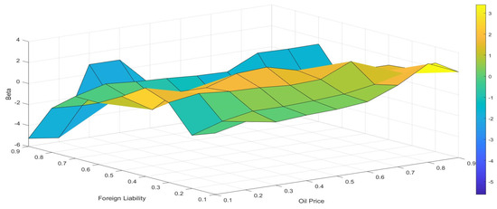
Figure 6.
Response of foreign liabilities to oil price. Monthly data.
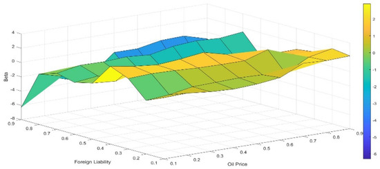
Figure 7.
Response of foreign liability to oil price. Quarterly data.
As for the quarterly data, under the lower quantiles (0.1–0.4), our results demonstrated a deficit in the trade balance (liabilities grew, while assets decreased), whereas under the upper quantiles (0.5–0.9), we could observe a surplus in trade balance (assets grew, while liabilities decreased). As for monthly data, under the higher quantiles (0.6–0.9), we observed the simultaneous growth of assets and liabilities and a simultaneous increase in middle quantiles. Moreover, we observed a trade balance deficit at lower quantiles. The results obtained using the QQ approach were slightly inconsistent with the results of the cross-quantilogram, mainly due to the lag order selection.
This result indicated that oil price fluctuations had a long-term effect on foreign liabilities and assets, consistent with our following results using the quantile-on-quantile approach.
3.4. Time-Frequency Analysis
Oil price mainly acted as a net contributor over time, specifically during the periods of 1993–1999, 2007–2018, and the first wave of the COVID-19 pandemic. Alternatively, foreign liabilities appeared to be the net receiver from 1999 to 2005 and from 2019 to 2020. Figure 8 shows the volatility spillover from oil prices to foreign liabilities for 1993–2021.
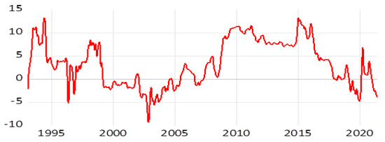
Figure 8.
Volatility spillover from oil price to foreign liabilities.
Figure 9 shows the volatility spillover from oil prices to foreign assets. Oil price was the net transmitter in the periods of 1993–2002 and 2006–2018. Interestingly, we observes oil prices as the net receiver in 2003–2004 and during the first wave of the COVID-19 pandemic. During the COVID-19 pandemic, oil prices experienced a significant plunge, eventually turning into negative oil prices.
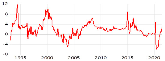
Figure 9.
Volatility spillover from oil price to foreign asset.
Apparently, the pegged exchange rate facilitated the oil export industry by stabilizing the exchange rate. Because the devaluation of the SAR would allow for the exporting sectors to earn more local currencies, it would, however, be counterproductive towards the import sectors. Nevertheless, if the United Kingdom followed the floating exchange rate, the real effective exchange rate would be devalued, implying that the devolution of the local currency promoted nonoil GDP. Our findings corroborated several existing studies that observed that the banking sector was sensitive to the internal oil price in the context of oil-exporting countries [33,34].
4. Conclusions
Saudi Arabian, characterized as a hydrocarbon economy, has enjoyed a notable resource rent under a pegged exchange system. The current study is a pioneer in measuring the dynamic response of external assets and liabilities of banks to the international oil price under different economic circumstances in the context of Saudi Arabia. Through this, we applied sophisticated frameworks, including cross-quantilogram, quantile-on-quantile, and TVP-VAR approaches, to analyze weekly time-series data from 1993 to 2021 due to the presence of extreme observations in the sample.
The empirical findings from the cross-quantilogram demonstrated that foreign assets and foreign liabilities responded positively to the international oil price mostly in long memory at moderate quantiles of foreign assets, liabilities, and oil price (1-year lag), since Saudi Arabia is one of the largest oil exporters. The frequency connectedness analysis showed that the Saudi Arabian economy encountered a downfall in foreign assets due to the plunge in the international oil price during the early wave of the COVID-19 pandemic. The TVP-VAR approach provided consistent results, indicating that, during the COVID-19 pandemic, the Saudi economy encountered negative net foreign assets, which occurred mainly as a significant plague of international oil prices. The findings of the cross-quantilogram and quantile-on-quantile approaches demonstrated that foreign assets and foreign liabilities responded asymmetrically to the volatilities of international oil prices under the bullish and bearish states of the market over different memories. Our findings implied that the Saudi monetary policy unit could predict the foreign assets and liabilities concerning international oil price volatility in different quantiles. For instance, the current price could facilitate the central bank of Saudi Arabia to forecast short-, medium-, and long-run foreign assets.
Our study was based on the bivariate model; thus, future studies can consider more control variables to explain the oil price and foreign assets nexus.
Author Contributions
Conceptualization, N.S. and K.S; methodology, K.S.; software, K.S.; validation, N.S., K.S.; formal analysis, K.S.; investigation, K.S.; resources, N.S.; data curation, N.S.; writing—original draft preparation, K.S.; writing—review and editing, K.S.; visualization, K.S.; supervision, N.S.; project administration, N.S.; funding acquisition, N.S. All authors have read and agreed to the published version of the manuscript.
Funding
Deanship of Scientific Research (DSR) at King Abdulaziz University, Jeddah, under grant no. GCV19-12-1441.
Institutional Review Board Statement
Not applicable.
Informed Consent Statement
Not applicable.
Data Availability Statement
Not applicable.
Acknowledgments
This project was funded by the Deanship of Scientific Research (DSR) at King Abdulaziz University, Jeddah, under grant no. GCV19-12-1441. The authors greatly acknowledge DSR’s technical and financial support.
Conflicts of Interest
The authors declare no conflict of interest.
References
- Bodenstein, M.; Erceg, C.J.; Guerrieri, L. Oil shocks and external adjustment. J. Int. Econ. 2011, 832, 168–184. [Google Scholar] [CrossRef]
- Bova, M.E.; Medas, M.P.A.; Poghosyan, M.T. Macroeconomic Stability in Resource-Rich Countries: The Role of Fiscal Policy; International Monetary Fund: Washington, DC, USA, 2016. [Google Scholar]
- Jibril, H.; Chaudhuri, K.; Mohaddes, K. Asymmetric oil prices and trade imbalances: Does the source of the oil shock matter? Energy Policy 2020, 137, 111100. [Google Scholar] [CrossRef]
- Kilian, L.; Rebucci, A.; Spatafora, N. Oil shocks and external balances. J. Int. Econ. 2009, 772, 181–194. [Google Scholar] [CrossRef]
- Le, T.-H.; Chang, Y. Oil price shocks and trade imbalances. Energy Econ. 2013, 36, 78–96. [Google Scholar] [CrossRef]
- Lopez-Murphy, P.; Villafuerte, M. Fiscal policy in oil producing countries during the recent oil price cycle. IMF Work. Pap. 2010, 1–23. [Google Scholar]
- Rafiq, S.; Sgro, P.; Apergis, N. Asymmetric oil shocks and external balances of major oil exporting and importing countries. Energy Econ. 2016, 56, 42–50. [Google Scholar] [CrossRef]
- Backus, D.K.; Crucini, M.J. Oil prices and the terms of trade. J. Int. Econ. 2000, 501, 185–213. [Google Scholar] [CrossRef]
- Baek, J. An asymmetric approach to the oil prices-trade balance nexus: New evidence from bilateral trade between Korea and her 14 trading partners. Econ. Anal. Policy 2020, 68, 199–209. [Google Scholar] [CrossRef]
- Fratzscher, M.; Schneider, D.; Van Robays, I. Oil prices, exchange rates and asset prices. ECB Work. Pap. 2013. [Google Scholar] [CrossRef]
- Sim, N.; Zhou, H. Oil prices, US stock return, and the dependence between their quantiles. J. Bank. Financ. 2015, 55, 1–8. [Google Scholar] [CrossRef]
- Nasir, M.A.; Naidoo, L.; Shahbaz, M.; Amoo, N. Implications of oil prices shocks for the major emerging economies: A comparative analysis of BRICS. Energy Econ. 2018, 76, 76–88. [Google Scholar] [CrossRef]
- Yildirim, Z.; Arifli, A. Oil price shocks, exchange rate and macroeconomic fluctuations in a small oil-exporting economy. Energy 2021, 219, 119527. [Google Scholar] [CrossRef]
- Hathroubi, S.; Aloui, C. Oil price dynamics and fiscal policy cyclicality in Saudi Arabia: New evidence from partial and multiple wavelet coherences. Q. Rev. Econ. Financ. 2020, 85, 149–160. [Google Scholar] [CrossRef]
- Allegret, J.P.; Mignon, V.; Sallenave, A. Oil price shocks and global imbalances: Lessons from a model with trade and financial interdependencies. Econ. Model. 2015, 49, 232–247. [Google Scholar] [CrossRef]
- Balli, E.; Çatık, A.N.; Nugent, J.B. Time-varying impact of oil shocks on trade balances: Evidence using the TVP-VAR model. Energy 2021, 217, 119377. [Google Scholar] [CrossRef]
- Eryiğit, M. The dynamical relationship between oil price shocks and selected macroeconomic variables in Turkey. Econ. Res.-Ekon. Istraž. 2012, 25, 263–276. [Google Scholar] [CrossRef]
- Gnimassoun, B.; Joëts, M.; Razafindrabe, T. On the link between current account and oil price fluctuations in diversified economies: The case of Canada. Int. Econ. 2017, 152, 63–78. [Google Scholar] [CrossRef]
- Gomes, G.; Hache, E.; Mignon, V.; Paris, A. On the current account-biofuels link in emerging and developing countries: Do oil price fluctuations matter? Energy Policy 2018, 116, 60–67. [Google Scholar] [CrossRef]
- Huntington, H.G. Crude oil trade and current account deficits. Energy Econ. 2015, 50, 70–79. [Google Scholar] [CrossRef]
- Long, S.; Liang, J. Asymmetric and nonlinear pass-through of global crude oil price to China’s PPI and CPI inflation. Econ. Res.-Ekon. Istraž. 2018, 31, 240–251. [Google Scholar]
- Özlale, Ü.; Pekkurnaz, D. Oil prices and current account: A structural analysis for the Turkish economy. Energy Policy 2010, 388, 4489–4496. [Google Scholar] [CrossRef]
- Okolo, C.V.; Udabah, S.I. Oil price and exchange rate volatilities: Implications on the cost of living in an OPEC member country—Nigeria. OPEC Energy Rev. 2019, 43, 413–428. [Google Scholar] [CrossRef]
- Varlik, S.; Berument, M.H. Oil price shocks and the composition of current account balance. Cent. Bank Rev. 2020, 201, 1–8. [Google Scholar] [CrossRef]
- Han, H.; Linton, O.; Oka, T.; Whang, Y.-J. The cross-quantilogram: Measuring quantile dependence and testing directional predictability between time series. J. Int. Econ. 2016, 1931, 251–270. [Google Scholar] [CrossRef]
- Antonakakis, N.; Gabauer, D. Refined Measures of Dynamic Connectedness Based On TVP-VAR. 2017. Available online: https://mpra.ub.uni-muenchen.de/78282/1/MPRA_paper_78282.pdf (accessed on 29 September 2022).
- Koop, G.; Korobilis, D. A new index of financial conditions. Eur. Econ. Rev. 2014, 71, 101–116. [Google Scholar] [CrossRef]
- Koop, G.; Pesaran, M.H.; Potter, S.M. Impulse response analysis in nonlinear multivariate models. J. Econ. 1996, 741, 119–147. [Google Scholar] [CrossRef]
- Sohag, K.; Gainetdinova, A.; Hammoudeh, S.; Shams, R. Dynamic Connectedness among Vaccine Companies’ Stock Prices: Before and after Vaccines Released. Mathematics 2022, 10, 2812. [Google Scholar] [CrossRef]
- Diebold, F.X.; Yılmaz, K. On the network topology of variance decompositions: Measuring the connectedness of financial firms. J. Int. Econ. 2014, 1821, 119–134. [Google Scholar] [CrossRef]
- Pesaran, H.H.; Shin, Y. Generalized impulse response analysis in linear multivariate models. Econ. Lett. 1998, 581, 17–29. [Google Scholar] [CrossRef]
- Chandrarin, G.; Sohag, K.; Cahyaningsih, D.S.; Yuniawan, D.; Herdhayinta, H. The response of exchange rate to coal price, palm oil price, and inflation in Indonesia: Tail dependence analysis. Resour. Policy 2022, 77, 102750. [Google Scholar] [CrossRef]
- Mezghani, T.; Boujelbène, M. The contagion effect between the oil market, and the Islamic and conventional stock markets of the GCC country: Behavioral explanation. Int. J. Islam. Middle East. Financ. Manag. 2018, 11. [Google Scholar] [CrossRef]
- Wang, R.; Luo, H.R. Oil prices and bank credit risk in MENA countries after the 2008 financial crisis. Int. J. Islam. Middle East. Financ. Manag. 2020, 13, 219–247. [Google Scholar] [CrossRef]


Publisher’s Note: MDPI stays neutral with regard to jurisdictional claims in published maps and institutional affiliations. |
© 2022 by the authors. Licensee MDPI, Basel, Switzerland. This article is an open access article distributed under the terms and conditions of the Creative Commons Attribution (CC BY) license (https://creativecommons.org/licenses/by/4.0/).