A Survey on Tools and Techniques for Localizing Abnormalities in X-ray Images Using Deep Learning

Abstract

Deep learning is expanding and continues to evolve its capabilities toward more accuracy, speed, and cost-effectiveness. The core ingredients for getting its promising results are appropriate data, sufficient computational resources, and best use of a particular algorithm. The application of these algorithms in medical image analysis tasks has achieved outstanding results compared to classical machine learning approaches. Localizing the area-of-interest is a challenging task that has vital importance in computer aided diagnosis. Generally, radiologists interpret the radiographs based on their knowledge and experience. However, sometimes, they can overlook or misinterpret the findings due to various reasons, e.g., workload or judgmental error. This leads to the need for specialized AI tools that assist radiologists in highlighting abnormalities if exist. To develop a deep learning driven localizer, certain alternatives are available within architectures, datasets, performance metrics, and approaches. Informed decision for selection within the given alternative can lead to batter outcome within lesser resources. This paper lists the required components along-with explainable AI for developing an abnormality localizer for X-ray images in detail. Moreover, strong-supervised vs weak-supervised approaches have been majorly discussed in the light of limited annotated data availability. Likewise, other correlated challenges have been presented along-with recommendations based on a relevant literature review and similar studies. This review is helpful in streamlining the development of an AI based localizer for X-ray images while extendable for other radiological reports.

1. Introduction

Chest X-ray (CXR) is one of the most common methods for diagnosing lung diseases among radiologists. To assist radiologists in their diagnosing tasks, researchers have proposed computer aided diagnosis (CAD) systems since 1970s [1]. They are intended to minimize the risk of false negative cases while improve the speed of diagnoses [2]. Initially, rule-based systems were considered for CAD, which were based on if-then rules. The rule-based approach became limited with the expansion of use-cases, level of complexity, and unstructured data. Thus, the trend shifted toward data mining by 1990s [3]. Now, with the rise of big-data and computational resource availability, the focus is of research tends toward machine learning for achieving excellence in CAD area.

Machine learning became a de-facto approach that learns diagnosis patterns from the data without coding explicit if–then rules. This approach requires suitable data in terms of quality and quantity with the appropriate use of a learning algorithm. The classical machine learning algorithms for the past five decades achieve better performance for lower complexity tasks within structured data [4]. However, they become inefficient for complex unstructured data, e.g., for image analysis, classification, object detection, and segmentation. This presents the need for the more advanced machine learning sub-field called deep learning.

Deep learning has outperformed in all vision tasks for non-medical images for the past ten years. For medical images, the state-of-the-art techniques in deep learning have also achieved human expert level performance in diagnosing certain abnormalities in dermatology, cardiology, and radiology.

One of the main reasons for such outstanding results is the acquisition of labeled data. Labeled data comprise two parts i.e., image and tag. For X-ray image, abnormality tag can be normal, pneumonia, or cardiomegaly. Furthermore, the tag (also refers to label or annotation) may contain limited or extended information about the image. For instance, classification task requires only label, while detection requires additional information like x, y, width, and height of the target object. This becomes even richer when dealing with segmentation tasks where pixel level segregation is the target.

Alongside classification, practitioners prefer assistance in highlighting the abnormalities [5,6,7] from CAD system as a second opinion [5]. Such highlights better assist physicians toward diagnosing conclusions. This is also desirable to overcome false negative cases. According to the literature, deep learning has established a good reputation for medical image classification [6], bounding box formation [7], and segmentation [8]. Research in deep learning through medical images confronts many challenges [9,10]. Availability of quality data in large volume, no-interpretability, resource (memory, speed, space) management, and hyperparameter selection are some major bottlenecks, among many [11].

There exist brief discussions on state-of-the-art image classification models from generic to medical perspectives. For instance, [9,12,13,14] provided in depth details about the deep learning architectures, their strengths, and challenges in general. A good deal of literature, including [15,16,17,18,19], discuss stated architectures for medical image analysis. The focus of these efforts is around classification and prediction at image level [14]. For localization with bounding box and segmentation, Refs. [6,7,15,16,17,18,19,20,21] have provided brief details for X-ray images. For instance, in survey [6], several articles regarding the application of deep learning on chest radiographs were examined that were published prior to March 2021. They included publicly available datasets, together with the localization, segmentation, and image-level prediction techniques. Another study [17] mainly focused on techniques based on salient object detection while highlighted challenges in the area. To the best of our knowledge, very little discussions are available in the literature that address challenges for weak supervised learning in explainable AI perspective. Furthermore, class activation mapping has forged a new branch that offers interpretable modeling while capability for localization as biproduct. The primary focus of this paper is to explore the approaches that overcome the need for rich-labeled data acquisition and enhancing the interpretability of results for medical images. To date, the best results have been reported with supervised learning [9] where training data are labelled with rich information like class label, box labels (x, y, width, height) and/or masked data). The acquisition of such labels for medical images is expensive to generate in terms of time and efforts. Furthermore, the deep learning models, trained on such annotations are not interpretable enough for human inspection [11,22]. Subject matter specialists (SME) often require debugging the learnt deficiencies for optimization. Such analysis is performed without knowing how the model generated the output from a given input. Without interpretability, the model stays black-box and may endure bias leading to skewed decisions.

Approaches to detect objects without strong annotation are referred to as weak-supervised learning. They leverage image-level class labels to infer localization by heatmaps, saliency-maps, or attentions. We observed the growing trend toward weak-supervised learning techniques for localizing medical images. Recently, class activation map (CAM) -based approaches [23,24,25,26,27,28,29,30,31,32,33] have gained popularity in deep learning, offering (1) interpretability and (2) weak-supervised driven localization. They comprise sufficient information to constitute bounding-box and segmented regions. In this research, we explore deep learning approaches that offer the best performance for classification, localization, and interpretability in more generic form using medical image toward diagnosis.

The rest of the paper is organized in generic to specific order. A generic background has been presented in Section 2 about deep learning and its evolution from shallow artificial neural network to deeper architectures like convolution neural networks. Section 3 illustrates the metrics for the performance evaluation of the deep learning models. In Section 4, datasets for chest X-ray have been discussed in brief. Using the given datasets, most common state-of-the-art classification and localization approaches have been discussed for supervised learning in Section 5. Since supervised learning demands rich labels, whose availability is challenging in larger volume, weak supervised approaches become next choice for localization. Section 6 describes weak supervised learning approaches for localization in the context of medical applications. Based on literature reviews and available options, some gaps and challenges have been observed, as listed in Section 7 along with recommendations.

2. Background

Deep learning is a machine learning approach that primarily uses artificial neural networks (ANN) as a principal component. ANN simulates the human brain system to solve general learning problems. However, between 1980s and 1990s, it was equipped with a back-propagation algorithm [34] for learning, but remained out-of-practice due to the unavailability of suitable data and computational resources. With the advancement of parallel computing and GPU technology, it gained popularity in the 2000s to become a de-facto approach in machine learning.

At its very basic, deep learning teaches a computer how to wire input with output via hidden layers for predictions based on training data. Prediction can be made for many tasks, e.g., regression, classification, object detection, segmentation, etc.

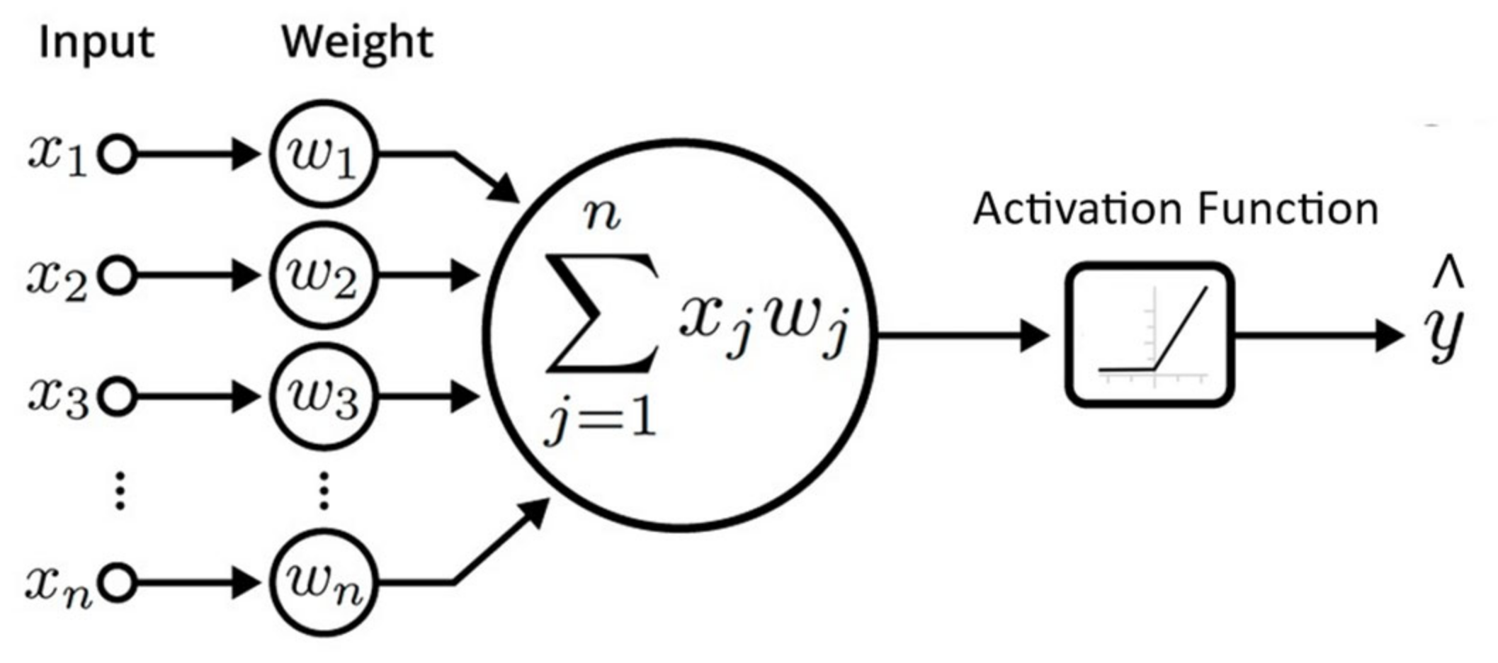
2.1. Artificial Neural Network

Artificial neurons represent a set of interconnected units or nodes that serve as the foundation of an ANN and are meant to mimic the function of biological brain neurons. Each artificial neuron contains inputs and generates a single output that can be transmitted to numerous other neurons (see Figure 1). The input X ∈ x₁, x₂, x₃, …, x_n is weighted with a learnable parameter W ∈ w₁, w₂, w₃, …, w_n. Their dot product is first aggregated and then one of the activation functions, e.g., tanh, sigmoid, ReLU, etc., is applied. In the training phase, the outcome of activation function is compared with actual label. The difference is backpropagated to update the W as per delta. This process is repeated for the whole dataset multiple times until the difference between activation function and actual label reaches the minimum possible value.

2.2. Multilayer Perceptron

Deep learning architectures can be formed by embedding the artificial neurons into multiple hidden layers. Adding more hidden layers makes the architecture deeper, increasing the possibility of better performance. Figure 2 illustrates a three (hidden) layer deep learning architecture that is called multilayer perceptron (MLP). This kind of architecture is expensive in terms of computational resources. Therefore, they are altered in many ways, e.g., dropping-out connections, reduction in neurons in hidden layers, etc.

MLPs are useful in classification and regression tasks for structured data. However, they cannot perform well on unstructured data, e.g., images and sound streams.

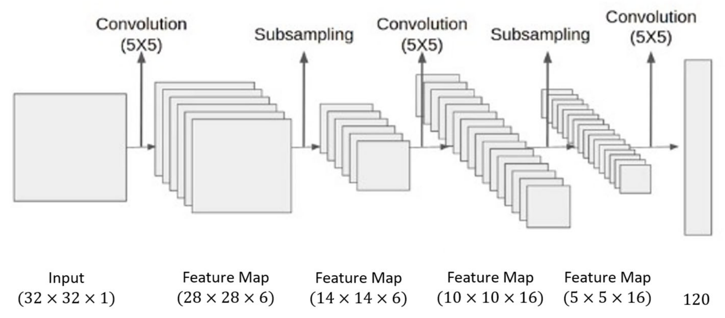
2.3. Convolutional Neural Network

The convolutional neural network (CNN) is another type of deep learning architecture that replaces the general matrix multiplication with convolution operator [12]. CNN architecture was induced by the functions of the visual cortex. Their design specializes in addressing pixel data and mostly applied in image and sound analysis tasks. The convolution operator is the core of CNN that makes them shift invariant. The convolution kernels/filters slide along input features and extract useful information in feature maps within concise space.

Pooing is another operator that is mostly used in conjunction with convolution in almost all CNN architectures. Like convolution, pooling also reduces the dimension of the feature map to make the features generalized and independent of their location in the image. However, pooling operator is fixed that is not meant to be learnt during training and contributes to reduce overfitting effects. CNN also uses some other operations to achieve better performance like dropout, batch normalization, skip connections, etc. There are many varieties in convolution base neural network architectures. The two most common approaches are end-to-end convolutional and hybrid with non-convolutional task. The end-to-end convolutional networks begin with larger resolution with one-or-three channels and end with one-by-one resolution but fatter channels (see Figure 3). The hybrid convolutional networks, use its convolutional part for feature extraction while the remaining is used for final task like classification (see Figure 4). The convolutional neural network first gained popularity when Yann LeCun created LeNet-5 for recognizing handwriting digits in 1989 [35].

This architecture consisted of 5 layers and employed a backpropagation algorithm for training. Motivated by its success, more scholars explored the approach and developed more robust CNN architectures.

Meanwhile, during the 2000s, researchers like Fei-Fei Li were working on a project called ImageNet to create a large image dataset. It crowdsourced its labeling process and initiated ImageNet challenge. The problem was to recognize object categories in common images that one can find on the Internet. The challenge became popular among the machine learning community where various approaches were adopted in competition. The classical methods hit a plateau in terms of performance. In 2012, Krizhevsky et al. ranked top with their CNN based network called AlexNet. Since then, the leaderboard has consisted of CNN models (see Figure 5).

ImageNet competitions promoted the research in deep learning architectures. They are still first choice for any image classification task. Xception [36], VGG [37], ResNet [38,39], Inception [40], MobileNet [41,42], DenseNet [43], NASNetMobile [44], and EfficientNet [45] are just a few are them that are available in Tensorflow and Pytorch as ready to use modules. Since they are capable to predict 1000 classes within daily use objects, they require too few changes to be adapted for similar domains.

One noticeable gap has been found in medical domain, when they have been adapted with ImageNet weights. In order to detect COVID-19 cases, authors have used pretrained ImageNet models i.e., MobileNetV2, NASNetMobile, and EfficientNetB1 in [46]. The same strategy has also been adapted in [47]. They used them as base models which were later fine-tuned on medical images.

Most commonly available deep learning models are available in with pre-trained weights in Tensorflow, Pytorch, Caffe2, and Matlab. Taking advantage of their availability and respective performance, we include them in our experimental setup. Based on their results within our research, they will be part of transfer and ensemble learnings.

Table 1. Popular Deep learning models trained on ImageNet for classification.

Model	Size (MB)	Top-1 Accuracy	Top-5 Accuracy	Parameters	Depth
Xception	88	0.790	0.945	22,910,480	126
VGG16	528	0.713	0.901	138,357,544	23
ResNet50	98	0.749	0.921	25,636,712	-
ResNet152V2	232	0.780	0.942	60,380,648	-
InceptionV3	92	0.779	0.937	23,851,784	159
InceptionResNetV2	215	0.803	0.953	55,873,736	572
MobileNet	16	0.704	0.895	4,253,864	88
MobileNetV2	14	0.713	0.901	3,538,984	88
DenseNet121	33	0.750	0.923	8,062,504	121
NASNetMobile	23	0.744	0.919	5,326,716	-
EfficientNetB0	29	-	-	5,330,571	-

lists popular TensorFlow architectures.

3. Method for Performance Analysis

An evaluation matrix is a key component used to gauge the performance of a machine learning model. There exist several methods that require comprehension and selection for a given task. Use of multiple metrics has widely been observed for the medical domain [48]. This section briefly discusses various performance matrixes.

3.1. Accuracy

Classification accuracy (CA) or simple classification is the basic metric that is used for gauging the performance of a classification model in machine learning. It is the ratio of number of correct predictions to the total number of input samples.

$$Accuracy=\frac{Number of Correct Predictions}{Total number of Predictions made}$$

(1)

Classification is the simplest metric that is vulnerable for giving false sense of achieving high accuracy. Other metrics illustrate more clear performance by adding the following components in their equations:

• True Positive: output that correctly indicates the presence of a condition.
• True Negative: output that correctly indicates the absence of a condition.
• False Positive: output that wrongly indicates the presence of a condition.
• False Negative: output that wrongly indicates the absence of a condition.

3.2. Precision

Precision also known as positive predictive value (PPV) refers to the proportion of positive cases that were correctly identified.

$$Precision=\frac{True Positive}{True Positive+False Pasitive}$$

(2)

3.3. Sensitivity

Sensitivity or recall is the proportion of actual positive cases which are correctly identified.

$$Sensitivity=\frac{True Positive}{True Positive+False Negative}$$

(3)

3.4. Specificity

Specificity is the proportion of actual negative cases which are correctly identified.

$$Precision=\frac{True Negative}{True Negative+False Positive}$$

(4)

3.5. Jaccard Index

Jaccard index is also known as intersection over union (IoU). Almost all object detection algorithms (i.e., bounding box) consider IoU as core evaluator. It is defined over sets as (Intersection between two sets)/(Union of two sets).

$Jacard Index=\frac{Area of Overlap}{Area of Union}$

(5)

In computer vision, it evaluates the overlap between two bounding boxes. The keynote for IoU in weak surprised learning is the unavailability of ground truth values. This makes it challenging to validate the performance of given model. Among alternatives, one way to quantify model performance on IoU can be the use of ground truth values for smaller testset. Such a testset can be taken from the same distribution and annotated by field experts, e.g., a radiologist. Another option could be the application of the same model on another domain’s rich annotated dataset where ground truth information may not be exposed or used during training but only for validation and testing.

3.6. Evaluation Matrix for Medical Diagnosis

In medical diagnosis, the cost of failing to diagnose the fatal disease of a sick person is much higher than the cost of sending a healthy person to more tests. Therefore, specificity and sensitivity are most suitable matrices when it comes to classification tasks.

4. Chest X-ray Datasets

Deep learning performs best on large volume of data. With the digitization technologies, medical institutions can collect radiographs in large volume. Alongside, researchers have extracted the textual reports associated with the radiographs and applied natural language processing (NLP) to categorized them for further research [49]. The use of computer aided labeling tools have also enabled data preparation at faster pace, e.g., LabelMe LabelImg, VIA, ImageTagger [50]. For instance, Snorkel [51] offers intelligence in generating masks for segmentation tasks with limited human supervision. Using some of these facilities, X-ray datasets with a large number of images have been formed for research purposes.

Some of the most cited datasets have been illustrated in

Table 2. Popular Chest X-ray datasets.

Initiator	Name	Total	Frontal View	Geographic
National Institute of Health	ChestX-ray8	112,120	112,120	Northeast USA
Stanford University	CheXpert	223,141	191,010	Western USA
University of Alicante	PadChest	160,868	67,000	Spain
VinBrain	VinDr-CXR	15,000	15,000	Vietnam
National Library of Medicine	Tuberculosis	800	800	China + USA

. With the formation of large datasets, e.g., ChestXray8 [49], CheXpert [52], and VinDr-CXR [53], deep learning became sufficiently trainable for better performance.

4.1. ChestXray8

ChestXray8 [49] consists of 112,120 chest radiographs from 30,805 patients collected between 1992 and 2015. They were collected at National Institute of Health (Northeast USA). Each CXR is an 8-bit grayscale image having 1024 × 1024 pixels that can have multiple labels. NLP was applied on their associated reports to label them within 14 types of abnormalities.

The dataset also includes 880 hand labeled bounding box labels for localization. Some CXR images have more than one B.Boxes that makes 984 labels in total. Only eight out of 14 disease types were marked for BBox annotation. Figure 6 illustrates sample images for some classes. Without much manual annotation, this dataset poses some issues regarding the quality of its labels [54].

4.2. CheXpert

CheXpert [52] dataset was formed by Stanford Hospital that consists of 224,316 chest radiographs from 65,240 unique patients. The images were collected between 2002 and 2017 that spans within 12 abnormalities (see Figure 7). Each image is 8-bit grayscale with no change in original resolution.

The dataset was annotated using a rule-based labeler from radiology report that specified the absence, presence, uncertainty, and no-mention of 12 given abnormalities.

4.3. CheXpert

PadChest [55] dataset contains 160,868 images from 67,000 patients. It was created at San Juan Hospital (Spain) within 2009 and 2017. The images are in original resolution with 16-bit grayscale. The annotation for these images were created in two step process. First, a small portion of 27,593 images were manually labeled by a group of physicians. Using these labels, in a second step, an attention based RNN was trained to annotate the rest of the dataset. The labeled images were then evaluated against a hierarchical taxonomy that is based on UML standard.

4.4. VinDr-CXR

VinDr-CXR [53] dataset was created from the images collected from two of the Vietnam’s largest hospitals i.e., Hospital-108 and the Hanoi Medical University Hospital. They followed three step process to generate the database. First, data were collected from the hospitals between 2018 and 2020. Secondly, data were filtered to remove outliers such as images of body parts other than chest. Lastly, the annotation step was executed. It consists of 15,000 CXRs, out of which 18,000 were manually annotated by a group of 17 experienced radiologists with the classification and localization of 22 common thoracic diseases.

4.5. Montgomery County and Shenzhen Set

The Montgomery County and Shenzhen set [56] dataset consists of two CXR datasets produced by the U.S. National Library of Medicine. The Montgomery County (MC) contains manually segmented lung masks offers a benchmark for the evaluation of automatic lung segmentation methods. It has 138 X-ray radiographs, out of which 58 are TB positive cases. They were collected in collaboration with the Department of Health and Human Services, Montgomery County, Maryland (USA). The radiographs are 12-bit grayscale with either 4020 × 4892 or 4892 × 4020 pixels. The Shenzhen dataset contains 662 CXRs, including 335 cases with manifestations of TB. They were collected in collaboration with Shenzhen No.3 People’s Hospital, Guangdong Medical College, Shenzhen, China. The images are in PNG format with 3000 × 3000 pixels resolution. The datasets offer segmented masks of lungs in finer quality, making it a nice candidate for test or validation sets.

4.6. JSRT Database

The JSRT database [57] was developed by the Japanese Society of Radiological Technology. It comprises 154 CXRs with lung nodule. Out of these nodules, 100 are malignant while 54 are benign. Each image is 12-bit, 4096 gray scale 2048 × 2048 matrix size, 0.175 mm pixel size. The lung nodule images have been divided into 5 groups according to the degrees of subtlety. Moreover, nodule location information has also been added with X and Y coordinates. This dataset is though small but still useful for research and educational purpose. The application of classical machine learning methods is feasible, but deep learning may not be a useful approach.

4.7. JSRT Database

MIMIC-CXR [58] is a CXR dataset containing 371,920 images from 64,588 patients. The radiographs have been collected from emergency department of Beth Israel Deaconess Medical Center between 2011 and 2016. The images are 8-bit grayscale in full resolution and labelled using a rule-based labeler from associated reports.

The dataset quoted above are obviously not an exhaustive list of available datasets. They are mostly cited and publicly available till to date. Furthermore, they have been included in this report to cover the breadth of their kind. For instance, Montgomery, Shenzhen, JSRT offered rich annotations for segmentation [56,57,58]. Other noticeable datasets, e.g., PadChest [55], VinDr-CXR [53], Tuberculosis [56], and Kaggle [17], contributed in data diversity. They, along with others [19,59], created a sound benchmark for weak supervised driven localization over heatmaps, bounding box, and segmentation [7,60,61,62,63]. The major gap can be observed in interoperability of models for the datasets. A model that is trained, validated, and tested on one dataset was not reported valid on same domain’s other dataset. We would refer this gap as lack of domain sharing. If a COVID-19 classifier (model) performs 90% well on dataset-A, then it should achieve near level performance on dataset-B of similar domain.

5. Diagnosis Using Chest Radiographs

Detecting the signs of symptoms in X-ray images has been widely studied [54,62,64]. Deep learning methodologies in this area have demonstrated their value for localization and classification [64]. The fuel for such advancement were the availability of large size datasets and computational resources. This encouraged researchers to design deeper and wider deep learning architectures [37]. Some architectures became more popular because of their general-purpose offering irrespective to a specific domain [9].

Medical diagnosis is the most sensitive area where precision and reliability are the key requirements for any CAD system [3]. A patient with positive abnormal conditions must be captured even with slight chances.

In Figure 8, we illustrate a taxonomy of deep learning approaches that can be used for object detection and segmentation from the literature. This taxonomy can also be considered when planning to develop or train a localizer for medical images like X-ray images. Strong supervision, as explained in Section 5.1, shall be highly preferred if the given dataset contains all the required ground truth information. For such instances, all classification tasks must be executed with a strong supervised approach. The same approach shall also be carried out for object detection and segmentation when rich annotated information is available. However, most datasets in the medical domain may not contain required spatial information. For such scenarios, weak supervision can be considered.

This section briefly discusses the trends in medical diagnosis using deep learning in general while keeping the focus on localization. The first subsection highlights deep learning methods from supervised learning that deal with image-level prediction and localization. The next subsection discusses the same tasks in weak supervised learning.

5.1. Classification and Localization Using Supervised Learning

A dense volume of literature has highlighted the strengths of supervised learning in classification and localization using deep learning [9,13,21]. Formally, supervised learning refers to a task that learns f: X → Y from a training data set D = $\left\{\left(x_1, y_1\right), \dots , \left(x_m, y_m\right)\right\}$, where X is the feature space, Y = {$c_1, c_1,\dots , c_k$}, $x_i$ ∈ X, and $y_i$ ∈ Y. Assuming, $\left(x_i, y_i\right)$ are generated according to an unknown independent and identical distribution $D$. In this approach, the predictive models are constructed by learning from a large number of training examples, where each example has at least one label that indicates its ground-truth output [65].

Deep learning has achieved top ranking performance in classification tasks with supervised learning. In the context computer vision, classification is also known as image-level prediction. In this task, trained model predicts labels by analyzing an entire image. The reason behind such performance is the availability of data that encouraged the researchers to experiment with sophisticated deep learning architectures even if they are computationally expensive. For image level prediction, the training dataset requires semantic organization like sub-division into classes. This opens new chapters of challenges, e.g., class-imbalance, missing labeling, incorrect labeling, generalization, and more. To deal with all or some of these challenges, various methodologies have been proposed. Table 3 summarizes some of such efforts that were made in the past three years.

Similar to classification at the image level, the localization task has also gained attention in the past decade using deep learning [66,67]. Localization refers to the task of highlighting the area-of-interest within an image either with bounding box, segmented contour, heatmap, or segmentation mask. In medical diagnosis, classification without localization answers half of the question [10]. Medical practitioners expect assistance not only at the radiograph level with abnormality detection, but also to visualize the signs and location. This requirement has been addressed in the literature by drawing BBox or segmentation. The associated challenge is the acquisition of rich dataset that is extended beyond image level annotation. For BBox task, each image must have x, y, width, and height. Likewise, segmentation task requires mask as annotation data. There also exist some ground-truth labels for BBox or segmentation in the listed datasets (see Table 2). Leveraging these annotations with combination to specialized networks and pre and post processing [14], some literature has been included in Table 3.

Object detection and segmentation techniques use various approaches to overcome data, computation, and performance bottlenecks. In these techniques, object detection and localization are either performed in two stages or one.

5.2. R-CNN

Ross Grishick et al. proposed R-CNN [68] that performs object detection in two stages. First, multiple regions are extracted and proposed using selective search [69] in bottom-up flow. CNN extracts feature from the candidate regions that are fed into an SVM to classify the presence of the object within that candidate region proposal. Moreover, it also predicts four values of the bounding box, which are offset values to increase the precision. The problems with R-CNN are longer training and prediction time. Its selective search also lacks the ability to learn that causes bad proposal generations.

5.3. SPP-Net

SPP-Net [70] was introduced right after R-CNN. The SPP-Net managed the model agnostic of input image size that improved the prediction speed of bounding box as compared to the R-CNN, without compromising on the mAP. Spatial pyramid pooling was used in the last layer of their network. This removed the fixed-size constraint of the network.

5.4. Fast R-CNN

To overcome the limitations of R-CNN, Ross Grishick et al. built Fast R-CNN [71]. Instead of feeding the proposed regions to the CNN, a convolutional feature map was generated from the input image. It helped in identification of right region. This approach significantly reduced the training time. For prediction at test stage, region proposal task was still an issue that required further improvements.

Table 3. List of popular Techniques for Classification and Localization using Weak Supervised Learning.

S.No	Ref No	Methodology	Dataset
1	[72]	Using lung cropped CXR model with a CXR model to improve model performance	ChestX-ray14 JSRT + SCR,
2	[73]	Use of image-level prediction of Cardiomegaly and application for segmentation models	ChestX-ray14
3	[74]	Classification of cardiomegaly using a network with DenseNet and U-Net	ChestX-ray14
4	[75]	Employing lung cropped CXR model with CXR model using the segmentation quality	MIMIC-CXR
5	[76]	Improving Pneumonia detection by using of lung segmentation	Pneumonia
6	[77]	Segmentation of pneumonia using U-Net based model	RSNA-Pneumonia
7	[78]	To find similar studies, a database has been used for the intermediate ResNet-50 features	Montgomery, Shenzen
8	[79]	Detection and localization of COVID-19 through various networks and ensembling	COVID
9	[80]	GoogleNet has been trained with CXR patches and correlates with COVID-19 severity score	ChestX-ray14
10	[81]	A segmentation and classification model proposed to compare with radiologist cohort	Private
11	[82]	A CNN model proposed for identification of abnormal CXRs and localization of abnormalities	Private
12	[83]	Localizing COVID-19 opacity and severity detection on CXRs	Private
13	[84]	Use of Lung cropped CXR in DenseNet for cardiomegaly detection	Open-I, PadChest
14	[85]	Applied multiple models and combinations of CXR datasets to detect COVID-19	ChestX-ray14 JSRT + SCR, COVID-CXR
15	[86]	Multiple architectures evaluated for two-stage classification of pneumonia	Ped-pneumonia
16	[87]	Inception-v3 based pneumoconiosis detection and evaluation against two radiologists	Private
17	[88]	VGG-16 architecture adapted for classification of pediatric pneumonia types	Ped-pneumonia
18	[89]	Used ResNet-50 as backbone for segmentation model to detect healthy, pneumonia, and COVID-19	COVID-CXR
19	[90]	CNN employed to detect the presence of subphrenic free air from CXR	Private
20	[91]	Binary classification vs One-class identification of viral pneumonia cases	Private
21	[92]	Applied a weighting scheme to improve abnormality for classification	ChestX-ray14
22	[93]	To improve image-level classification, a Lesion detection network has been employed	Private
23	[94]	An ensemble scheme has been used for DenseNet-121 networks for COVID-19 classification	ChestX-ray14

Table 3. List of popular Techniques for Classification and Localization using Weak Supervised Learning.

S.No	Ref No	Methodology	Dataset
1	[72]	Using lung cropped CXR model with a CXR model to improve model performance	ChestX-ray14 JSRT + SCR,
2	[73]	Use of image-level prediction of Cardiomegaly and application for segmentation models	ChestX-ray14
3	[74]	Classification of cardiomegaly using a network with DenseNet and U-Net	ChestX-ray14
4	[75]	Employing lung cropped CXR model with CXR model using the segmentation quality	MIMIC-CXR
5	[76]	Improving Pneumonia detection by using of lung segmentation	Pneumonia
6	[77]	Segmentation of pneumonia using U-Net based model	RSNA-Pneumonia
7	[78]	To find similar studies, a database has been used for the intermediate ResNet-50 features	Montgomery, Shenzen
8	[79]	Detection and localization of COVID-19 through various networks and ensembling	COVID
9	[80]	GoogleNet has been trained with CXR patches and correlates with COVID-19 severity score	ChestX-ray14
10	[81]	A segmentation and classification model proposed to compare with radiologist cohort	Private
11	[82]	A CNN model proposed for identification of abnormal CXRs and localization of abnormalities	Private
12	[83]	Localizing COVID-19 opacity and severity detection on CXRs	Private
13	[84]	Use of Lung cropped CXR in DenseNet for cardiomegaly detection	Open-I, PadChest
14	[85]	Applied multiple models and combinations of CXR datasets to detect COVID-19	ChestX-ray14 JSRT + SCR, COVID-CXR
15	[86]	Multiple architectures evaluated for two-stage classification of pneumonia	Ped-pneumonia
16	[87]	Inception-v3 based pneumoconiosis detection and evaluation against two radiologists	Private
17	[88]	VGG-16 architecture adapted for classification of pediatric pneumonia types	Ped-pneumonia
18	[89]	Used ResNet-50 as backbone for segmentation model to detect healthy, pneumonia, and COVID-19	COVID-CXR
19	[90]	CNN employed to detect the presence of subphrenic free air from CXR	Private
20	[91]	Binary classification vs One-class identification of viral pneumonia cases	Private
21	[92]	Applied a weighting scheme to improve abnormality for classification	ChestX-ray14
22	[93]	To improve image-level classification, a Lesion detection network has been employed	Private
23	[94]	An ensemble scheme has been used for DenseNet-121 networks for COVID-19 classification	ChestX-ray14

5.5. Faster R-CNN

R-CNN [68] and Fast R-CNN [69] both used selective search [69] for creating region proposals, which was slowing-down the network performance. This shortcoming was identified and fixed by Shaoqing Ren et al. in Faster R-CNN [95]. They replaced the selective search with object detection algorithm. This enabled the network to learn the region proposal.

Among the two staged networks, Faster R-CNN was the fastest as can be observed in Figure 9.

5.6. YOLO

Joseph Redmon et al. designed YOLO (You Only Look Once) [96] in 2015, a single shot object detection network. Its single convolutional network predicts the bounding boxes and the class probabilities. YOLO has gained popularity for its superior performance over the previous two-shot object detection techniques. The model divides the input image into grids and computes the probabilities of an object inside each grid. Next, it combines nearby high-value probability grids as single object. Using non-max suppression (NMS), low-value predictions are ignored. During training, the center of each object is detected and compared with the ground truth, where weights are adjusted according to the delta. In subsequent years, multiple improvements have been made to the architecture and released in successive versions, i.e., YOLOv2 [97], YOLOv3 [98], YOLOv4 [99], and YOLOv5 [100].

5.7. SSD

As the name describes, single shot detector (SSD) [101] takes a single shot for detecting multiple objects within the input image. It was designed by Wei Liu et al. in 2016 and combines Faster R-CNN (anchor approach) and YOLO (one-step structure) key capabilities to perform faster and with greater accuracy. Furthermore, SSD employed VGG-16 as a backbone and adds four more convolutional layers to form the feature extraction network. Performance of SSD300 has been reported 74.3% mAP at 59 FPS. Similarly, SSD500 achieves 76.9% mAP at 22 FPS, outperforming Faster R-CNN and YOLOv1 at sound margins.

6. Localization Using Weak-Supervised Learning

The localization task requires more processing efforts and resources as compared to image-level classification. Supervised learning is indeed a first-to-try approach to deal with it. However, the major challenge for supervised learning is the acquisition of required annotation. This becomes worse for medical imaging for the fact that the labeler must generally be a medical professional [60]. For the large volume of correct annotation, the task becomes too expensive in terms of time and cost.

Table 4. Summary of Weak Supervised based Deep Learning approaches for object detection.

Approach	Variants	Description
Class Activation Maps	Grad-CAM	Weight the 2-Dimension activations by averaging gradients
	Score-CAM	Perburate the input image by scaling activations to estimate how the output drops
	Full-Grad	Calculates the biases’ gradients from all over the network before summing them
Attention models	RAN	In Residual Attention Networks, several attention modules have been employed to the backbone network for learning the mask in each convolutional layer
	ADL	Attention based Dropout Layer utilizes the self-attention to process the feature maps of the model
	STN	Spatial Transformation Network explicitly allows the spatial manipulation of data within the CNN.
Saliency Maps	ISL	Image Level Supervision first classifier is trained with foreground features and then generate saliency maps in top-down scheme.
	DUS	Deep Unsupervised Saliency that works collaboratively with a latent saliency prediction module and a noise modeling module.
	C2S	Contour2Saliency exploits a coarse-to-fine architecture that generates saliency maps and contour maps simultaneously

outlines various alternatives within weak supervised approaches for localization.

As an alternative to supervised learning where acquisition of BBox or segmented masks are not feasible, weak supervision can play a vital role. Learning with weak supervision involves learning from incomplete, inexact, or inaccurate labels. Weakly supervised learning for predictive models learn about the task (e.g., BBox detection) indirectly from noisy or incomplete labels [65]. In this work, we explore three main classes of weak supervised driven localization called class activation maps, attention models, and saliency.

Addition to the approaches given in Figure 8 and Table 4, there exist other techniques that have shown better feasibility for localization. For instance, self-taught object localization by masking out image regions has been proposed to identify the regions that cause the maximal activations to localize objects [102]. Similarly, objects have been localized by combining multiple-instance learning with CNN features [103]. In [104], authors have proposed transferring mid-level image representations. They argued that some object localization can be realized by evaluating the output of CNNs on multiple overlapping patches. However, the localization abilities were not actually evaluated by these methods. Since they are not trained end-to-end, therefore requiring multiple forward passes, this makes them harder to scale to real-world datasets [28,29,30].

6.1. Class Activation Map (CAM) Based Localization

Class activation map is an effective approach for obtaining the discriminative image areas that a CNN uses to identify a certain class in the image. The aim of CAM base techniques is to produce a visual explanation map. These maps are illustrated via heatmaps that show weights for vital areas of an input image that contribute to the model’s conclusions at pixel-level. The vanilla version of CAM has emerged since 2014 and evolved in multiple variants as listed in

Table 5. Illustration of popular CAM Variants.

Variant	Mechanism
CAM	Replaced the first fully-connected layer in the image classifiers with a global average pooling layer
Grad-CAM	Weight the activations using the average gradient
Grad-CAM++	Extension of Grad-CAM that uses second order gradients
XGrad-CAM	Extension Grad-CAM that scales the gradients by the normalized activations
Ablation-CAM	Measure how the output drops after zeroing out activations
Score-CAM	Perbutate the image by the scaled activations and measure how the output drops
Eigen-CAM	Takes the first main element of the 2D activations and increases outcomes without utilizing class discrimination.
Layer-CAM	Spatially weight the activations by positive gradients. Works better especially in lower layers
Full-Grad	Computes the gradients of the biases from all over the network, and then sums them

.

6.1.1. CAM (Vanilla Version)

The idea of class based maps was inspired by global max pooling (GMP) [105]. The GMP was applied to localize an object by a single point. Their localization was limited to pointing out a target object with a single point rather than bounding the area of full object. Their work was extended in [23] by replacing GMP with global average pooling (GAP) (see Figure 10). The intuition was to take benefits from the loss for average pooling while the network identifies objects’ discriminative regions. This approach, known as class activation map (CAM), was generic enough for the network it was not trained on. CAM can be a first of its kind in identifying discriminative regions using GAP.

Though it inspired the community for its visualization idea, there are tradeoffs concerning the complexity and performance of the model. This was specifically applicable to CNN architectures whose last layer is either a GAP layer or alterable to inject GAP. For the latter case, the altered model needs retraining to adjust new layer weights.

6.1.2. Grad-CAM

The main limitation of CAM is alteration in architecture that was immediately resolved by subsequent variants. The first variant launched as Grad-CAM [29] that uses the gradients of any targeted class for producing a coarse location map (see Figure 11). To illustrate its contribution to the target class, it uses the average gradients of a feature map. This eliminates the needs of architectural modification and model retraining. Grad-CAM highlights the salient pixels in the given input image and improves the CAM’s capacity for generalization for any commercial CNN-based image classifier.

Since Grad-CAM does not rely on weighted average, the localization area corresponds to bits and parts of it instead of the entire object. This decreases its ability to properly localize objects of interest in the case of multiple occurrences of the same class. The main reason for this decrease is emphasizing the global information that local differences are vanished in it.

6.1.3. Grad-CAM++

As its name suggests, Grad-CAM++ [24] can be thought of as a generalized formulation of Grad-CAM. Likewise, it also considers convolution layer’s gradients to generate a localization map for salient regions on the image. The main contribution of Grad-CAM++ is to enhance the output map for the multiple occurrences of same object in a single image. Specifically, it emphasizes the positive influences of neurons by taking higher-order derivatives into account.

On the way forward while computing gradients, both the variants suffer from the problem of diminishing gradient when they are saturated. This causes the area of interest either missed or highlighted with too small values to be noticed. The issue becomes worse if the classifier does not earn a better reputation in terms of the accuracy metric.

6.1.4. Score-CAM

To address the limitations of gradient based variations, Score-CAM was proposed in [30]. In general, Score-CAM prefers global encoding features instead of in local ones. It works in perturbation form where mask part of regions is observed within input with respect to target score. It extracts the activations during forward pass from last convolutional layer. The resulted shape is up-sampled as per input image which are then normalized to in [0, 1] range. The normalized activation map is multiplied with original input image such that the up-sampled maps are projected to generate a mask. Lastly, the masked Image is passed to CNN with SoftMax output.

Score-CAM has been referred as post-hoc visual explainer that excludes the use of gradients. However, it pipelines of subtasks makes it computationally expensive among its class. Moreover, it usually performs well on visual comparison, but its localization results remain coarse, which further causes certain cases of non-interpretability.

6.1.5. Layer-CAM

Layer-CAM generates class activation map by taking different CNN’s layers into account [31]. It first multiplies the activation value of each location in the feature map by a weight and then combined linearly. This generates class activation maps from shallow layers. This hierarchical semantic operation makes Layer-CAM to utilize information from several levels to capture fine-grained details of target objects. This makes it easy to make it applicable to off-the-shelf CNN based classifiers without altering the network architectures and the way their back-propagation work.

Layer-CAM is an effective method to improve the resolution of the generated maps. In some cases, their quality drops due to the noise of inherited gradients. This can be overcome by finding an alternative approach from the use of gradients or suppressing the responsible noise.

6.1.6. Eigen-CAM

Eigen-CAM eliminates dependance on the backpropagation for gradients, the score of class relevance, or maximum activation locations [28]. In short, it does not rely on any form of weighting features. It calculates and displays the principal components of the acquired features from the convolutional layers. It performs well in creating the visual explanations for multiple objects in an image.

Like other variants, Eigen-CAM demands no alteration in CNN models or retraining but also excludes dependency of gradients. It is agnostic of classification layers because it just requires the learnt representations at the final convolution layer.

6.1.7. XGrad-CAM

In stated models, the authors observed insufficient theoretical support which they have attempted to address in [27]. They proposed XGrad-CAM and devised two axioms, sensitivity and conservation. The method is an extension to Grad-CAM that scales the gradients by the normalized activations. Their goal was to satisfy both the axioms as much as possible in order to make the visualization method more reliable and theoretically sound. Since the properties of these axioms are self-evident therefore, their confirmation shall make the CAM outcome more reliable. XGrad-CAM complies both the axioms’ constraints while maintaining a linear combination of feature maps.

6.1.8. Other Variants

The research community is active in class activation method enhancements and has proposed many other variants. For instance, Ablation-CAM [26] observes the impact of the output drops after zeroing out activations. Full-Grad [25] considers the gradients of the biases from all over the network, and then sums them to generate maps. Poly-CAM [33] combines earlier and later network layers to generate CAM with high resolution. Likewise, Reciprocal CAM [32] (Recipro-CAM) is a lightweight and gradient free method which extracts masks into feature maps by exploiting the correlation between activation maps and network outputs.

Table 5 list some newly and enhanced techniques of our interest. They have primarily been designed and trained for non-medical images to achieve higher accuracy in weak supervision. Their transparency for understandability and configurations motivates us to leverage their capabilities for medical images.

In recent literature, we found some CAM based work within X-ray imaging tasks. A deep learning and grad-CAM based visualization has been presented to detect COVID-19 cases in [22]. They conducted experiments to visualize the signs by Grad-CAM.

Similarly, domain extension transfer learning (DETL) [106] has been proposed for COVID-19 using Grad-CAM. DeepCOVID-XR [107] employed Grad-CAM to distinguish pneumonia, COVID-19, and normal classes from chest X-rays. GradCAM++ is a variant of Grad-CAM that use send order gradients has been utilized in [58,59]. Other than COVID-19, X-ray images have been used to identify tuberculosis [108]. The authors used small datasets with strong annotated data with compact architecture. Authors in [109] leveraged transfer learning for diagnosing lung diseases. These approaches have tried to highlight area of interests in chest X-rays using heatmaps. However, no further attention has been paid to extract bounding box or segmentation masks. They presented the quality of their performance by visual observations.

6.2. Attention Models

Weak supervised leaning for localization mostly follows a two stage-model. The first stage answers, where to look [110] and second estimates mask or bounding area. Attention methods simulate cognitive efforts to enhance key parts of attention while fading out the non-relevant information [111]. These mechanisms primarily give different weights to different information. During the past decade, attention mechanisms have evolved alongside other computer vision tasks. As illustrated in Figure 12, they can be broadly grouped into two broad classes, i.e., soft and hard attention [111].

6.2.1. Soft Attention

Soft attention is the most popular branch that offers flexibility and ease of implementation [111]. Its applications can be found in many fields of computer vision, e.g., classification [112,113], object detection [114], segmentation [115,116], model generation [111], etc. The mechanism can be further divided into sub-fields.

Spatial attention: Spatial attention aims to resolve the CNN limitation for being spatially invariant w.r.t., the input data efficiently [117]. The spatial transformation network (STN) [118] proposes a processing module for handing transaction-invariance explicitly. It is designed to be inserted into CNN architecture. This adds capability in CNN to spatially transform feature maps actively without extra training supervision.

The spatial transformer [118,119] can be designed as separate layer for seamless implementation without making any change to loss function. Figure 13 illustrates the implementation of spatial transformation as (a) input image, (b) predicts the objects, (c) apply transformation, and (d) classify as class.

Channel attention: In a CNN, the channel attention module produces an attention map by utilizing inter-channel relationship of features [120,121]. For a given input image or video frame (see Figure 14), the focus of channel attention is on ‘what’ is meaningful [122]. For instance, CNN applies convolutional kernels on the RGB image, which results in more channels, each containing different information.

Similarly, areas of an image having greater mean weight can be exploited, leading to the channels requiring more attention.

Mixed attention: The combination of multiple attention mechanisms into one framework has been discussed in CBAM [121]. This combination offers better performance at the cost of implementation complexity. Such a combination guides the network on ‘where’ to look as well as ‘what’ to look or pay attention. They can also be used in conjunction with supervised learning methods for improved results [123].

6.2.2. Hard Attention

Hard attention can be considered an efficient approach because important features are selected directly from the input [111]. They have shown improved performance in classification [124] and localization [125,126]. It mimics inattentional blindness [127] of the brain where brain temporarily ignores other (surrounding) signals while engage in a demanding (stressful) task [128]. Hard attention models are capable to make decision by considering only a subset of pixels in the input image. Typically, such inputs are in the form of a series of hints. Training such attention model is challenging because class label supervision is difficult which further becomes difficult to scale for complex datasets. To overcome this deficiency, Sacceder [125] was proposed to improve the accuracy using a pretraining step. It requires only class labels so that initial attention location can be produced for policy gradient optimization.

6.3. Saliency Map

Saliency map refers to a form of image where region-of-interest gets focus first. The goal of saliency maps generation techniques is to align the pixel value with the importance of target object presence. For instance, Figure 15 illustrates an example CXR image that highlights the presence of a mass with opaquer cloud than the rest of image.

OpenCV offers three forms of classical saliency estimation algorithms [129] that are readily available for applications, i.e., Static saliency, Motion saliency, and Objectness. Static saliency [130] uses the combination of image features and statistics to localize. Motion saliency [131] seeks movements in given video to detect saliency by optical flow. Objectness [132] generate bounding boxes and computes the likelihood of where the target object may lie in them.

Various map estimating techniques exist extensively in deep learning. TASED-Net [133] works in two stages, i.e., encoder and prediction networks, respectively. STAViS [134] employs one network to combine spatiotemporal visual and auditory information to generate a final saliency map.

Variety of approaches can be found in the literature to generate saliency maps using weakly supervised learning [21,135]. According to Zhao Q. et al. [21], salient base localization can be divided into two branches, namely bottom-up (BU) and top-down (TD). The bottom-up [136] takes local feature contrast as central element irrespective of the scene’s semantic contents. Various local and global features can be extracted to learn local feature contrast including edges or spatial information. With this approach, high-level and multi-scale semantic information cannot be explored using the low-level features. This generates low contrast salient maps instead of salient objects. The top-down [137,138] salient object detection approach is task oriented. It takes the prior knowledge about the object in its context, which helps in generating the salient maps. For instance, in semantic segmentation, TD generates saliency map by assigning pixels to object categories. Following the top-down approach, an image level supervision (ILS) was proposed [139] in two stages. First classifier is trained with foreground features and then generate saliency maps. The have also developed an iterative conditional random field to refine the spatial labels to improve the overall performance.

In [140], authors proposed deep unsupervised saliency using a latent saliency prediction module and a noise modeling module. They have also used a probabilistic module to deal with noisy saliency maps. Cuili Y. et al. [141] opted to generate saliency map with their technique called Contour2Saliency. Their coarse-to-fine architecture generates saliency maps and contour maps simultaneously. Hermoza R. et al. [61] proposed a weakly supervised localization architecture for CXR using saliency map. Their two-shot approach first performs classification and then generates a saliency map. They refine the localization information using straight-through Gumbel-Softmax estimator.

7. Challenges and Recommendations

This section contains the take aways of this review in light of the cited literature in sub-sections. Though they are equally useful for non-medical CV tasks, they remain highly connected to visual tasks for radiology images.

7.1. Disclosure of Training Data

The availability of dataset plays important roles in the advancement of medical research within machine learning. Two of the important utilities of these datasets are (1) validity of proposed work and (2) further advancements. Examples of such work can be found in [81,82,83,87,90,91,93,107]. They trained their models on private data which may not be re-producible by other researchers. This can become an obstacle for extending the model with more improvements. One obvious reason for such non-disclosure is the patient privacy concerns. Focus of research is another reason, where the effort was mainly made to develop architectures rather than data management. Similarly, data sharing platform availability for larger volume can be a challenge for some researchers. Furthermore, dealing with legal frameworks that cover patients’ personal and health-care information becomes another major challenge. The example of such frameworks are General Data Protection Regulation (GDPR) and Health Insurance Portability and Accountability Act (HIPAA). Abouelmehdi K., et al. have highlighted similar concern in [142] and proposed to solve them by simulating specialized approaches that support decision making and planning strategies. Likewise, van Egmond et al. [143] suggested an inner-join secure protocol for training the model while preserving privacy of patient. Dyda A et al. [144] have discussed differential privacy that can preserve confidentiality during data sharing. We believe that medical image datasets should be made available by following data privacy and confidentiality compliance checklist.

7.2. Source Code Sharing

Like data, source code sharing has a positive impact on acceleration of research in machine learning for medical domain. However, it has no critical challenges the way data share does. There exist many platforms that can be utilized for storing and sharing the source code including but not limited to github, Bitbucket, gitlab, etc. Github among these platforms has been mostly used since 2008. Paper-with-code is another such platform that offers free sharing or machine learning artifacts, e.g., paper, code, datasets, methodologies, and evaluation tables.

Although the trend of source code sharing is rising in the machine learning community, many articles lack this feature, e.g., [71,109,145]. Sharing source code can save time in re-producing the same outputs for each interested party. Research committees have been found complaining of a lack of sufficient details preventing them to re-code the same technique. This presents the intense need for publishing the relevant code such that the same results can be produced and further contributions in the field can be made.

7.3. Diversity in Data

The diversity of machine learning models is an important factor that affects model performance with respect to generalization at the prediction phase [146]. Model trained more on a specific class/race/geography can suffer from respective biasness [49,52]. Such narrow vision can cause biasness in algorithmic decisions. Robust datasets play key role to avoid biasness in the outcome. Accommodating sufficient samples for each class from real-world contributes to the robust property of the dataset. In medical diagnosing, diversity in data can be achieved by including relative samples from different part of the world. The datasets discussed in this work are also tagged with the geographical locations (see Table 2). Efforts can be made to ensemble multiple datasets either completely or partially to extend the volume and generalization. Diversity in the training data creates learning challenges for a model to learn but expand the performance with generalization in real world.

7.4. Domain Adaption

Domain adaption is another diversity extending feature. It trains an already trained model on another dataset of same domain [147]. For instance, a chestxry14 trained DenseNet can be fine-tuned on CheXpert, and PadChest incrementally generalizes pneumonia detection. The end-to-end process can be conducted in two steps. First, run a validation test on the new dataset. Second, analyze the result-set and fine-tune the selected classes on need bases. It is a subcategory of transfer learning where source and target domains have the same feature space but different distributions [148]. The given medical imaging literature lacks domain adaption and has mostly opted to retrain on multiple datasets. Furthermore, models trained on one dataset for a specified task have not been tested and reported on another dataset having the same task.

7.5. Interpretability

Unlike the decision tree or k-nearest neighbor, deep learning can be considered as black box for its results to be non-interpretable [149]. Its complexity makes it a flexible approach that has tight dependencies on learnable and hyper-parameters [150]. However, the outcomes are harder to explain to humans that makes a challenging issue in medical field where small incorrect decision may cause death situations [151]. Classification models (Image-level) that output probabilities about some specified diseases are most questionable. However, localization models that highlight area-of-interest via bounding boxes, masks, or heatmaps may experience little criticism for the outputs. Still, when model performance is not good then it may require analyzing the internal process on how the outputs are generated. Medical professionals are always curious regarding how the model learns. This will enable them to improve the model by providing appropriate training data. The literature reveals that saliency-maps and class activation maps (CAM) have potentials to elevate trust on ML [23]. Furthermore, the variants of CAM [24,29,30] have achieved better results that sufficiently explain what the model learnt and how it perceived the given input.

7.6. Deriving Bounding Boxes and Segmentation Contour from Heatmaps

Heatmaps is a one of the common ways to highlight critical regions on the image using distinct color schemes [152]. Low resolution images are prone to produce incorrect and misleading highlights while high resolution images consume more data and computing resources. In medical diagnoses, weakly supervised localization approaches, e.g., saliency, attention, or CAM, have been mostly used to generate heatmaps. They highlight the areas of interest like signs-of-abnormality by intensity of colors. The interpretation of such visuals is not easy and require proper guidance and explanation. Sometimes, heatmap painted (X-ray) images become annoying during visual inspection. Practitioners may have to switch between original and heatmap-painted images to understand the complete picture. This creates an opportunity for research work to simplify the visual inspection. One possible solution can be the derivation of bounding box from the heatmap. Another alternative can be the extraction of segmentation contour. The shallow boxes and contours for these artifacts presents clear localization scheme. We believe that derivation of bounding box or segmentation contour may require post-processing iterations to optimize the quality of visuals.

7.7. Comparative Analysis with Strong Annotation

Weak supervised learning approaches are applied to noisy, incomplete, and sometime unlabeled data. In visual tasks, the performance is evaluated by visual inspections. For fewer samples such visuals assessment is appropriate but still need a quantitative matric like intersection-over-union. The problem for IoU calculation is the unavailability of ground-truth value. This may require two stages that were not observed in the literature. First, establish baselines with strong supervised learning models for bounding box [71,153] and segmentation [8,154]. Second, derive bounding box and segmentation masks from the heatmaps for comparative analysis. For instance, let’s assume that chest-xray14 contains 1000 images with bbox annotations while remaining have image-level labels. Using CAM based approach, we can train a model on non-bbox labeled images and test on bbox annotated data (i.e., 1000 images). This will enable us to analyze the performance of our weak-supervised model against the hand-crafted ground truth values.

7.8. Infer Diagnosis from Classification and Localization

According to [155], diagnostic criteria refer to a set of signs, symptoms, and related tests that have been developed for routine clinical care use. This guides medical practitioners on the care of individual patients. To conclude diagnoses, practitioners must consider patient profile, history, and lab tests in conjunction with diagnostic criteria. This definition is important to consider while developing CAD systems. Based on just one X-ray image, the patient cannot be diagnosed with a certain condition. It requires other signs and symptoms to finally conclude the presence or absence of a disease. Image level prediction is the least useful output that suggest nothing but declare the presence or absence a sign. Localization, however, highlights the signs and location of a condition that can better assist a physician in right direction.

7.9. Emerging Techniques

Deep learning has become a state-of-the-art approach for solving many problems. This creates opportunities to even solve its own issues and challenges. Generally, deep learning performs well if the right combination of data, computing, and configurations is used. These requirements are not always easy to meet. This becomes even more challenging for medical analysis tasks as discussed in sections above. To overcome such challenges, the following techniques can be employed for given tasks.

Transfer Learning: Transfer learning has been used in medical imaging models due to a lack of training data. Pretrained models of the ImageNet dataset are adopted instead of training from scratch.

Ensemble Learning: Ensemble learning combines the predictions from multiple models to gain confidence in the predicted class. The consensus policy among members can be simple, e.g., average, median, or complex as per domain and task. AI driven literature in this respect has not discussed the details of aggregation or consensus policy.

Generative Adversarial Networks: Generative adversarial networks (GANs) represent a powerful approach for generating new images by learning patterns from training sets.

8. Conclusions

This paper presents a comprehensive review of tools and techniques that have been adapted for localizing abnormalities in X-ray images using deep learning. The most cited datasets that are publicly available for given tasks have been discussed. The challenges, e.g., privacy, diversity, and validity, have been highlighted for datasets. Using these datasets, supervised learning techniques have been discussed in brief for classification and localization. Supervised learning techniques for localization rely on rich annotation, e.g., x, y, width, height for bounding box or segmentation masks. Such labels are harder to acquire, opening directions for weakly supervised learning approaches. Three major categories of weak-supervised learning techniques were discussed in brief. Finally, gaps and improvements have been listed and discussed for further research.

References

1. Shortliffe, E.H.; Buchanan, B.G. A model of inexact reasoning in medicine. Math. Biosci. 1975, 23, 351–379. [Google Scholar] [CrossRef]
2. Miller, R.A.; Pople, H.E.; Myers, J.D. Internist-I, an Experimental Computer-Based Diagnostic Consultant for General Internal Medicine. N. Engl. J. Med. 1982, 307, 468–476. [Google Scholar] [CrossRef] [PubMed]
3. Doi, K. Computer-aided diagnosis in medical imaging: Historical review, current status and future potential. Comput. Med. Imaging Graph. 2007, 31, 198–211. [Google Scholar] [CrossRef] [PubMed] [Green Version]
4. Hasan, M.J.; Uddin, J.; Pinku, S.N. A novel modified SFTA approach for feature extraction. In Proceedings of the 2016 3rd International Conference on Electrical Engineering and Information Communication Technology (ICEEICT), Dhaka, Bangladesh, 22–24 September 2016; pp. 1–5. [Google Scholar]
5. Chan, H.; Hadjiiski, L.M.; Samala, R.K. Computer-aided diagnosis in the era of deep learning. Med. Phys. 2020, 47, e218–e227. [Google Scholar] [CrossRef]
6. Çallı, E.; Sogancioglu, E.; van Ginneken, B.; van Leeuwen, K.G.; Murphy, K. Deep learning for chest X-ray analysis: A survey. Med. Image Anal. 2021, 72, 102125. [Google Scholar] [CrossRef]
7. Wu, J.; Gur, Y.; Karargyris, A.; Syed, A.B.; Boyko, O.; Moradi, M.; Syeda-Mahmood, T. Automatic Bounding Box Annotation of Chest X-ray Data for Localization of Abnormalities. In Proceedings of the 2020 IEEE 17th International Symposium on Biomedical Imaging (ISBI), Iowa City, IA, USA, 3–7 April 2020; IEEE: Iowa City, IA, USA, 2020; pp. 799–803. [Google Scholar]
8. Munawar, F.; Azmat, S.; Iqbal, T.; Gronlund, C.; Ali, H. Segmentation of Lungs in Chest X-ray Image Using Generative Adversarial Networks. IEEE Access 2020, 8, 153535–153545. [Google Scholar] [CrossRef]
9. Ma, Y.; Niu, B.; Qi, Y. Survey of image classification algorithms based on deep learning. In Proceedings of the 2nd International Conference on Computer Vision, Image, and Deep Learning; Cen, F., bin Ahmad, B.H., Eds.; SPIE: Liuzhou, China, 2021; p. 9. [Google Scholar]
10. Agrawal, T.; Choudhary, P. Segmentation and classification on chest radiography: A systematic survey. Vis. Comput. 2022, Online ahead of print. [Google Scholar] [CrossRef]
11. Amarasinghe, K.; Rodolfa, K.; Lamba, H.; Ghani, R. Explainable Machine Learning for Public Policy: Use Cases, Gaps, and Research Directions. arXiv 2020, arXiv:2010.14374. [Google Scholar]
12. Bhatt, D.; Patel, C.; Talsania, H.; Patel, J.; Vaghela, R.; Pandya, S.; Modi, K.; Ghayvat, H. CNN Variants for Computer Vision: History, Architecture, Application, Challenges and Future Scope. Electronics 2021, 10, 2470. [Google Scholar] [CrossRef]
13. Shrestha, A.; Mahmood, A. Review of Deep Learning Algorithms and Architectures. IEEE Access 2019, 7, 53040–53065. [Google Scholar] [CrossRef]
14. Chen, C.; Wang, B.; Lu, C.X.; Trigoni, N.; Markham, A. A Survey on Deep Learning for Localization and Mapping: Towards the Age of Spatial Machine Intelligence. arXiv 2020, arXiv:2006.12567. [Google Scholar]
15. Yang, R.; Yu, Y. Artificial Convolutional Neural Network in Object Detection and Semantic Segmentation for Medical Imaging Analysis. Front. Oncol. 2021, 11, 638182. [Google Scholar] [CrossRef] [PubMed]
16. Xie, X.; Niu, J.; Liu, X.; Chen, Z.; Tang, S. A Survey on Domain Knowledge Powered Deep Learning for Medical Image Analysis. arXiv 2004, arXiv:2004.12150. [Google Scholar]
17. Maguolo, G.; Nanni, L. A Critic Evaluation of Methods for COVID-19 Automatic Detection from X-ray Images. arXiv 2020, arXiv:2004.12823. [Google Scholar] [CrossRef] [PubMed]
18. Solovyev, R.; Melekhov, I.; Lesonen, T.; Vaattovaara, E.; Tervonen, O.; Tiulpin, A. Bayesian Feature Pyramid Networks for Automatic Multi-Label Segmentation of Chest X-rays and Assessment of Cardio-Thoratic Ratio. arXiv 2019, arXiv:1908.02924. [Google Scholar]
19. Ramos, A.; Alves, V. A Study on CNN Architectures for Chest X-rays Multiclass Computer-Aided Diagnosis. In Trends and Innovations in Information Systems and Technologies; Rocha, Á., Adeli, H., Reis, L.P., Costanzo, S., Orovic, I., Moreira, F., Eds.; Advances in Intelligent Systems and Computing; Springer International Publishing: Cham, Switzerland, 2020; Volume 1161, pp. 441–451. ISBN 978-3-030-45696-2. [Google Scholar]
20. Bayer, J.; Münch, D.; Arens, M. A Comparison of Deep Saliency Map Generators on Multispectral Data in Object Detection. arXiv 2021, arXiv:2108.11767. [Google Scholar]
21. Zhao, Z.-Q.; Zheng, P.; Xu, S.; Wu, X. Object Detection with Deep Learning: A Review. arXiv 2019, arXiv:1807.05511. [Google Scholar] [CrossRef] [Green Version]
22. Panwar, H.; Gupta, P.K.; Siddiqui, M.K.; Morales-Menendez, R.; Bhardwaj, P.; Singh, V. A deep learning and grad-CAM based color visualization approach for fast detection of COVID-19 cases using chest X-ray and CT-Scan images. Chaos Solitons Fractals 2020, 140, 110190. [Google Scholar] [CrossRef]
23. Zhou, B.; Khosla, A.; Lapedriza, A.; Oliva, A.; Torralba, A. Learning Deep Features for Discriminative Localization. arXiv 2015, arXiv:151204150. [Google Scholar]
24. Chattopadhyay, A.; Sarkar, A.; Howlader, P.; Balasubramanian, V.N. Grad-CAM++: Improved Visual Explanations for Deep Convolutional Networks. In Proceedings of the 2018 IEEE Winter Conference on Applications of Computer Vision (WACV), Lake Tahoe, NV, USA, 12–15 March 2018; pp. 839–847. [Google Scholar]
25. Srinivas, S.; Fleuret, F. Full-Gradient Representation for Neural Network Visualization. arXiv 2019, arXiv:1905.00780. [Google Scholar]
26. Desai, S.; Ramaswamy, H.G. Ablation-CAM: Visual Explanations for Deep Convolutional Network via Gradient-free Localization. In Proceedings of the 2020 IEEE Winter Conference on Applications of Computer Vision (WACV), Snowmass Village, CO, USA, 1–5 March 2020; pp. 972–980. [Google Scholar]
27. Fu, R.; Hu, Q.; Dong, X.; Guo, Y.; Gao, Y.; Li, B. Axiom-based Grad-CAM: Towards Accurate Visualization and Explanation of CNNs. arXiv 2020, arXiv:2008.02312. [Google Scholar]
28. Muhammad, M.B.; Yeasin, M. Eigen-CAM: Class Activation Map using Principal Components. arXiv 2020, arXiv:2008.00299. [Google Scholar]
29. Selvaraju, R.R.; Cogswell, M.; Das, A.; Vedantam, R.; Parikh, D.; Batra, D. Grad-CAM: Visual Explanations from Deep Networks via Gradient-based Localization. Int. J. Comput. Vis. 2020, 128, 336–359. [Google Scholar] [CrossRef] [Green Version]
30. Wang, H.; Wang, Z.; Du, M.; Yang, F.; Zhang, Z.; Ding, S.; Mardziel, P.; Hu, X. Score-CAM: Score-Weighted Visual Explanations for Convolutional Neural Networks. arXiv 2020, arXiv:1910.01279. [Google Scholar]
31. Jiang, P.-T.; Zhang, C.-B.; Hou, Q.; Cheng, M.-M.; Wei, Y. LayerCAM: Exploring Hierarchical Class Activation Maps for Localization. IEEE Trans. Image Process. 2021, 30, 5875–5888. [Google Scholar] [CrossRef]
32. Byun, S.-Y.; Lee, W. Recipro-CAM: Gradient-free reciprocal class activation map. arXiv 2022, arXiv:2209.14074. [Google Scholar]
33. Englebert, A.; Cornu, O.; De Vleeschouwer, C. Poly-CAM: High resolution class activation map for convolutional neural networks. arXiv 2022, arXiv:2204.13359. [Google Scholar]
34. Rumelhart, D.E.; Hinton, G.E.; Williams, R.J. Learning representations by back-propagating errors. Nature 1986, 323, 533–536. [Google Scholar] [CrossRef]
35. LeCun, Y.; Boser, B.; Denker, J.S.; Henderson, D.; Howard, R.E.; Hubbard, W.; Jackel, L.D. Backpropagation Applied to Handwritten Zip Code Recognition. Neural Comput. 1989, 1, 541–551. [Google Scholar] [CrossRef]
36. Chollet, F. Xception: Deep Learning with Depthwise Separable Convolutions. arXiv 2017, arXiv:1610.02357. [Google Scholar]
37. Simonyan, K.; Zisserman, A. Very Deep Convolutional Networks for Large-Scale Image Recognition. arXiv 2015, arXiv:1409.1556. [Google Scholar]
38. He, K.; Zhang, X.; Ren, S.; Sun, J. Deep Residual Learning for Image Recognition. arXiv 2015, arXiv:151203385. [Google Scholar]
39. He, K.; Zhang, X.; Ren, S.; Sun, J. Identity Mappings in Deep Residual Networks. arXiv 2016, arXiv:1603.05027. [Google Scholar]
40. Szegedy, C.; Ioffe, S.; Vanhoucke, V.; Alemi, A. Inception-v4, Inception-ResNet and the Impact of Residual Connections on Learning. arXiv 2016, arXiv:1602.07261. [Google Scholar] [CrossRef]
41. Sandler, M.; Howard, A.; Zhu, M.; Zhmoginov, A.; Chen, L.-C. MobileNetV2: Inverted Residuals and Linear Bottlenecks. arXiv 2019, arXiv:1801.04381. [Google Scholar]
42. Howard, A.G.; Zhu, M.; Chen, B.; Kalenichenko, D.; Wang, W.; Weyand, T.; Andreetto, M.; Adam, H. MobileNets: Efficient Convolutional Neural Networks for Mobile Vision Applications. arXiv 2017, arXiv:1704.04861. [Google Scholar]
43. Huang, G.; Liu, Z.; van der Maaten, L.; Weinberger, K.Q. Densely Connected Convolutional Networks. arXiv 2018, arXiv:1608.06993. [Google Scholar]
44. Zoph, B.; Vasudevan, V.; Shlens, J.; Le, Q.V. Learning Transferable Architectures for Scalable Image Recognition. arXiv 2018, arXiv:1707.07012. [Google Scholar]
45. Tan, M.; Le, Q.V. EfficientNet: Rethinking Model Scaling for Convolutional Neural Networks. arXiv 2020, arXiv:1905.11946. [Google Scholar]
46. Khan, E.; Rehman, M.Z.U.; Ahmed, F.; Alfouzan, F.A.; Alzahrani, N.M.; Ahmad, J. Chest X-ray Classification for the Detection of COVID-19 Using Deep Learning Techniques. Sensors 2022, 22, 1211. [Google Scholar] [CrossRef]
47. Ponomaryov, V.I.; Almaraz-Damian, J.A.; Reyes-Reyes, R.; Cruz-Ramos, C. Chest x-ray classification using transfer learning on multi-GPU. In Proceedings of the Real-Time Image Processing and Deep Learning 2021; Kehtarnavaz, N., Carlsohn, M.F., Eds.; SPIE: Houston, TX, USA, 2021; p. 16. [Google Scholar]
48. Tohka, J.; van Gils, M. Evaluation of machine learning algorithms for health and wellness applications: A tutorial. Comput. Biol. Med. 2021, 132, 104324. [Google Scholar] [CrossRef] [PubMed]
49. Wang, X.; Peng, Y.; Lu, L.; Lu, Z.; Bagheri, M.; Summers, R.M. ChestX-ray8: Hospital-scale Chest X-ray Database and Benchmarks on Weakly-Supervised Classification and Localization of Common Thorax Diseases. In Proceedings of the 2017 IEEE Conference on Computer Vision and Pattern Recognition (CVPR), Honolulu, HI, USA, 21–26 July 2017; pp. 3462–3471. [Google Scholar]
50. Sager, C.; Janiesch, C.; Zschech, P. A survey of image labelling for computer vision applications. J. Bus. Anal. 2021, 4, 91–110. [Google Scholar] [CrossRef]
51. Ratner, A.; Bach, S.H.; Ehrenberg, H.; Fries, J.; Wu, S.; Ré, C. Snorkel: Rapid training data creation with weak supervision. Proc. VLDB Endow. 2017, 11, 269–282. [Google Scholar] [CrossRef] [Green Version]
52. Irvin, J.; Rajpurkar, P.; Ko, M.; Yu, Y.; Ciurea-Ilcus, S.; Chute, C.; Marklund, H.; Haghgoo, B.; Ball, R.; Shpanskaya, K.; et al. CheXpert: A Large Chest Radiograph Dataset with Uncertainty Labels and Expert Comparison. arXiv 2019, arXiv:1901.07031. [Google Scholar] [CrossRef] [Green Version]
53. Nguyen, H.Q.; Pham, H.H.; Linh, L.T.; Dao, M.; Khanh, L. VinDr-CXR: An open dataset of chest X-rays with radiologist annotations. PhysioNet 2021. [Google Scholar] [CrossRef] [PubMed]
54. Oakden-Rayner, L. Exploring the ChestXray14 Dataset: Problems. Available online: https://laurenoakdenrayner.com/2017/12/18/the-chestxray14-dataset-problems/ (accessed on 8 August 2022).
55. Bustos, A.; Pertusa, A.; Salinas, J.-M.; de la Iglesia-Vayá, M. PadChest: A large chest X-ray image dataset with multi-label annotated reports. Med. Image Anal. 2020, 66, 101797. [Google Scholar] [CrossRef] [PubMed]
56. Jaeger, S.; Candemir, S.; Antani, S.; Wáng, Y.-X.J.; Lu, P.-X.; Thoma, G. Two public chest X-ray datasets for computer-aided screening of pulmonary diseases. Quant. Imaging Med. Surg. 2014, 4, 475–477. [Google Scholar] [PubMed]
57. Shiraishi, J.; Katsuragawa, S.; Ikezoe, J.; Matsumoto, T.; Kobayashi, T.; Komatsu, K.; Matsui, M.; Fujita, H.; Kodera, Y.; Doi, K. Development of a Digital Image Database for Chest Radiographs With and Without a Lung Nodule: Receiver Operating Characteristic Analysis of Radiologists’ Detection of Pulmonary Nodules. Am. J. Roentgenol. 2000, 174, 71–74. [Google Scholar] [CrossRef]
58. Johnson, A.E.W.; Pollard, T.J.; Greenbaum, N.R.; Lungren, M.P.; Deng, C.; Peng, Y.; Lu, Z.; Mark, R.G.; Berkowitz, S.J.; Horng, S. MIMIC-CXR-JPG, a large publicly available database of labeled chest radiographs. arXiv 2019, arXiv:1901.07042. [Google Scholar]
59. Wong, K.C.L.; Moradi, M.; Wu, J.; Pillai, A.; Sharma, A.; Gur, Y.; Ahmad, H.; Chowdary, M.S.; J, C.; Polaka, K.K.R.; et al. A robust network architecture to detect normal chest X-ray radiographs. arXiv 2020, arXiv:2004.06147. [Google Scholar]
60. Rozenberg, E.; Freedman, D.; Bronstein, A. Localization with Limited Annotation for Chest X-rays. arXiv 2019, arXiv:1909.08842. [Google Scholar]
61. Hermoza, R.; Maicas, G.; Nascimento, J.C.; Carneiro, G. Region Proposals for Saliency Map Refinement for Weakly-supervised Disease Localisation and Classification. arXiv 2020, arXiv:200510550. [Google Scholar]
62. Liu, J.; Zhao, G.; Fei, Y.; Zhang, M.; Wang, Y.; Yu, Y. Align, Attend and Locate: Chest X-Ray Diagnosis via Contrast Induced Attention Network With Limited Supervision. In Proceedings of the 2019 IEEE/CVF International Conference on Computer Vision (ICCV), Seoul, Republic of Korea, 27 October–2 November 2019; pp. 10631–10640. [Google Scholar]
63. Avramescu, C.; Bogdan, B.; Iarca, S.; Tenescu, A.; Fuicu, S. Assisting Radiologists in X-ray Diagnostics. In IoT Technologies for HealthCare; Garcia, N.M., Pires, I.M., Goleva, R., Eds.; Lecture Notes of the Institute for Computer Sciences, Social Informatics and Telecommunications Engineering; Springer: Cham, Switzerland, 2020; Volume 314, pp. 108–117. ISBN 978-3-030-42028-4. [Google Scholar]
64. Cohen, J.P.; Viviano, J.D.; Bertin, P.; Morrison, P.; Torabian, P.; Guarrera, M.; Lungren, M.P.; Chaudhari, A.; Brooks, R.; Hashir, M.; et al. TorchXRayVision: A library of chest X-ray datasets and models. arXiv 2021, arXiv:2111.00595. [Google Scholar]
65. Zhou, Z.-H. A brief introduction to weakly supervised learning. Natl. Sci. Rev. 2018, 5, 44–53. [Google Scholar] [CrossRef] [Green Version]
66. Kang, J.; Oh, K.; Oh, I.-S. Accurate Landmark Localization for Medical Images Using Perturbations. Appl. Sci. 2021, 11, 10277. [Google Scholar] [CrossRef]
67. Islam, M.T.; Aowal, M.A.; Minhaz, A.T.; Ashraf, K. Abnormality Detection and Localization in Chest X-rays using Deep Convolutional Neural Networks. arXiv 2017, arXiv:1705.09850. [Google Scholar]
68. Girshick, R.; Donahue, J.; Darrell, T.; Malik, J. Rich feature hierarchies for accurate object detection and semantic segmentation. arXiv 2014, arXiv:1311.2524. [Google Scholar]
69. Uijlings, J.R.R.; van de Sande, K.E.A.; Gevers, T.; Smeulders, A.W.M. Selective Search for Object Recognition. Int. J. Comput. Vis. 2013, 104, 154–171. [Google Scholar] [CrossRef]
70. He, K.; Zhang, X.; Ren, S.; Sun, J. Spatial Pyramid Pooling in Deep Convolutional Networks for Visual Recognition. In Computer Vision–ECCV 2014; Springer: Cham, Switzerland, 2014; Volume 8691, pp. 346–361. [Google Scholar]
71. Girshick, R. Fast R-CNN. arXiv 2015, arXiv:1504.08083. [Google Scholar]
72. Liu, H.; Wang, L.; Nan, Y.; Jin, F.; Wang, Q.; Pu, J. SDFN: Segmentation-based deep fusion network for thoracic disease classification in chest X-ray images. Comput. Med. Imaging Graph. 2019, 75, 66–73. [Google Scholar] [CrossRef] [Green Version]
73. Sogancioglu, E.; Murphy, K.; Calli, E.; Scholten, E.T.; Schalekamp, S.; Van Ginneken, B. Cardiomegaly Detection on Chest Radiographs: Segmentation Versus Classification. IEEE Access 2020, 8, 94631–94642. [Google Scholar] [CrossRef]
74. Que, Q.; Tang, Z.; Wang, R.; Zeng, Z.; Wang, J.; Chua, M.; Gee, T.S.; Yang, X.; Veeravalli, B. CardioXNet: Automated Detection for Cardiomegaly Based on Deep Learning. In Proceedings of the 2018 40th Annual International Conference of the IEEE Engineering in Medicine and Biology Society (EMBC), Honolulu, HI, USA, 17–21 July 2018; pp. 612–615. [Google Scholar]
75. Moradi, M.; Madani, A.; Karargyris, A.; Syeda-Mahmood, T.F. Chest x-ray generation and data augmentation for cardiovascular abnormality classification. In Proceedings of the Medical Imaging 2018: Image Processing; Angelini, E.D., Landman, B.A., Eds.; SPIE: Houston, TX, USA, 2018; p. 57. [Google Scholar]
76. E, L.; Zhao, B.; Guo, Y.; Zheng, C.; Zhang, M.; Lin, J.; Luo, Y.; Cai, Y.; Song, X.; Liang, H. Using deep-learning techniques for pulmonary-thoracic segmentations and improvement of pneumonia diagnosis in pediatric chest radiographs. Pediatr. Pulmonol. 2019, 54, 1617–1626. [Google Scholar] [CrossRef] [PubMed]
77. Hurt, B.; Yen, A.; Kligerman, S.; Hsiao, A. Augmenting Interpretation of Chest Radiographs With Deep Learning Probability Maps. J. Thorac. Imaging 2020, 35, 285–293. [Google Scholar] [CrossRef] [PubMed]
78. Owais, M.; Arsalan, M.; Mahmood, T.; Kim, Y.H.; Park, K.R. Comprehensive Computer-Aided Decision Support Framework to Diagnose Tuberculosis From Chest X-ray Images: Data Mining Study. JMIR Med. Inform. 2020, 8, e21790. [Google Scholar] [CrossRef]
79. Rajaraman, S.; Sornapudi, S.; Alderson, P.O.; Folio, L.R.; Antani, S.K. Analyzing inter-reader variability affecting deep ensemble learning for COVID-19 detection in chest radiographs. PLoS ONE 2020, 15, e0242301. [Google Scholar] [CrossRef]
80. Samala, R.K.; Hadjiiski, L.; Chan, H.-P.; Zhou, C.; Stojanovska, J.; Agarwal, P.; Fung, C. Severity assessment of COVID-19 using imaging descriptors: A deep-learning transfer learning approach from non-COVID-19 pneumonia. In Proceedings of the Medical Imaging 2021: Computer-Aided Diagnosis; Drukker, K., Mazurowski, M.A., Eds.; SPIE: Houston, TX, USA, 2021; p. 62. [Google Scholar]
81. Park, S.; Lee, S.M.; Kim, N.; Choe, J.; Cho, Y.; Do, K.-H.; Seo, J.B. Application of deep learning–based computer-aided detection system: Detecting pneumothorax on chest radiograph after biopsy. Eur. Radiol. 2019, 29, 5341–5348. [Google Scholar] [CrossRef]
82. Hwang, E.J.; Park, S.; Jin, K.-N.; Kim, J.I.; Choi, S.Y.; Lee, J.H.; Goo, J.M.; Aum, J.; Yim, J.-J.; Cohen, J.G.; et al. Development and Validation of a Deep Learning–Based Automated Detection Algorithm for Major Thoracic Diseases on Chest Radiographs. JAMA Netw. Open 2019, 2, e191095. [Google Scholar] [CrossRef] [Green Version]
83. Blain, M.; Kassin, M.T.; Varble, N.; Wang, X.; Xu, Z.; Xu, D.; Carrafiello, G.; Vespro, V.; Stellato, E.; Ierard, A.M.; et al. Determination of disease severity in COVID-19 patients using deep learning in chest X-ray images. Diagn. Interv. Radiol. 2021, 27, 20–27. [Google Scholar] [CrossRef]
84. Ferreira-Junior, J.; Cardenas, D.; Moreno, R.; Rebelo, M.; Krieger, J.; Gutierrez, M. A general fully automated deep-learning method to detect cardiomegaly in chest X-rays. In Proceedings of the Medical Imaging 2021: Computer-Aided Diagnosis; Drukker, K., Mazurowski, M.A., Eds.; SPIE: Houston, TX, USA, 2021; p. 81. [Google Scholar]
85. Tartaglione, E.; Barbano, C.A.; Berzovini, C.; Calandri, M.; Grangetto, M. Unveiling COVID-19 from CHEST X-ray with Deep Learning: A Hurdles Race with Small Data. Int. J. Environ. Res. Public. Health 2020, 17, 6933. [Google Scholar] [CrossRef]
86. Narayanan, B.N.; Davuluru, V.S.P.; Hardie, R.C. Two-stage deep learning architecture for pneumonia detection and its diagnosis in chest radiographs. In Proceedings of the Medical Imaging 2020: Imaging Informatics for Healthcare, Research, and Applications; Deserno, T.M., Chen, P.-H., Eds.; SPIE: Houston, TX, USA, 2020; p. 15. [Google Scholar]
87. Wang, X.; Yu, J.; Zhu, Q.; Li, S.; Zhao, Z.; Yang, B.; Pu, J. Potential of deep learning in assessing pneumoconiosis depicted on digital chest radiography. Occup. Environ. Med. 2020, 77, 597–602. [Google Scholar] [CrossRef]
88. Ferreira, J.R.; Armando Cardona Cardenas, D.; Moreno, R.A.; de Fatima de Sa Rebelo, M.; Krieger, J.E.; Antonio Gutierrez, M. Multi-View Ensemble Convolutional Neural Network to Improve Classification of Pneumonia in Low Contrast Chest X-ray Images. In Proceedings of the 2020 42nd Annual International Conference of the IEEE Engineering in Medicine & Biology Society (EMBC), Montreal, QC, Canada, 20–24 July 2020; pp. 1238–1241. [Google Scholar]
89. Wang, Z.; Xiao, Y.; Li, Y.; Zhang, J.; Lu, F.; Hou, M.; Liu, X. Automatically discriminating and localizing COVID-19 from community-acquired pneumonia on chest X-rays. Pattern Recognit. 2021, 110, 107613. [Google Scholar] [CrossRef] [PubMed]
90. Su, C.-Y.; Tsai, T.-Y.; Tseng, C.-Y.; Liu, K.-H.; Lee, C.-W. A Deep Learning Method for Alerting Emergency Physicians about the Presence of Subphrenic Free Air on Chest Radiographs. J. Clin. Med. 2021, 10, 254. [Google Scholar] [CrossRef] [PubMed]
91. Zhang, J.; Xie, Y.; Pang, G.; Liao, Z.; Verjans, J.; Li, W.; Sun, Z.; He, J.; Li, Y.; Shen, C.; et al. Viral Pneumonia Screening on Chest X-rays Using Confidence-Aware Anomaly Detection. IEEE Trans. Med. Imaging 2021, 40, 879–890. [Google Scholar] [CrossRef]
92. Nugroho, B.A. An aggregate method for thorax diseases classification. Sci. Rep. 2021, 11, 3242. [Google Scholar] [CrossRef] [PubMed]
93. Li, F.; Shi, J.-X.; Yan, L.; Wang, Y.-G.; Zhang, X.-D.; Jiang, M.-S.; Wu, Z.-Z.; Zhou, K.-Q. Lesion-aware convolutional neural network for chest radiograph classification. Clin. Radiol. 2021, 76, 155.e1–155.e14. [Google Scholar] [CrossRef] [PubMed]
94. Griner, D.; Zhang, R.; Tie, X.; Zhang, C.; Garrett, J.; Li, K.; Chen, G.-H. COVID-19 pneumonia diagnosis using chest X-ray radiograph and deep learning. In Proceedings of the Medical Imaging 2021: Computer-Aided Diagnosis; Drukker, K., Mazurowski, M.A., Eds.; SPIE: Houston, TX, USA, 2021; p. 3. [Google Scholar]
95. Ren, S.; He, K.; Girshick, R.; Sun, J. Faster R-CNN: Towards Real-Time Object Detection with Region Proposal Networks. arXiv 2016, arXiv:1506.01497. [Google Scholar] [CrossRef] [PubMed] [Green Version]
96. Redmon, J.; Divvala, S.; Girshick, R.; Farhadi, A. You Only Look Once: Unified, Real-Time Object Detection. arXiv 2016, arXiv:1506.02640. [Google Scholar]
97. Redmon, J.; Farhadi, A. YOLO9000: Better, Faster, Stronger. arXiv 2016, arXiv:1612.08242. [Google Scholar]
98. Redmon, J.; Farhadi, A. YOLOv3: An Incremental Improvement. arXiv 2018, arXiv:1804.02767. [Google Scholar]
99. Bochkovskiy, A.; Wang, C.-Y.; Liao, H.-Y.M. YOLOv4: Optimal Speed and Accuracy of Object Detection. arXiv 2020, arXiv:2004.10934. [Google Scholar]
100. Jocher, G.; Chaurasia, A.; Stoken, A.; Borovec, J.; NanoCode012; Kwon, Y.; Xie, T.; Fang, J.; Imyhxy; Michael, K.; et al. Ultralytics/yolov5: V6.1—TensorRT, TensorFlow Edge TPU and OpenVINO Export and Inference. 2022. Available online: https://zenodo.org/record/7347926#.Y5qKLYdBxPY (accessed on 8 August 2022).
101. Liu, W.; Anguelov, D.; Erhan, D.; Szegedy, C.; Reed, S.; Fu, C.-Y.; Berg, A.C. SSD: Single Shot MultiBox Detector. In Computer Vision—ECCV 2016; Springer: Cham, Switzerland, 2016; Volume 9905, pp. 21–37. [Google Scholar]
102. Bazzani, L.; Bergamo, A.; Anguelov, D.; Torresani, L. Self-taught Object Localization with Deep Networks. arXiv 2016, arXiv:1409.3964. [Google Scholar]
103. Donahue, J.; Jia, Y.; Vinyals, O.; Hoffman, J.; Zhang, N.; Tzeng, E.; Darrell, T. DeCAF: A Deep Convolutional Activation Feature for Generic Visual Recognition. arXiv 2013, arXiv:1310.1531. [Google Scholar]
104. Oquab, M.; Bottou, L.; Laptev, I.; Sivic, J. Learning and Transferring Mid-level Image Representations Using Convolutional Neural Networks. In Proceedings of the 2014 IEEE Conference on Computer Vision and Pattern Recognition, Columbus, OH, USA, 23–28 June 2014; pp. 1717–1724. [Google Scholar]
105. Oquab, M.; Bottou, L.; Laptev, I.; Sivic, J. Is object localization for free?—Weakly-supervised learning with convolutional neural networks. In Proceedings of the 2015 IEEE Conference on Computer Vision and Pattern Recognition (CVPR), Boston, MA, USA, 7–12 June 2015; pp. 685–694. [Google Scholar]
106. Basu, S.; Mitra, S.; Saha, N. Deep Learning for Screening COVID-19 using Chest X-ray Images. arXiv 2020, arXiv:2004.10507. [Google Scholar]
107. Wehbe, R.M.; Sheng, J.; Dutta, S.; Chai, S.; Dravid, A.; Barutcu, S.; Wu, Y.; Cantrell, D.R.; Xiao, N.; Allen, B.D.; et al. DeepCOVID-XR: An Artificial Intelligence Algorithm to Detect COVID-19 on Chest Radiographs Trained and Tested on a Large U.S. Clinical Data Set. Radiology 2021, 299, E167–E176. [Google Scholar] [CrossRef] [PubMed]
108. An, L.; Peng, K.; Yang, X.; Huang, P.; Luo, Y.; Feng, P.; Wei, B. E-TBNet: Light Deep Neural Network for Automatic Detection of Tuberculosis with X-ray DR Imaging. Sensors 2022, 22, 821. [Google Scholar] [CrossRef] [PubMed]
109. Fan, R.; Bu, S. Transfer-Learning-Based Approach for the Diagnosis of Lung Diseases from Chest X-ray Images. Entropy 2022, 24, 313. [Google Scholar] [CrossRef]
110. Li, K.; Wu, Z.; Peng, K.-C.; Ernst, J.; Fu, Y. Tell Me Where to Look: Guided Attention Inference Network. In Proceedings of the IEEE Conference on Computer Vision and Pattern Recognition (CVPR), Salt Lake City, UT, USA, 18–23 June 2018. [Google Scholar]
111. Yang, X. An Overview of the Attention Mechanisms in Computer Vision. J. Phys. Conf. Ser. 2020, 1693, 012173. [Google Scholar] [CrossRef]
112. Datta, S.K.; Shaikh, M.A.; Srihari, S.N.; Gao, M. Soft Attention Improves Skin Cancer Classification Performance. In Interpretability of Machine Intelligence in Medical Image Computing, and Topological Data Analysis and Its Applications for Medical Data; Reyes, M., Henriques Abreu, P., Cardoso, J., Hajij, M., Zamzmi, G., Rahul, P., Thakur, L., Eds.; Lecture Notes in Computer Science; Springer: Cham, Switzerland, 2021; Volume 12929, pp. 13–23. ISBN 978-3-030-87443-8. [Google Scholar]
113. Yang, H.; Kim, J.-Y.; Kim, H.; Adhikari, S.P. Guided soft attention network for classification of breast cancer histopathology images. IEEE Trans. Med. Imaging 2019, 39, 1306–1315. [Google Scholar] [CrossRef]
114. Truong, T.; Yanushkevich, S. Relatable Clothing: Soft-Attention Mechanism for Detecting Worn/Unworn Objects. IEEE Access 2021, 9, 108782–108792. [Google Scholar] [CrossRef]
115. Petrovai, A.; Nedevschi, S. Fast Panoptic Segmentation with Soft Attention Embeddings. Sensors 2022, 22, 783. [Google Scholar] [CrossRef]
116. Ren, X.; Huo, J.; Xuan, K.; Wei, D.; Zhang, L.; Wang, Q. Robust Brain Magnetic Resonance Image Segmentation for Hydrocephalus Patients: Hard and Soft Attention. In Proceedings of the 2020 IEEE 17th International Symposium on Biomedical Imaging (ISBI), Iowa City, IA, USA, 3–7 April 2020; pp. 385–389. [Google Scholar]
117. Chen, C.; Gong, D.; Wang, H.; Li, Z.; Wong, K.-Y.K. Learning Spatial Attention for Face Super-Resolution. IEEE Trans. Image Process. 2021, 30, 1219–1231. [Google Scholar] [CrossRef] [PubMed]
118. Jaderberg, M.; Simonyan, K.; Zisserman, A.; Kavukcuoglu, K. Spatial Transformer Networks. arXiv 2016, arXiv:1506.02025. [Google Scholar]
119. Sønderby, S.K.; Sønderby, C.K.; Maaløe, L.; Winther, O. Recurrent Spatial Transformer Networks. arXiv 2015, arXiv:1509.05329. [Google Scholar]
120. Bastidas, A.A.; Tang, H. Channel Attention Networks. In Proceedings of the IEEE/CVF Conference on Computer Vision and Pattern Recognition (CVPR) Workshops, Long Beach, CA, USA, 15–20 June 2019. [Google Scholar]
121. Woo, S.; Park, J.; Lee, J.-Y.; Kweon, I.S. CBAM: Convolutional Block Attention Module. arXiv 2018, arXiv:1807.06521. [Google Scholar]
122. Choi, M.; Kim, H.; Han, B.; Xu, N.; Lee, K.M. Channel Attention Is All You Need for Video Frame Interpolation. Proc. AAAI Conf. Artif. Intell. 2020, 34, 10663–10671. [Google Scholar] [CrossRef]
123. Zhou, T.; Canu, S.; Ruan, S. Automatic COVID-19 CT segmentation using U-NET integrated spatial and channel attention mechanism. Int. J. Imaging Syst. Technol. 2021, 31, 16–27. [Google Scholar] [CrossRef]
124. Papadopoulos, A.; Korus, P.; Memon, N. Hard-Attention for Scalable Image Classification. In Proceedings of the Advances in Neural Information Processing Systems; Ranzato, M., Beygelzimer, A., Dauphin, Y., Liang, P.S., Vaughan, J.W., Eds.; Curran Associates, Inc.: Red Hook, NY, USA, 2021; Volume 34, pp. 14694–14707. [Google Scholar]
125. Elsayed, G.F.; Kornblith, S.; Le, Q.V. Saccader: Improving Accuracy of Hard Attention Models for Vision. arXiv 2019, arXiv:1908.07644. [Google Scholar]
126. Wang, D.; Haytham, A.; Pottenburgh, J.; Saeedi, O.; Tao, Y. Hard Attention Net for Automatic Retinal Vessel Segmentation. IEEE J. Biomed. Health Inform. 2020, 24, 3384–3396. [Google Scholar] [CrossRef]
127. Simons, D.J.; Chabris, C.F. Gorillas in Our Midst: Sustained Inattentional Blindness for Dynamic Events. Perception 1999, 28, 1059–1074. [Google Scholar] [CrossRef]
128. Indurthi, S.R.; Chung, I.; Kim, S. Look Harder: A Neural Machine Translation Model with Hard Attention. In Proceedings of the 57th Annual Meeting of the Association for Computational Linguistics, Florence, Italy, 28 July–2 August 2019; Association for Computational Linguistics: Florence, Italy, 2019; pp. 3037–3043. [Google Scholar]
129. OpenCV. Saliency API. Available online: https://docs.opencv.org/4.x/d8/d65/group__saliency.html (accessed on 12 July 2022).
130. Hou, X.; Zhang, L. Saliency Detection: A Spectral Residual Approach. In Proceedings of the 2007 IEEE Conference on Computer Vision and Pattern Recognition, Minneapolis, MN, USA, 17–22 June 2007; pp. 1–8. [Google Scholar]
131. Wang, B.; Dudek, P. A Fast Self-Tuning Background Subtraction Algorithm. In Proceedings of the 2014 IEEE Conference on Computer Vision and Pattern Recognition Workshops, Columbus, OH, USA, 23–28 June 2014; pp. 401–404. [Google Scholar]
132. Cheng, M.-M.; Zhang, Z.; Lin, W.-Y.; Torr, P. BING: Binarized Normed Gradients for Objectness Estimation at 300fps. In Proceedings of the 2014 IEEE Conference on Computer Vision and Pattern Recognition, Columbus, OH, USA, 23–28 June 2014; pp. 3286–3293. [Google Scholar]
133. Min, K.; Corso, J.J. TASED-Net: Temporally-Aggregating Spatial Encoder-Decoder Network for Video Saliency Detection. arXiv 2019, arXiv:1908.05786. [Google Scholar]
134. Tsiami, A.; Koutras, P.; Maragos, P. STAViS: Spatio-Temporal AudioVisual Saliency Network. arXiv 2020, arXiv:2001.03063. [Google Scholar]
135. Yao, L.; Prosky, J.; Poblenz, E.; Covington, B.; Lyman, K. Weakly Supervised Medical Diagnosis and Localization from Multiple Resolutions. arXiv 2018, arXiv:1803.07703. [Google Scholar]
136. Tu, W.-C.; He, S.; Yang, Q.; Chien, S.-Y. Real-Time Salient Object Detection with a Minimum Spanning Tree. In Proceedings of the 2016 IEEE Conference on Computer Vision and Pattern Recognition (CVPR), Las Vegas, NV, USA, 27–30 June 2016; pp. 2334–2342. [Google Scholar]
137. Yang, J.; Yang, M.-H. Top-Down Visual Saliency via Joint CRF and Dictionary Learning. IEEE Trans. Pattern Anal. Mach. Intell. 2017, 39, 576–588. [Google Scholar] [CrossRef] [PubMed]
138. Zhang, D.; Zakir, A. Top–Down Saliency Detection Based on Deep-Learned Features. Int. J. Comput. Intell. Appl. 2019, 18, 1950009. [Google Scholar] [CrossRef]
139. Wang, L.; Lu, H.; Wang, Y.; Feng, M.; Wang, D.; Yin, B.; Ruan, X. Learning to Detect Salient Objects with Image-Level Supervision. In Proceedings of the 2017 IEEE Conference on Computer Vision and Pattern Recognition (CVPR), Honolulu, HI, USA, 21–26 July 2017; pp. 3796–3805. [Google Scholar]
140. Zhang, J.; Zhang, T.; Dai, Y.; Harandi, M.; Hartley, R. Deep Unsupervised Saliency Detection: A Multiple Noisy Labeling Perspective. arXiv 2018, arXiv:1803.10910. [Google Scholar]
141. Yao, C.; Kong, Y.; Feng, L.; Jin, B.; Si, H. Contour-Aware Recurrent Cross Constraint Network for Salient Object Detection. IEEE Access 2020, 8, 218739–218751. [Google Scholar] [CrossRef]
142. Abouelmehdi, K.; Beni-Hessane, A.; Khaloufi, H. Big healthcare data: Preserving security and privacy. J. Big Data 2018, 5, 1. [Google Scholar] [CrossRef] [Green Version]
143. van Egmond, M.B.; Spini, G.; van der Galien, O.; IJpma, A.; Veugen, T.; Kraaij, W.; Sangers, A.; Rooijakkers, T.; Langenkamp, P.; Kamphorst, B.; et al. Privacy-preserving dataset combination and Lasso regression for healthcare predictions. BMC Med. Inform. Decis. Mak. 2021, 21, 266. [Google Scholar] [CrossRef]
144. Dyda, A.; Purcell, M.; Curtis, S.; Field, E.; Pillai, P.; Ricardo, K.; Weng, H.; Moore, J.C.; Hewett, M.; Williams, G.; et al. Differential privacy for public health data: An innovative tool to optimize information sharing while protecting data confidentiality. Patterns 2021, 2, 100366. [Google Scholar] [CrossRef]
145. Murphy, K.; Smits, H.; Knoops, A.J.G.; Korst, M.B.J.M.; Samson, T.; Scholten, E.T.; Schalekamp, S.; Schaefer-Prokop, C.M.; Philipsen, R.H.H.M.; Meijers, A.; et al. COVID-19 on Chest Radiographs: A Multireader Evaluation of an Artificial Intelligence System. Radiology 2020, 296, E166–E172. [Google Scholar] [CrossRef]
146. Gong, Z.; Zhong, P.; Hu, W. Diversity in Machine Learning. IEEE Access 2019, 7, 64323–64350. [Google Scholar] [CrossRef]
147. Redko, I.; Habrard, A.; Morvant, E.; Sebban, M.; Bennani, Y. Advances in Domain Adaption Theory; Elsevier: Amsterdam, The Netherlands, 2019; ISBN 978-1-78548-236-6. [Google Scholar]
148. Sun, S.; Shi, H.; Wu, Y. A survey of multi-source domain adaptation. Inf. Fusion 2015, 24, 84–92. [Google Scholar] [CrossRef]
149. Petch, J.; Di, S.; Nelson, W. Opening the Black Box: The Promise and Limitations of Explainable Machine Learning in Cardiology. Can. J. Cardiol. 2022, 38, 204–213. [Google Scholar] [CrossRef] [PubMed]
150. LeCun, Y.; Bengio, Y.; Hinton, G. Deep learning. Nature 2015, 521, 436–444. [Google Scholar] [CrossRef]
151. Stiglic, G.; Kocbek, P.; Fijacko, N.; Zitnik, M.; Verbert, K.; Cilar, L. Interpretability of machine learning based prediction models in healthcare. WIREs Data Min. Knowl. Discov. 2020, 10. [Google Scholar] [CrossRef]
152. Preechakul, K.; Sriswasdi, S.; Kijsirikul, B.; Chuangsuwanich, E. Improved image classification explainability with high-accuracy heatmaps. iScience 2022, 25, 103933. [Google Scholar] [CrossRef]
153. Liu, W.; Anguelov, D.; Erhan, D.; Szegedy, C.; Reed, S.; Fu, C.-Y.; Berg, A.C. SSD: Single Shot MultiBox Detector. arXiv 2016, arXiv:1512.02325. [Google Scholar]
154. Isola, P.; Zhu, J.-Y.; Zhou, T.; Efros, A.A. Image-to-Image Translation with Conditional Adversarial Networks. In Proceedings of the 2017 IEEE Conference on Computer Vision and Pattern Recognition (CVPR), Honolulu, HI, USA, 21–26 July 2017; pp. 5967–5976. [Google Scholar]
155. Aggarwal, R.; Ringold, S.; Khanna, D.; Neogi, T.; Johnson, S.R.; Miller, A.; Brunner, H.I.; Ogawa, R.; Felson, D.; Ogdie, A.; et al. Distinctions Between Diagnostic and Classification Criteria? Diagnostic Criteria in Rheumatology. Arthritis Care Res. 2015, 67, 891–897. [Google Scholar] [CrossRef]
Figure 1. Representation of Artificial Neural Network as Shallow Neuron.
Mathematics 10 04765 g001
Figure 2. Visualization of Deep Leaning Model using Multilayer Perceptron.
Mathematics 10 04765 g002
Figure 3. LeNet-5 architecture.
Mathematics 10 04765 g003
Figure 4. An illustration of Convolutional Neural Network with convolution and pooling layers for feature extraction and dense layer for classification.
Mathematics 10 04765 g004
Figure 5. ImageNet Challenge Leaderboard from 2011 to 2020.
Mathematics 10 04765 g005
Figure 6. Illustration of Eight common thoracic diseases from ChestXray8.
Mathematics 10 04765 g006
Figure 7. Predicting abnormality (pneumonia) from CheXpert.
Mathematics 10 04765 g007
Figure 8. Taxonomy of Localization Approaches within Deep Learning.
Mathematics 10 04765 g008
Figure 9. Comparison of Test-Time Speed between R-CNN, SPP-Net, Fast R-CNN and Faster R-CNN.
Mathematics 10 04765 g009
Figure 10. Highlighting class-wise discriminative regions using Class Activation Mapping.
Mathematics 10 04765 g010
Figure 11. Overview of Grad-CAM for Image classification, captioning, and Visual question answering.
Mathematics 10 04765 g011
Figure 12. Subgroups of Attention models.
Mathematics 10 04765 g012
Figure 13. Illustration of STN model.
Mathematics 10 04765 g013
Figure 14. Illustration Channel Attention module.
Mathematics 10 04765 g014
Figure 15. Illustration of CXR with saliency maps of increasing resolutions.
Mathematics 10 04765 g015