Fractional Calculus Extension of the Kinetic Theory of Fluids: Molecular Models of Transport within and between Phases

Abstract

The application of fractional calculus in the field of kinetic theory begins with questions raised by Bernoulli, Clausius, and Maxwell about the motion of molecules in gases and liquids. Causality, locality, and determinism underly the early work, which led to the development of statistical mechanics by Boltzmann, Gibbs, Enskog, and Chapman. However, memory and nonlocality influence the future course of molecular interactions (e.g., persistence of velocity and inelastic collisions); hence, modifications to the thermodynamic equations of state, the non-equilibrium transport equations, and the dynamics of phase transitions are needed to explain experimental measurements. In these situations, the inclusion of space- and time-fractional derivatives within the context of the continuous time random walk (CTRW) model of diffusion encodes particle jumps and trapping. Thus, we anticipate using fractional calculus to extend the classical equations of diffusion. The solutions obtained illuminate the structure and dynamics of the materials (gases and liquids) at the molecular, mesoscopic, and macroscopic time/length scales. The development of these models requires building connections between kinetic theory, physical chemistry, and applied mathematics. In this paper, we focus on the kinetic theory of gases and liquids, with particular emphasis on descriptions of phase transitions, inter-phase mixing, and the transport of mass, momentum, and energy. As an example, we combine the pressure–temperature phase diagrams of simple molecules with the corresponding anomalous diffusion phase diagram of fractional calculus. The overlap suggests links between sub- and super-diffusion and molecular motion in the liquid and the vapor phases.

1. Introduction

In everyday life, the word “diffusion” has multiple meanings; it is used to describe the dispersal of perfume from an opened bottle of cologne, the spreading of light to balance contrast in a photograph, and the popularity of memes on the Internet. In physical chemistry, diffusion is classified as a transport process [1] whereby molecules in a gas or liquid redistribute due to their kinetic (thermal) energy from regions of high concentration to nearby locations of lower concentration. Thermodynamics employs physical laws [2] and mathematical models [3] to predict the speed and extent of molecular diffusion (i.e., normal or Gaussian diffusion) that is quantified by the diffusion equation and diffusion coefficient (D, with units of m${}^2$/s ). Chemical engineers apply thermodynamics and mass transport models in industry to improve the efficiency of petroleum fractionation, to determine the completeness of combustion, and to estimate the dispersal of fluorinated hydrocarbons in the environment [4].

In such real-world situations where gases and liquids often travel in complex, heterogeneous materials, diffusion is not always Gaussian [5], but is described as “anomalous”, when the mean squared displacement increases with time as a power law (i.e., $〈x^2〉=2D{t}^{\gamma }$, where $0<\gamma <2$, with $\gamma =1$ for the Gaussian or normal case). Anomalous diffusion [6,7,8,9,10] occurs in porous materials (e.g., activated charcoal, marine sponge, trabecular bone) when diffusing particles encounter nested compartments, fractal interfaces, or occluding barriers distributed across multiple length scales, each with a corresponding time constant (e.g., molecular collision time, time between collisions, and time to reach grain boundaries). Fractional calculus accounts for anomalous diffusion by generalizing the integer order time- and space-derivatives in the classical diffusion equation to fractional order operators [11]. The solutions to the fractional-order diffusion equation correspond to situations where molecules are occasionally trapped (sub-diffusion, $0<\gamma \le 1$) and sometimes accelerated (super-diffusion, $1\le \gamma <2$). The success of fractional calculus models in describing anomalous diffusion is well documented [12] in studies of groundwater contamination, in the discharge of lithium-ion batteries, and in the predictions of tissue-contrast displayed in diffusion-weighted, magnetic resonance imaging (MRI).

What is not so well documented or understood is the connection between the prediction of fractional-order dynamics and the underlying fractal structure of the stream bed, the battery electrode, or the brain’s cerebellum [13]. Even though scaling theory can establish an inverse relationship between the fractal dimension of the material and the non-integer order of fractional time- and space-derivatives governing transport, there is no simple expression—such as the percolation threshold—for the advent of anomalous diffusion [14]. Nevertheless, given the ad hoc success of fractional calculus in predicting phenomena in electrochemistry, viscoelasticity, and dielectric polarization [15], we can raise questions and make deductions concerning how the penetration and percolation of molecules in complex media might instill inverse power-law behavior in diffusion, charge transfer, creep, and relaxation [16].

In recent diffusion-weighted MRI studies [17], for example, we derived anomalous diffusion models exhibiting a power-law growth in the mean squared displacement of tissue water by two approaches: (1) using time- and space-fractional derivative operators in the diffusion equation; and (2) using an integer-order model with an assumed inverse power law, space- and time-dependent diffusion coefficient, $D(x,t)$. These different viewpoints led us to propose [18] a phase cube representation of the parameter space where we noted that the observed transport behavior mimics the molecular motion at equilibrium in the liquid, vapor, and gas phases for one-component systems such as water or carbon dioxide.

Here we ask the follow-up question: Does this correspondence tell us something about the underlying physical mechanism of anomalous diffusion? Hence, we have collated additional physical chemistry data to test the hypothesis that there is a congruence between the order of the fractional time- and space-derivatives in anomalous diffusion and the transport properties of groups of simple molecules (non-polar, polar, and hydrocarbon) [19]. The organization of our argument is displayed in graphical form in Figure 1.

In this paper, we develop a connection between the kinetic theory of gases (as a function of pressure, volume, and temperature; $\left\{P,V,T\right\}$ ), and the inverse power-law behavior of molecular motion described by the continuous time random walk (CTRW) model of diffusion [20]. This link depends on the duality between the kinetic theory parameters (molecular collision frequency and the mean free path [21]) and the stochastic scale factors (waiting time and jump increment [22]) in the anomalous diffusion equation (incorporated by convolution into fractional time- and space-derivatives). We use “corresponding state” theory [23] to extend this model to the liquid–gas evaporation curve of the molecular phase diagram (via the Clausius–Clapeyron equation) and infer a relationship between the non-equilibrium transport coefficients for viscosity, thermal conductivity, and diffusion [24]. We use the critical point in the $\left\{P_c,T_c\right\}$ in the pressure–temperature phase diagram for normalization and show how the diffusion coefficient can be expressed in terms of the mean velocity and the mean free path.

Thus, the transport behavior for simple systems can be described using dimensionless quantities (Prandtl and Schmidt numbers [25]) in a manner consistent with normalized pressure and temperature ratios [26]. Finally, we show that the system’s phase diagram (between the triple point and the critical point) corresponds to the fractional diffusion phase behavior of anomalous diffusion along the vapor pressure curve for each gas (and is consistent with the likelihood of sub- and super-diffusion in the liquid and gas phases, respectively). Our conclusion, briefly, is that the fractional calculus representation of anomalous diffusion naturally extends the formalism of classical kinetic theory and chemical thermodynamics.

2. Kinetic Theory and Fractional Calculus

The kinetic theory of gases and liquids is supported by statistical mechanics via the Boltzmann equation, (Chapman–Enskog analysis) and consequently provides an accurate description of the experimental behavior of many gases above and below their critical temperature [27]. Fractional calculus plays a two-pronged role in extending this analysis (Figure 1). First, by modifying the mathematical tools of kinetic theory, fractional calculus alters the equations of state, and second, by generalizing the definition of flux, fractional calculus changes the mass, momentum, and energy transport models of classical thermodynamics. In both cases, fractional order operators generalize the Markovian models of Brownian motion by introducing probability density functions (for the waiting times and jump increments) to account for the time between molecular collisions, $\tau$, (or its reciprocal, the collision frequency, $\vartheta$), and the mean free path, $\lambda$. In this section, we will introduce this approach and suggest a way to extend it by using the correspondence between normal and anomalous diffusion.

This fractional calculus extension of kinetic theory proceeds through the introduction of fractional time- and space-derivatives (of order $\beta$ and $\alpha$, respectively) into the governing equations. Specifically, the derivatives are expressed as convolutions of inverse power-law kernels with ${\mathsf{\Phi }}_{\beta }(t/\tau )$ and $X_{\alpha }(x/\lambda )$, respectively, with the well-behaved functions, $f\left(t\right),t>0$ and $g\left(x\right),x>0$ (for the definitions, see Ref. [28] Appendix C, p. 396, and Refs. [20,29], p. 236):

$$\begin{array}{c}\hfill \frac{d^{\beta }f\left(t\right)}{d{t}^{\beta }}={\mathsf{\Phi }}_{\beta }\left(\frac{t}{\tau }\right)\ast f\left(t\right)=\frac{1}{\mathsf{\Gamma }(-\beta )}{\left(\frac{t}{\tau }\right)}^{-(1+\beta )}\ast f\left(t\right),\end{array}$$

(1)

and

$$\begin{array}{c}\hfill \frac{d^{\alpha }g\left(x\right)}{d{x}^{\alpha }}=X_{\alpha }\left(\frac{x}{\lambda }\right)\ast g\left(x\right)=\frac{1}{\mathsf{\Gamma }\left(-\alpha \right)}{\left(\frac{x}{\lambda }\right)}^{-(1+\alpha )}\ast g\left(x\right).\end{array}$$

(2)

It is worth mentioning that the spatial operator can be extended to the multidimensional case by using the approach presented in [22,30].

These operators are then extended [31] to the fractional Caputo time derivative, ${{}_0^{C}D}_t^{1-\beta }f\left(x,t\right),0\le \beta \le 1$, and the symmetric fractional Riesz space derivative (see Ref. [32], for details about the Riesz space derivative), $\frac{{\partial }^{\alpha }g(x,t)}{\partial {\left|x\right|}^{\alpha }},0\le \alpha \le 2$, and incorporated into a generalized expression for the flux, $J_{\mathsf{\Gamma }}(x,t)$, of $\mathsf{\Gamma }(x,t)$, (e.g., temperature, velocity, or particle concentration), where $K_{\mathsf{\Gamma }}$ is the corresponding fractional transport coefficient:

$$\begin{array}{c}\hfill J_{\mathsf{\Gamma }}(x,t)=-K_{\mathsf{\Gamma }}{{}_0^{C}D}_t^{1-\beta }\left[\left\{\frac{{\partial }^{\alpha }\mathsf{\Gamma }(x,t)}{\partial {\left|x\right|}^{\alpha }}\right\}\right].\end{array}$$

(3)

For example, in the case of anomalous diffusion, we can write:

$$\begin{array}{c}\hfill J_D(x,t)=-D_{\beta ,\alpha }{{}_0^{C}D}_t^{1-\beta }\left[\left\{\frac{{\partial }^{\alpha }P(x,t)}{\partial {\left|x\right|}^{\alpha }}\right\}\right],\end{array}$$

(4)

where $P(x,t)$ is the particle density, and $D_{\beta ,\alpha }$ is the fractional diffusion’s coefficient, which has the units $m^{\alpha }/s^{\beta }$.

This form of the mass flux, $J_D$, is consistent with the well-known anomalous diffusion equation of fractional calculus [29]:

$$\begin{array}{c}\hfill {{}_0^{C}D}_t^{\beta }\left\{P\left(x,t\right)\right\}=D_{\beta ,\alpha }\left\{\frac{{\partial }^{\alpha +1}P(x,t)}{\partial {\left|x\right|}^{\alpha +1}}\right\}.\end{array}$$

(5)

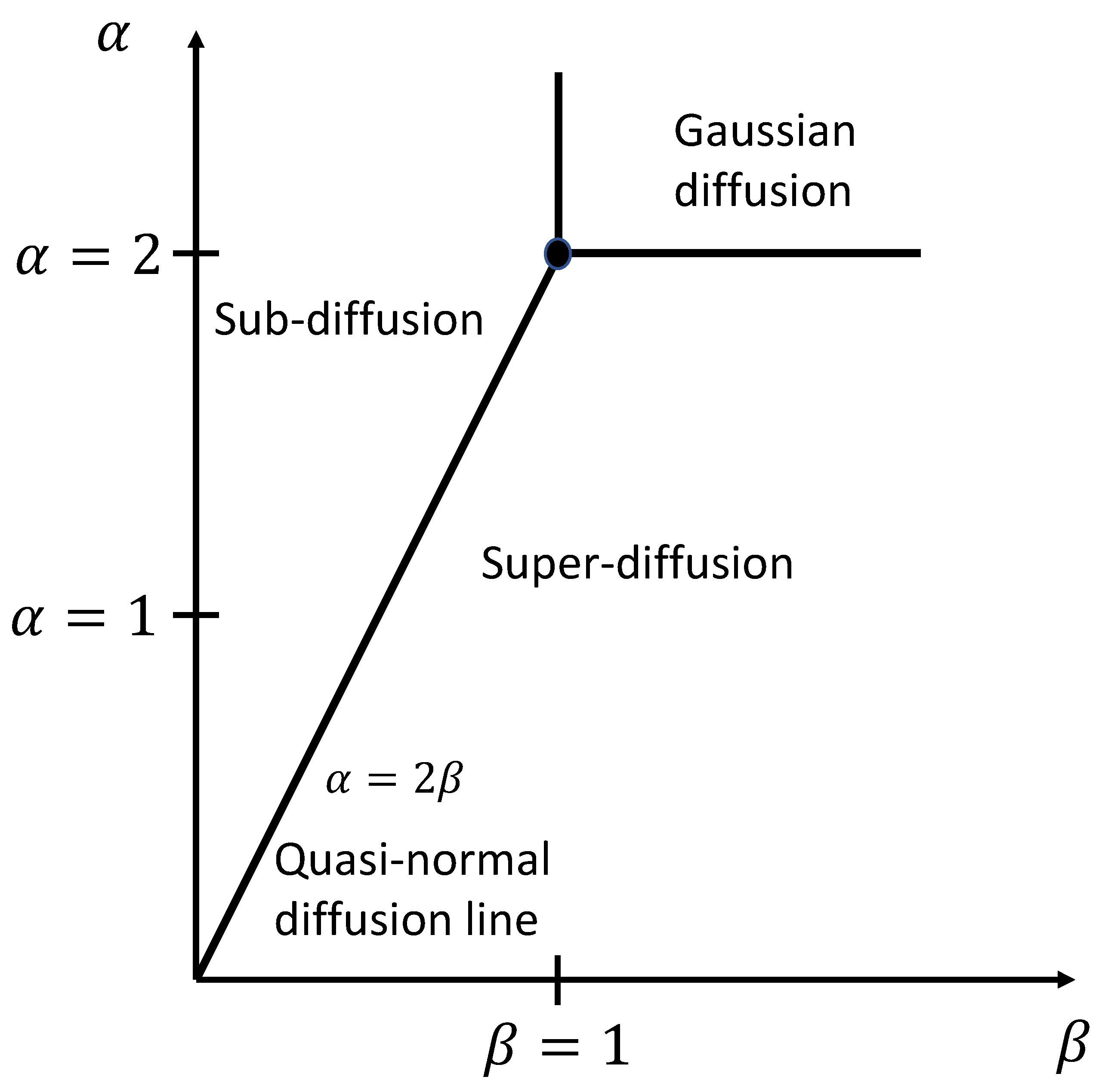
Here when $0<\beta <1$, and $0<\alpha <1$, the equation has solutions for the initial value problem of free particle diffusion under Cauchy boundary conditions that are expressed in terms of the Fox H-functions [33]. Graphically, the domain of these solutions is displayed as an anomalous diffusion phase diagram $\left\{\beta ,\alpha \right\}$—see Figure 2—in which the Gaussian solution corresponds to the point, $\left\{\beta =1,\alpha =2\right\}$, and the mean squared displacement falls on the line, $\left\{\alpha =2\beta \right\}$; hence $〈x^2〉=2D_{\beta ,\alpha }{t}^{2\beta /\alpha }$, where $D_{\beta ,\alpha }$ has the units $m^{\alpha }/s^{\beta }$. The right triangle above this line, and bounded by lines, $\beta =0,\alpha =2$ corresponds to sub-diffusion $\left(2\beta /\alpha <1\right)$, while the right triangle below this line, and bounded by the lines, $\beta =1,\alpha =0$, corresponds to super-diffusion $(2\beta /\alpha >1)$. The line, $\alpha =2$, for $0<\beta <1$ describes subordinated Brownian motion with Mittag–Leffler function solutions, while the line $\beta =1,0<\alpha <2$, corresponds to Lévy motion with stretched exponential solutions [34]. The phase diagram region above $\alpha =2$, for $0<\beta <1$ is one of ultraslow diffusion, while the region to the right of $\beta =1,0<\alpha <2$ displays hyper-diffusion (with a ballistic motion when $\alpha =\beta =2$). The entire region of the anomalous diffusion phase diagram above and to the right of the lines $\beta =1,\alpha =2$ is one of Gaussian diffusion. This is a consequence of taking the limit as the spatial and complex frequencies go to zero in the Fourier–Laplace domain when deriving the anomalous diffusion equation for the continuous time random walk model [35].

In the same way that fractional calculus extends the Gaussian model of diffusion, fractional calculus could be used to broaden the governing equations of statistical mechanics (e.g., Boltzmann, Fokker–Planck, Langevin) to account for memory in time-dependent events and non-locality in physical processes [36]. Before we consider this larger realm of statistical mechanical models, in the next section we will briefly review how fractional calculus can be used to generalize the kinetic theory of gases using the van der Waals model of a gas as an example.

3. Kinetic Theory and Equations of State

The kinetic theory of gases uses classical mechanics to derive equations that predict the equilibrium and non-equilibrium (transport) behavior of gases and liquids observed in the laboratory [37]. Hence, the physical chemistry of simple fluids proceeds from estimates of the molecular velocity, collision frequency, and mean free path to macroscopic averages expressed in terms of the pressure, volume, temperature $\left\{P,V,T\right\}$, number of moles $\left\{n\right\}$, and density $\left\{\rho =n/V\right\}$ or its reciprocal, the molar volume, $\{\overline{V}=V/n\}.$ The resulting statistical averages are manifest as equations of state, beginning with the non-interacting, point masses of the idea gas law, $PV=nRT$, (R is the universal gas constant), and proceeding to the van der Waals equation, which introduces correction terms for molecular size and attractive/repulsive intermolecular forces.

Van der Waals is well-known for his equation of state, which provides a first order model of a real gas [38]. It can be written as:

$$\begin{array}{c}\hfill \left(P+\frac{a{n}^2}{V^2}\right)\left(V-bn\right)=nRT,\end{array}$$

(6)

where the constant b subtracts the finite radius of gas molecules from total volume, and the constant a accounts for the weak “attraction” between neutral gas molecules. The values of b and a are determined from experimental measurements and tabulated for each gas. Van der Waals equation reduces to the ideal gas law $PV=nRT$ at high temperatures and low densities and exhibits an inflection (critical) point that predicts the liquid–gas condensation observed in the two-phase region of pressure-volume plots and on pressure–temperature phase diagrams [39]. It is worth mentioning that extensions of the state equations have been investigated in the context of fractional calculus by extending the thermodynamics relations [40,41,42] or by considering a generalized thermostatistics context associated to a different entropic form [43,44].

Van der Waals is perhaps less well-known for the “correspondence” principle, a proposal he made that since gases exhibit common physical properties (e.g., triple point, critical point, Boyle isotherm, etc.), they should be described by a common reduced equation of state [25] when the pressure, temperature, and specific volume are normalized using the critical point $\left(P_c,{\overline{V}}_c,T_c\right)$—where the gas and liquid phases are indistinguishable:

$$\begin{array}{c}\hfill P_r\equiv \frac{P}{P_c},T_r\equiv \frac{T}{T_c},{\overline{V}}_r\equiv \frac{\overline{V}}{{\overline{V}}_c}.\end{array}$$

(7)

where $\overline{V}$ is the specific volume of the gas (i.e., the reciprocal of gas density, with units (m${}^3$/gram or m${}^3$/mole), so that the reduced van der Waals equation of state, $f(P_r,{\overline{V}}_r,T_r)=0$, can be written as:

$$\begin{array}{c}\hfill \left(P_r+\frac{3}{{\overline{V_r}}^2}\right)\left({3\overline{V}}_r-1\right)=8T_r.\end{array}$$

(8)

In addition, at the critical point the a and b constants in the van der Waals equation and the compressibility factor, $z=P\overline{V}/RT$ can be expressed in terms of $\left(P_c,{\overline{V}}_c,T_c\right)$, as:

$$\begin{array}{c}\hfill a=\frac{27}{64}\frac{R^2{T_c}^2}{P_c},b=\frac{1}{8}\frac{R{T}_c}{P_c},z_c=\frac{P_c{\overline{V}}_c}{R{T}_c}=\frac{3}{8}.\end{array}$$

(9)

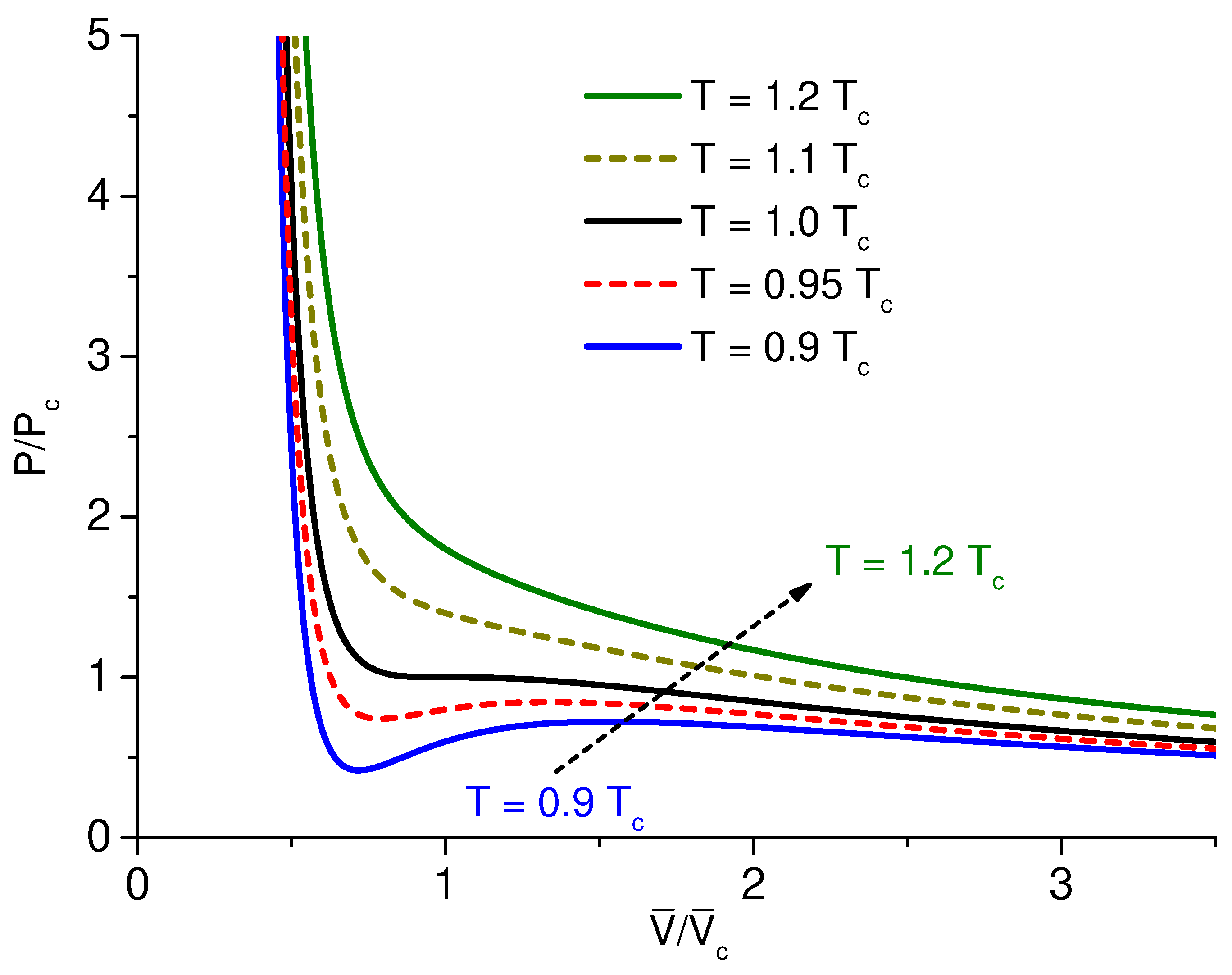
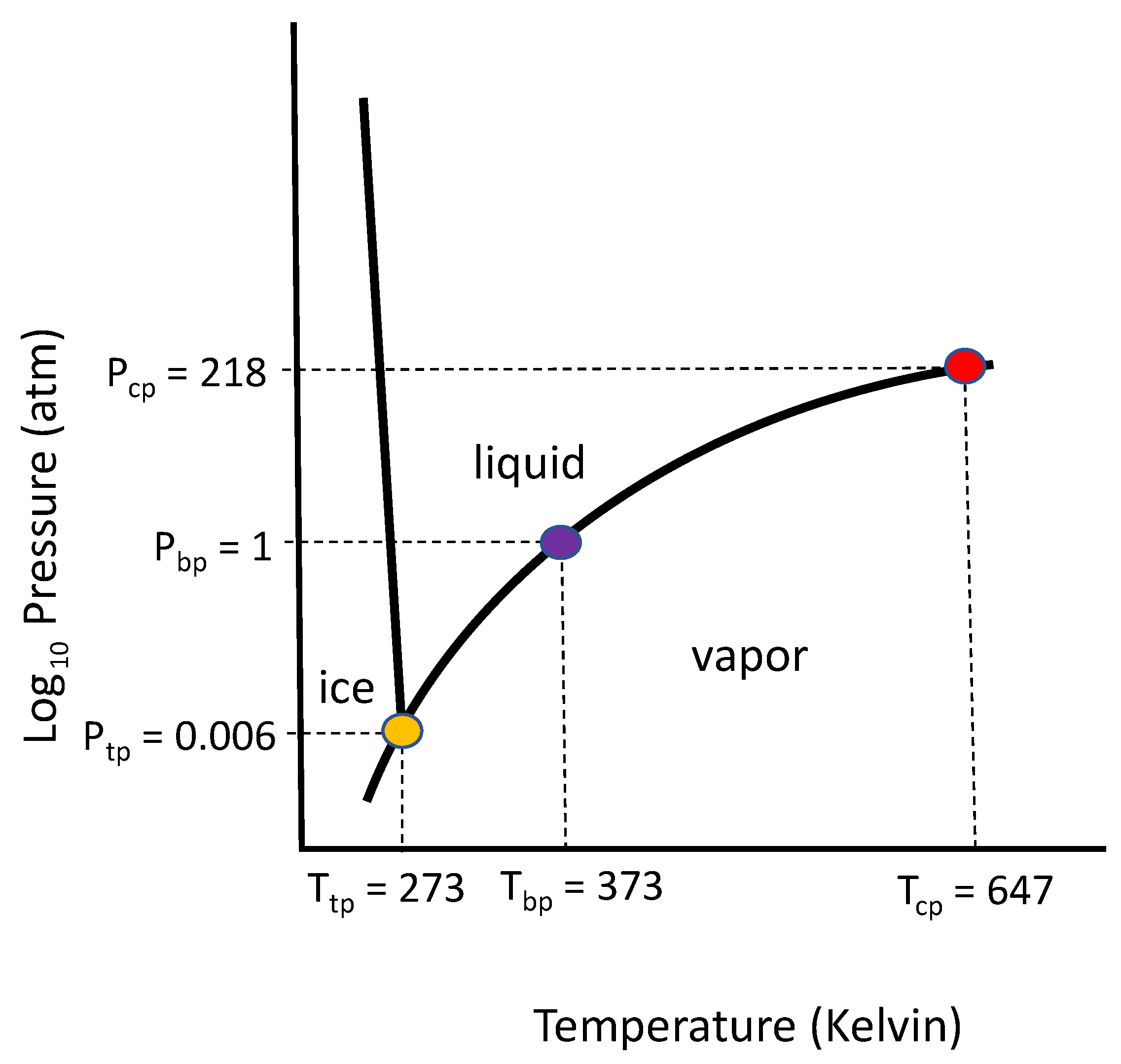
The behavior of a mole of a van der Waals gas is typically described [45] by a plot of $\left\{P,\overline{V}\right\}$ at different temperatures, as an example, see Figure 3. In the region above the critical point $\left\{P_c,{\overline{V}}_c,T_c\right\}$, there is a single-phase region where the gas and liquid coalesce and are indistinguishable (equal densities) and below the critical point by the two-phase region where the liquid and gas phases coexist. Another way to display the behavior of a van der Waals gas is a $\{P,T\}$ plot. As an example, the solid–liquid–gas phase behavior for a fixed specific volume of water (H${}_2$O) is described by a $\left\{P,T\right\}$ phase diagram, Figure 4 [46].

In Figure 4, the vaporization curve ends at the critical point, but along the curve, the slope as a function of temperature is determined by the Clausius–Clapeyron equation [38], which is written below in terms of the specific volume $\overline{V}$ and specific entropy $\overline{S}=S/n$:

$$\begin{array}{c}\hfill \frac{dP\left(T\right)}{dT}=\frac{{\overline{S}}_{gas}-{\overline{S}}_{liquid}}{{\overline{V}}_{gas}-{\overline{V}}_{liquid}}.\end{array}$$

(10)

Hence, the specific volume and specific entropy are related to the specific enthalpy by the partial derivatives:

$$\begin{array}{c}\hfill \overline{V}\left(P,T\right)={\left.\frac{\partial \overline{G}}{\partial P}\right|}_T,and\overline{S}\left(P,T\right)=-{\left.\frac{\partial \overline{G}}{\partial T}\right|}_P.\end{array}$$

(11)

For a van der Waals gas, the specific enthalpy $\overline{G}=G/n$ is given by (see Ref. [20], Chapter XI):

$$\begin{array}{c}\hfill \overline{G}\left(P,\overline{V},T,\right)=P\overline{V}-\frac{3}{2}RTlnT-RTln\left(\overline{V}-b\right)-\frac{a}{\overline{V}}-RT{f}_0,\end{array}$$

(12)

where R is the ideal gas constant, a and b are the van der Waals constants for water, and $f_0$ is a normalization constant.

The phase behavior displayed in Figure 4 is consistent with the Gibbs phase rule (see Ref. [38], pp. 264–269), and similar $\left\{V,T\right\}$ and $\left\{P,T\right\}$ plots are displayed by many substances. In

Table 1. Normalized thermodynamic properties of simple gases at standard temperature (273.15 K) and pressure (1 atmosphere).

Gas	Boiling Point ${\mathit{T}}_{\mathit{bc}}/{\mathit{T}}_{\mathit{c}}$	Boyle’s Temperature ${\mathit{T}}_{\mathit{c}}/{\mathit{T}}_{{\mathit{Boyle}}^{\prime }\mathbf{s}}$	Compression Factor ${\mathit{P}}_{\mathit{c}}{\overline{\mathit{V}}}_{\mathit{c}}/\left({\mathit{RT}}_{\mathit{c}}\right)$
$Ne$	0.607	0.293	0.296
$Ar$	0.576	0.298	0.291
$Xe$	0.566	0.289	0.290
$O_2$	0.585	0.296	0.292
$N_2$	0.611	0.296	0.291
$C{O}_2$	0.641	0.297	0.274
$CO$	0.613	0.292	0.294
$C{H}_4$	0.581	0.298	0.290
$S{O}_2$	0.613	0.297	0.269
$H_{2}O$	0.576	0.297	0.230
Kinetic Theory	∼0.6	0.375	0.375

, for example, we list the properties of a few common gases to show the concordance of behavior (boiling point, Boyle’s temperature, and compression factor) when each gas is normalized to its critical point. The Boyle’s temperature—approximately three times the critical temperature—indicates the $\left\{V,T\right\}$ regime of ideal gas law behavior where the compression factor, $z=P\overline{V}/RT=1$, while van der Waals model predicts, $z=3/8=0.375$ and $T_{Boyle}/T_c=a/bR$ (see Ref. [47], pp. 119–120). Boyle’s temperature also corresponds to the temperature where the slope of the compression factor curve $dz/d{P}_r=0$ and where the second virial coefficient, $B^{\prime }\left(T\right)=\{\left(b-\left(a/RT\right)\right\}/RT$—obtained from a power series expansion of the reduced form of van der Waals equation—is equal to zero (see Ref. [24], pp. 168–169):

$$\begin{array}{c}\hfill z=\frac{P_r{\overline{V}}_r}{R{T}_r}=\left(1+B^{\prime }{P}_r+C^{\prime }{P_r}^2+D^{\prime }{P_r}^3+\cdots \right).\end{array}$$

(13)

In this table, $T_b$ is the boiling point temperature (at 1 atm), $T_{Boyle}$ is Boyle’s temperature, $T_c$ is the critical temperature, $P_c$ is the critical pressure, $\overline{V_c}$ is the critical specific volume (mL/mol), and R is the universal gas constant (8.314 kJoules/kg·mole·K).

The value for the compression factor predicted by the van der Waals gas model (0.375 when normalized to the critical point) is larger than that observed for the real gases listed in Table 1, as might be expected for this simple equation of state. Nevertheless, the data—except for the polar water molecule—are quite consistent (0.27–0.29) with each other. In addition, for the simple gases listed in Table 1, the normalized Boyle’s temperature, boiling point (∼0.6), and critical pressure are all similar. This behavior reflects the regularity of simple gases when described by a “reduced” van der Waals equation, at least in the regions above and below the critical point (see Ref. [24], pp. 165–166). In fact, the compression factor, z, balances the competing influences of attractive ($z<1$) and repulsive ($z>1$) forces, which are separated by the case of $z=1$ for an ideal gas (Figure 10.3 in Ref. [24] p. 166).

Overall, the data illustrate that the fundamental assumptions of the classical kinetic theory are justified for inert, diatomic, non-polar, and some polar gases [48]. Specifically, the simple kinetic theory of gases assumes: (i) the temperature fixes the mean velocity, (ii) the diameter of molecules is small compared with the distance between collisions (mean free path), and (iii) while the frequency of collisions is high, only binary collisions (with no velocity correlation) need to be considered. Advanced models using hard sphere models for molecules and calculations that account for the persistence of velocity in collisions bring closer agreement, at least for conditions near standard laboratory conditions [49]. The extreme conditions of high density and very low temperatures require statistical mechanics and quantum mechanical calculations of the molecular properties [50].

Statistical mechanics provides a natural way to extend the two-parameter empirical equations of state (van der Waals, Dieterici, Berthelot, etc; see Ref. [1], p. 47, Table 1.4) to account for memory in time-dependent events, correlation of momentum before and after collisions, as well as introducing non-locality in transport processes [51]. The Boltzmann equation, for example, directly connects the effects of random collisions and an assumed molecular interaction potential, $V\left(r\right)$, (inverse power law) or the attractive/repulsive two-term Lennard–Jones molecular potential by calculating a molecular collision integral. The statistical moments of the resulting distribution function can be used to determine each coefficient of the virial expansion (see Ref. [52], pp. 231–233). For example, for the second virial coefficient as a function of temperature and the intermolecular potential, $V\left(r\right)$ (see Ref. [48], pp. 225–230) is:

$$\begin{array}{c}\hfill B^{\prime }\left(T\right)=\frac{B\left(T\right)}{kT}=2\pi {\int }_0^{\infty }\left(1-e^{-V\left(r\right)/kT}\right)r^{2}dr.\end{array}$$

(14)

Here r is the radial separation distance between molecules, and k is the Boltzmann constant.

Fractional calculus provides an alternative way to generalize each term of the Boltzmann, Fokker–Planck, and Langevin equations. In the case of the virial equation, one could use the fractional version of Taylor’s theorem:

$$\begin{array}{c}\hfill z_F=\frac{P_r{\overline{V}}_r}{R{T}_r}=\left(1+B_F^{\prime }{P}_r^{\gamma }+C_F^{\prime }{P}_r^{1+\gamma }+D_F^{\prime }{P}_r^{2+\gamma }+\cdots \right),\end{array}$$

(15)

where the fractional virial coefficients $B_F^{\prime },C_F^{\prime },$ and $D_F^{\prime }$ involve fractional derivatives of fractional order, $\gamma$ (see Ref. [53], pp. 88–89 and Ref. [54], p. 54). Likewise, near the critical point, Hilfer has derived a fractional calculus version of the Clausius–Clapeyron equation that justifies the fractional order divergence of the change in specific entropy. Additional examples of how fractional calculus can—and has been—used to extend kinetic theory will be described in the following sections.

4. Kinetic Theory and Transport Theory

In the 19th and 20th centuries, kinetic theory established the existence of atoms in physics and demolished the need for caloric fluid in chemistry. During this, time contributions by Maxwell, Bernoulli, Boltzmann, Clausius, Gibbs, Einstein, Smoluchowski, Jeans, Sutherland, and Loschmidt were at the forefront of theoretical physics. Today, kinetic theory is supplanted by statistical mechanics and quantum mechanics; nevertheless—revised and updated—kinetic theory remains valid for calculating the macroscopic properties of gases [50]. For example, the heat capacity, compressibility, and expansion coefficient as a function of temperature and pressure can be predicted with an accuracy sufficient for engineering and industrial applications [49].

Kinetic theory can also be applied in non-equilibrium situations where liquids and gases carry heat, momentum, and mass. Specifically, when gradients in temperature, velocity, or mass are introduced, kinetic theory predicts the observed transport in terms of the corresponding flux (quantity per unit area, per unit time) via the coefficients of thermal conductivity, $\kappa$, viscosity, $\eta$, and diffusion, D [37]. Typical expressions for the thermal conductivity, $\kappa$, viscosity, $\eta$, and diffusion, D, are displayed in

Table 2. Formulas for thermal conductivity, $\kappa$, viscosity, $\eta$, and diffusion, D, showing representation in terms of kinetic theory ($\rho$, $\overline{v}$, $\lambda$, and $c_v$) and thermodynamic variables (P,V,T) [49].

Transport Coefficient	Property Transported	Kinetic Theory	Units (cgs)
Viscosity, $\eta$	Momentum, $\left(mv\right)$	$\eta =\frac{1}{2}\rho \overline{v}\lambda$	$\frac{g}{cm·sec}$
Thermal Conductivity, $\kappa$	Energy, $\left(\frac{1}{2}m{v}^2\right)$	$\kappa =\frac{1}{3}\rho \overline{v}{c}_v$	$\frac{erg}{cm·sec·deg}$
Diffusion, D	Mass, $\left(m\right)$	$D=\frac{1}{3}\overline{v}\lambda$	$\frac{c{m}^2}{sec}$

.

These formulas connect the microscopic behavior of molecules (particles per unit volume, mean velocity, collision frequency, and mean free path) with the macroscopic thermodynamic properties of the system (temperature, pressure, and specific volume).

Despite the simplicity of the models, they account for the qualitative $\left(T,P,\overline{V}\right)$ behavior of simple gases to within an order of magnitude of the experimental values, and statistical mechanics provides techniques to close that gap (see Ref. [55], Chapter 17 and Ref. [56]). In addition, Zwanzig [36] has outlined extensions of kinetic theory to account for memory in molecular collisions and non-locality in transport (convection and streaming) by using time or space convolutions in generalized versions of the Master, Boltzmann, Langevin, and Fokker–Planck equations.

A direct link between the equilibrium equation of state and the non-equilibrium transport equations is provided by the Langevin equation [57]. This classical description of Brownian motion, pioneered by Einstein, Sutherland, and Smoluchowski [58], establishes a connection between molecular motion and statistical fluctuations. The corresponding stochastic process was simply described by Langevin as:

$$\begin{array}{c}\hfill m\dot{v}\left(t\right)=-\gamma mv\left(t\right)+F\left(t\right)+R\left(t\right).\end{array}$$

(16)

Here m is the particle’s mass, $\dot{v}\left(t\right)$ is the first order, time derivative of the particle velocity, $\gamma$ is the frictional drag coefficient, $F\left(t\right)$ is an applied time-varying force, and $R\left(t\right)$, is a random force obeying the conditions:

$$\begin{array}{c}\hfill 〈R\left(t\right)〉=0;〈v\left(t\right)R\left(t\right)〉=0,\end{array}$$

(17)

which summarizes the assumptions that the ensemble average of random force is zero and that $R\left(t\right)$ is not correlated with the particle velocity. Under these restrictions [58], when $F\left(t\right)=0,$ the velocity autocorrelation coefficient$,〈v\left(t\right)v\left(t^{\prime }\right)〉$ at equilibrium is:

$$\begin{array}{c}\hfill 〈v\left(t\right)v\left(t^{\prime }\right)〉=\left(kT/m\right)exp\left[-\gamma \left|t-t^{\prime }\right|\right].\end{array}$$

(18)

The Langevin equation, which assumes that the drag term depends on instantaneous velocity, can also be extended to include the memory of past behavior by generalizing the drag constant, $\gamma =kT/D$, through a time-dependent, memory function, $\gamma \left(t\right)$ [36], which is incorporated into the Langevin equation by convolution:

$$\begin{array}{c}\hfill m\dot{v}\left(t\right)=-m{\int }_0^t\gamma (t-t^{\prime })v\left(t^{\prime }\right)dt+R\left(t\right)+F\left(t\right).\end{array}$$

(19)

Then, for the simple case of an inverse power-law memory function, $\gamma \left(t\right)={{\gamma }_{\alpha }t}^{\beta -1}$, we obtain an expression for the Riemann–Liouville fractional integral, ${{}_0^{RL}D}_t^{\beta -1}v\left(t\right)$, and the following mixed order differential equation (see Ref. [16], Chapter 12):

$$m\dot{v}\left(t\right)=-m\mathsf{\Gamma }\left(\alpha \right){{}_0^{RL}D}_t^{\beta -1}\left[v\left(t\right)\right]+R\left(t\right)+F\left(t\right).$$

The solution to this mixed order differential equation [22] with $0\le \beta \le 1$ is a single-parameter Mittag–Leffler function, such that when $F\left(t\right)=0,$ the velocity autocorrelation coefficient is:

$$\begin{array}{c}\hfill 〈v\left(t\right)v\left(t^{\prime }\right)〉=\left(2kT/{\gamma }_{\alpha }m\right)E_{2-\alpha }\left[-{\gamma }_{\alpha }{\left|t-t^{\prime }\right|}^{2-\beta }\right].\end{array}$$

(20)

This expression for the velocity autocorrelation coefficient collapses to the exponential function when $\beta =1$ decays as a stretched exponential,

$$\begin{array}{c}\hfill 〈v\left(t\right)v\left(t^{\prime }\right)〉\sim exp\left[-{\gamma }_{\alpha }{\left|t-t^{\prime }\right|}^{2-\beta }/\mathsf{\Gamma }(3-\beta )\right],\end{array}$$

(21)

for short times and behaves as an inverse power-law function,

$$\begin{array}{c}\hfill 〈v\left(t\right)v\left(t^{\prime }\right)〉\sim {{\gamma }_{\alpha }\left|t-t^{\prime }\right|}^{2-\beta }/\mathsf{\Gamma }(\beta -1),\end{array}$$

(22)

for large values of the time. The mean squared displacement for this model [59] for long times is:

$$\begin{array}{c}\hfill 〈\Delta x^2\left(t\right)〉\cong \frac{2kT}{{\gamma }_{\beta }m}\frac{t^{\beta }}{\mathsf{\Gamma }\left(1+\beta \right)},\end{array}$$

(23)

which exhibits sub-diffusion for $\beta <1$ and super-diffusion for $\beta >1$. Notice that the free energy and entropy functions can be evaluated from Equation (19) as worked out in Ref. [60], resulting in a fractional power-law decay for the entropy.

The fractional Langevin equation has been employed to describe the condensed phase behavior of liquids [61], macromolecules in the cytoplasm of cells [62], and electron donor and accepter exchange between fluorescein and anti-fluorescein [63].

Extending the Langevin equation, the Fokker–Planck equation [64] provides a more complete stochastic model of the time evolution of the particle distribution, $P(x,t)$, one that includes both particle velocity, $v\left(x,t\right)$, and diffusion, $D\left(x,t\right)$ (see Ref. [28], pp. 271–220):

$$\begin{array}{c}\hfill \frac{\partial P(x,t)}{\partial t}=\frac{{\partial }^2}{\partial x^2}\left(D\left(x,t\right)P\left(x,t\right)\right)-\frac{\partial }{\partial x}\left(v\left(x,t\right)P\left(x,t\right)\right).\end{array}$$

(24)

Also known as the advection–diffusion equation, it can include external forces and fields [34,65]. The Fokker–Planck equation has a natural generalization using fractional calculus for constant values for velocity and diffusion coefficient [29] as:

$$\begin{array}{c}\hfill {{}_0^{C}D}_t^{\beta }\left\{P\left(x,t\right)\right\}=D_{\beta ,\alpha }\left\{\frac{{\partial }^{\alpha +1}P\left(x,t\right)}{\partial {\left|x\right|}^{\alpha +1}}\right\}-v_{\beta ,\alpha }\left\{\frac{{\partial }^{\alpha }P\left(x,t\right)}{\partial {\left|x\right|}^{\alpha }}\right\}.\end{array}$$

(25)

when $0<\beta <1$ and $0<\alpha <1$.

This fractional calculus version of the Fokker–Planck equation includes memory and nonlocality in the underlying model of the advection–diffusion equation. Going beyond these empirical models of mass, momentum, and energy transport will require looking deeper into the phase behavior of gases and liquids and introducing the Boltzmann and the fractional Boltzmann equations. Notice that these approaches can also be connected to a random walk, with a suitable choice for the probability density function. The scaling of the walks can also be related to the critical phenomena, as discussed in Ref. [66], introducing another possibility for analyzing systems near the phase transition.

5. Kinetic Theory and Transport Coefficients

The transport coefficients derived using kinetic theory (thermal conductivity, viscosity, and diffusion [48] can be partitioned in unitless combinations (e.g., Prandtl and Schmidt numbers (see Ref. [67], p. 16, Table 1.2–3)) that form a basis for comparing families of molecules (polar/non-polar, monoatomic/diatomic, linear/non-linear, symmetric/asymmetric, etc.). For example, in heat transfer, the Prandtl number (momentum/energy) expresses the diffusivity ratio that balances heat transfer due to fluid motion and thermal diffusion, while in mass transfer the Schmidt number (momentum/mass) expresses the diffusivity ratio that expresses the trade-off between mass transfer in the hydrodynamic boundary layer versus the concentration gradient boundary layer (see Ref. [4], pp. 223–228). Because of the equipartition of energy (translation, rotation, vibration), the Prandtl number predicted by kinetic theory for translation alone (3/2) decreases for molecules with additional degrees of freedom, such as the sequence: He, H${}_2$, O${}_2$, CO, CO${}_2$, H${}_2$O, CH${}_4$, C${}_2$H${}_6$, and C${}_3$H${}_8$. Clearly, the transport coefficient values predicted by basic kinetic theory do not match experimental measurements—that require quantum and statistical mechanics—but for data collected near room temperature and atmospheric pressure, simple kinetic theory gives values that are consistent for similar groups of molecules. This concordance is also evident for the Prandtl and Schmidt numbers (and the ratios of specific heats) for the gases listed in

Table 3. Dimensionless ratios of thermodynamic quantities for simple gases.

Gas	Specific Heat Ratio $\frac{{\mathit{c}}_{\mathit{p}}}{{\mathit{c}}_{\mathit{v}}}$	Schmidt’s Number $\frac{\mathit{\rho }\mathit{D}}{\mathit{\eta }}$	Prandtl’s Number $\frac{\mathit{\kappa }}{\mathit{\eta }{\overline{\mathit{c}}}_{\mathit{P}}}$	PT-Ratio $\frac{{\mathit{log}}_{\mathbf{10}}\left({\mathit{P}}_{\mathit{c}}/{\mathit{P}}_{\mathit{tp}}\right)}{\mathbf{2}\left({\mathit{T}}_{\mathit{c}}-{\mathit{T}}_{\mathit{tp}}\right)/{\mathit{T}}_{\mathit{tp}}}$
$Ne$	1.67	1.36	1.51	1.10
$Ar$	1.67	1.33	1.49	1.20
$Xe$	1.65	1.33	1.56	1.16
$O_2$	1.40	1.33	1.39	1.23
$N_2$	1.40	1.34	1.40	2.44
$C{O}_2$	1.28	1.38	1.28	1.42
$CO$	1.40	1.43	1.36	1.24
$C{H}_4$	1.32	1.42	1.34	1.18
$S{O}_2$	1.29	1.25	1.16	1.56
$H_{2}O$	1.33	2.52	0.99	1.66
Kinetic Theory	1.5	1.2	1.5

.

In Table 3, the PT-ratio:

$$\begin{array}{c}\hfill \frac{lo{g}_{10}\left(P_c/P_{tp}\right)}{2({(T}_c-T_{tp})/T_{tp})}\end{array}$$

(26)

is also displayed for each gas. This ratio emerges from applying the Clausius–Clapeyron equation to the liquid–gas vaporization curve (see Ref. [39], pp. 193–196) in the form:

$$\begin{array}{c}\hfill \frac{dP}{dT}=\frac{H_{lg}}{T({\overline{V}}_g-{\overline{V}}_l)}=\frac{{PH}_{lg}}{R{T}^2},\end{array}$$

(27)

where $H_{lg}$, is the heat of vaporization. Assuming a mole of an ideal gas with ${\overline{V}}_l\ll {\overline{V}}_g$, integration yields $2.303{log}_{10}\left(P\right)={C_o-H}_{fg}/RT$, (see Ref. [38], pp. 248–250) where $C_o$ is a constant of integration, hence two points $\left\{P_1,T_1\right\}$, $\left\{P_2,T_2\right\}$ on the vaporization curve:

$$\begin{array}{c}\hfill {log}_{10}\left(\frac{P_2}{P_1}\right)=\frac{H_{lg}}{2.303R{T}_2}\left(\frac{T_2-T_1}{T_1}\right).\end{array}$$

(28)

In applying the first order liquid–gas phase transition characterized by the Clausius–Clapeyron equation to the gases in Table 3, we are assuming that this simple model applies for a van der Waal gas in the $\left\{P,T\right\}$plane from the triple point $\left\{P_{tp},T_{tp}\right\}$, through the boiling point $\left\{1atm,T_{bp}\right\}$ to the critical point $\left\{P_c,T_c\right\}$.

As the temperature approaches the critical temperature, the slope of the Clausius–Clapeyron equation diverges (${\overline{V}}_{gas}\approx {\overline{V}}_{liquid})$, and we must use the Ehrenfest equation [2] to fit the jump discontinuity:

$$\begin{array}{c}\hfill \frac{dP\left(T\right)}{dT}=\frac{c_{P,gas}-c_{P,liquid}}{T_c{\overline{V}}_c\left({\alpha }_{P,gas}-{\alpha }_{P,liquid}\right)},\end{array}$$

(29)

where $c_P$ is the specific heat at constant pressure, and ${\alpha }_P$ is the isobaric coefficient of thermal expansion. Nevertheless, assuming $\overline{V}=P/R{T}^2$, we find the same logarithmic pressure versus temperature behavior for simple gases.

Finally, both experimental and theoretical results indicate that the relative specific enthalpy diverges as the critical point is approached [68]. Hence, we have:

$$\begin{array}{c}\hfill \overline{G}\left(P\right)-\overline{G}\left(P_c\right)\sim {\left|P-P_c\right|}^{1+\frac{1}{\delta }},\end{array}$$

(30)

where $\delta$ is the equation of state exponent, which in the classical case ($\delta =1$) gives a quadratic exponent.

Hilfer has proposed a fractional calculus extension of the Ehrenfest equation that interpolates between the classical first and second integer orders $1<\omega <2$ (see Ref. [20], Chapter IX). In this model, he computes the radial fractional derivatives for a transition near the origin of a continuous phase space along a direction, e, at the critical pressure $p_c$:

$$\begin{array}{c}\hfill \underset{r\to 0}{\lim }{D}_{r,0^{+}}^{\omega -1,1}\frac{\partial g}{\partial r}\left(p_c+re\right)=g^{\left(\omega \right)}\left(p_{c}e\right)=0.\end{array}$$

(31)

When applied to a van der Waals gas [20], the result is $\omega =4/3$; hence, the order for the approach to the critical point is given by $\omega =1+\frac{1}{\delta },$with $\delta =3$. This behavior is plotted in Figure 5, which shows the behavior of the fractional derivative (slope of the enthalpy versus normalized temperature near the critical point.

Both integer and fractional order models are consistent with the increase in entropy for the fluid–gas transition [24]

$$\begin{array}{c}\hfill S=k_{B}log\left(W_{lg}\right)=\frac{H_{lg}}{T}.\end{array}$$

(32)

where $k_B$ is Boltzmann’s constant, and $\left(W_{lg}\right)$ represents the ratio of available microstates for the two phases. This corresponds to the temperature-entropy change at constant pressure when the system moves from the liquid phase to the two-phase liquid and vapor (constant temperature, but increasing entropy) state and finally with application of external energy (heat) to the superheated vapor (gas phase). Thus, the change in composition reflects increasing entropy in the thermodynamic sense and an increase in the mean free path of the molecules in the vapor phase (compared with the liquid phase).

6. Kinetic Theory and Fractional Calculus Phase Diagram Equivalence

In this section, we suggest that the fractional order phase transition model Hilfer [20] applied to the liquid–gas vaporization curve can be extended to the adjacent liquid and gas regions. This is accomplished by scaling the similar thermodynamic and anomalous diffusion phase diagrams—linking molecular motility with anomalous diffusion. We use “corresponding state” theory (i.e., the insensitivity of gas dynamics to intramolecular properties) to normalize the liquid–gas segment of the thermodynamic $\left\{P,T\right\}$ phase diagram and overlay the result with the fractional calculus (CTRW) phase diagram for anomalous diffusion (the underlying supposition is that restricted diffusion occurs in liquids, while Lévy flights arise due to mesoscale turbulence in gases).

The fluid nature of the liquid and gas phases delineates the axioms of kinetic theory, which are the basis for the corresponding state theory, that is, the similarity in the dynamic behavior (collision frequency and mean free path) for gases and (density or order/disorder parameter and correlation length) for liquids. Essentially, all one needs is a model for the kinematics of collisions and the intermolecular potential (e.g., Lennard–Jones) to ascertain the transport properties of simple gases (e.g., Chapman–Enskog theory, (see Ref. [50] p. 194)) and simple liquids [61]. We will apply this idea to the phase behavior of one-component systems between the triple point $\left\{P_t,T_t\right\}$ and the critical point $\left\{P_c,T_c\right\}$ of the $\left\{P,T\right\}$ phase diagram.

Normalization of the pressure and temperature will be used to estimate the corresponding values of the fractional time and space derivatives in the anomalous diffusion equation. Since the diffusion coefficient can be simply expressed using kinetic theory in terms of the mean velocity and the mean free path, this provides an indirect connection between microscopic and macroscopic properties [67]. Finally, we assume that the normalized equilibrium behavior of molecules described by the system’s phase diagram (between the triple point and the critical point) aligns with the fractional phase behavior of anomalous diffusion along the vapor pressure curve for each gas.

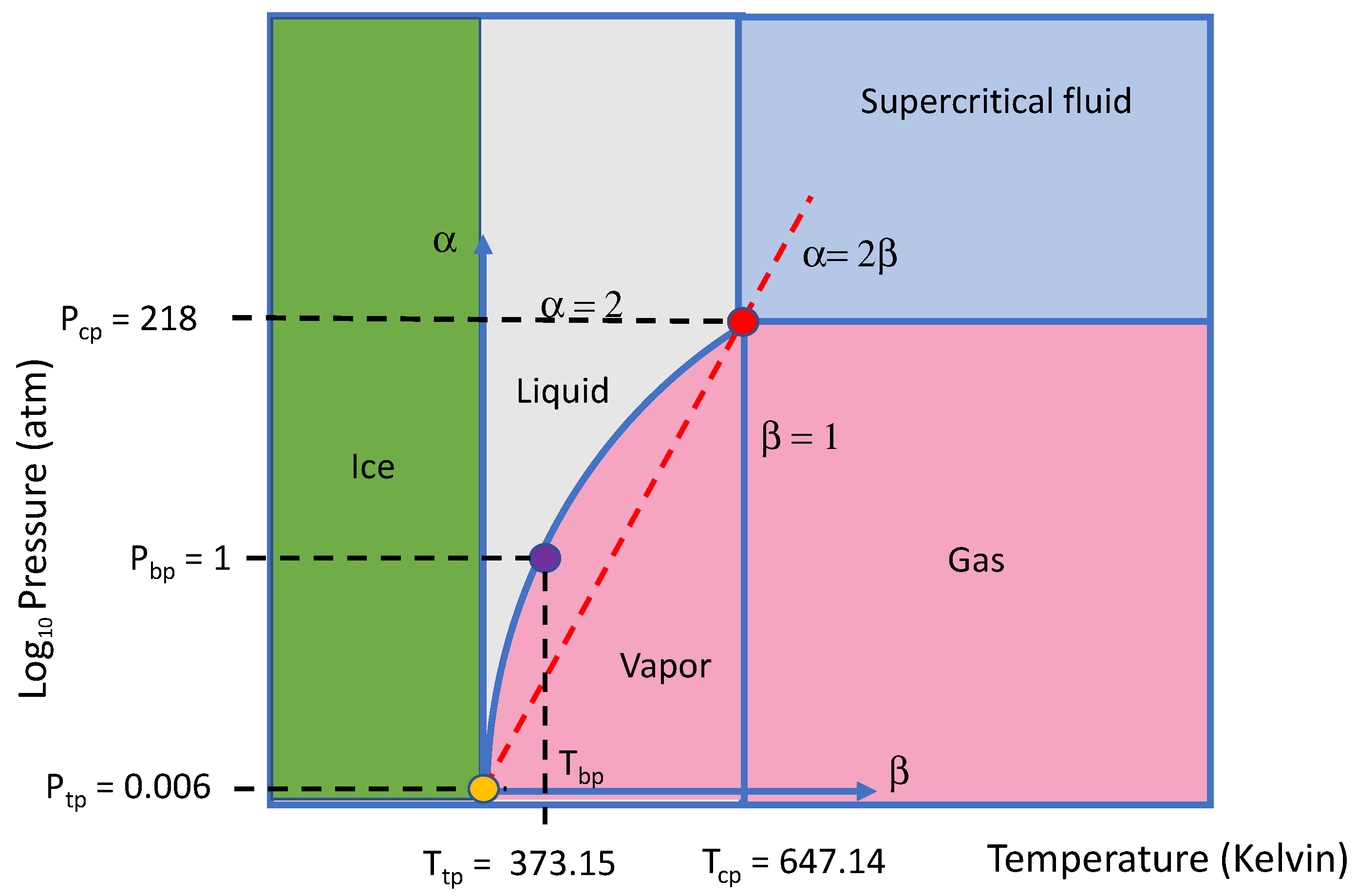
As an example, in Figure 6 we have superimposed a portion of Figure 2 (e.g., the $\{\beta ,\alpha \}$ plane for fractional time and space diffusion with a constant coefficient) onto the phase diagram of pure water, Figure 4 (e.g., from the triple point, tp, to critical point, cp,). Taking inspiration from the Clausius–Clapeyron equation, we normalize the pressure P and temperature T using:

$$\begin{array}{c}\hfill \alpha =2\left[{log}_{10}(P/P_{tp})/{log}_{10}(P_{cp}/P_{tp})\right]\mathrm{and}\beta =\left[\left(T-T_{tp}\right)/\left(T_{cp}-T_{tp}\right)\right]\end{array}$$

(33)

The overlap divides the liquid and vapor phases of water into regions of sub- and super-diffusion, respectively, and suggests that beyond the critical point the supercritical fluid phase corresponds with the domain of Brownian motion in the mathematical phase diagram. This provisional or inchoate connection also appears to be valid for the simple gases listed in Table 1 and Table 3. The idea perhaps could be extended to other situations where anomalous diffusion or behavior appears in porous or fractal materials and for phase transitions close to the percolation threshold. For example, this correspondence might be extended by using fractional calculus for the classification of the critical exponent for liquid crystal, paramagnetic–ferromagnetic, and gel–colloid phase transitions [69,70,71].

7. Discussion

In a previous paper [17], we extended anomalous diffusion phase diagrams (two-dimensional plots $\{\beta ,\alpha \}$ whose axes, $\beta$ and $\alpha$, depict the order of the time and space fractional derivatives, respectively) to a multi-dimensional representation for material exhibiting a power-law behavior described via a time- and space-dependent diffusion coefficient, $D\left(x,t\right)=D_{\upsilon ,\theta }{\left|x\right|}^{\theta }{t}^{\upsilon }$. The goal was to stitch together the four parameters $\{\beta ,\alpha ,\nu ,\theta \}$ on a hypercube frame to illustrate common regions of sub- and super-diffusive phase behavior. In this paper, our aim is to connect the phase behavior of fractional calculus models of anomalous diffusion with the molecular motion occurring near the liquid–vapor phase transitions of simple gases/liquids, behavior first predicted by the kinetic theory of gases and now incorporated into the canon of statistical mechanics.

Our argument (outlined in Figure 1) focuses on the fractional order generalization of the mathematical models of statistical mechanics for gases and liquids under equilibrium and non-equilibrium conditions (i.e., state and transport equations). This investigation cites instances where fractional calculus attributes (memory, non-local and long-range interactions, and inverse power-law decays in the correlation length) are embedded in statistical mechanics. To be specific, we consider the phase behavior of simple gases (neon, argon, xenon, oxygen, nitrogen, carbon dioxide, carbon monoxide, methane, sulfur dioxide, and water) between their respective triple and critical points. In this regime, we rescaled corresponding phase diagrams ($\{T,P\}$ and $\{\beta ,\alpha \}$) to illustrate the natural way fractional calculus can describe the classical physical chemistry: the corresponding Schmidt and Prandtl numbers, the liquid–gas vaporization curves, and the critical exponents for the approach to the critical point.

Fractional calculus interpolates between integer order time and space derivatives so such non-integer order operators can appear in any term of a mathematical model. This generalization provides modeling flexibility but changes the physical picture of dynamic processes, such as molecular collisions and diffusion. Adding to the modeling complexity is the need to select one of the varieties of fractional derivative definitions (see Ref. [31], Chapter 2), the need to employ consistent units to match experimental data, and the need to provide a physical interpretation for each time- and space-derivative. Earlier in this paper, when describing a fractional calculus extension of the virial equation of state, we followed Leszczynski [72], who used the fractional calculus version of Taylor’s theorem to generalize the continuum models of classical fluid mechanics (continuity, momentum, thermal energy) to granular flows. This approach seems to us to be a reasonable way to maintain contact with classical results on one hand and with “anomalous” fluid behavior near phase boundaries on the other hand.

Here, being guided by the Clausius–Clapeyron equation, we have normalized the $\{P,T\}$ phase diagram for water with respect to its triple and critical points and found that analogous regions of gas–liquid–vapor equilibrium correspond with regions of sub- and super-diffusion in the non-equilibrium $\{\beta ,\alpha \}$ phase diagram for anomalous diffusion (Figure 6). Briefly, the line $\beta$ = $\alpha /2$, (along which the mean squared displacement is linear in time) divides the liquid and vapor phases of water into regions of sub- and super-diffusion. Both diffusion domains are bound by a region where the supercritical fluid phase exists. Mathematically, the supercritical domain corresponds to conditions where Brownian motion and Gaussian distributions predominate. Physically, the supercritical phase reflects coalescing of the liquid and gas phases (i.e., the disappearance of the meniscus boundary) in a region where Gaussian statistics and ideal gas law behavior predominate.

This rudimentary connection is consistent with the van der Waals behavior of simple gases (which approaches ideal gas law behavior at high temperatures and pressures) and with the $\{P,T\}$ phase diagrams of the gases listed in Table 1 and Table 3. An extension to other transport coefficients (e.g., rotational diffusion, viscosity, thermal conductivity) as well as to dielectric polarization and electrical conductivity may be possible. In addition, the correspondence has the potential of linking the order of fractional derivative operators to charge and mass transfer in porous and heterogeneous materials where percolation and fractal structure exhibit anomalous conductivity and diffusion [6,16,73].

Alternatively, we can use fractional calculus to generalize the Boltzmann, Kramers, Langevin, and Fokker–Planck equations of statistical mechanics (e.g., see the books by Tarasov [74] and by Uchaikin and Sibatov [75]). Certainly, the kinetic theory concepts of mean free path and the time between collisions fit the ad hoc assumptions in the CTRW stochastic model of inverse power-law particle jumps and waiting times. Unfortunately, the connection between the CTRW model of inverse particle jump ${\left|x\right|}^{-(1+\alpha )}$ and waiting time $t^{-(1+\beta )}$ probabilities is still an open question and unresolved for molecular dynamics and porous material transport properties [6]. Alternatively, we can describe fractional derivatives in terms of a distribution of first order exponential decay processes [15]. Using this approach, Berbean–Santos analyzed luminescence [76] by associating low order fractional derivatives with a broad distribution of relaxation times that condenses to a single relaxation time when the order approaches one. In both situations, by following the fluctuation–dissipation theorem we found links between the time-dependent position and velocity autocorrelation coefficients and the corresponding diffusion coefficient to establish connections with experimental data.

In addition, the complete Lévy description of anomalous diffusion (Feller–Takayasu diamond) represents an asymmetric stable law where $\alpha$is the Lévy index, and $\theta$is a symmetry index. Hence, it could be placed on the floor of the anomalous phase cube to replace the CTRW model. In a similar manner, the fractional/fractal extension of Hamiltonian dynamics on a fractal described by Zaslavsky [28] has the same general form as the CTRW model, but for his model the order of the fractional time and space derivatives are directly connected with a fractal structure in time and distance in the underlying phase space (p, q) of the Hamiltonian system. Another example is the generalized diffusion coefficient $D(x,t)=D{\left|x\right|}^a{t}^b$ discussed by Evangelista and Lenzi which gives rise to anomalous diffusion depicted by stretched Bessel and Mittag–Leffler functions [29]. Finally, the power-law diffusion coefficient model, which can also be described as a stretched Gaussian is equivalent to a time-dependent power-law (in time) diffusion coefficient and hence is equivalent to the Novikov model: $D\left(t\right)=D_0+D_1/t^{\alpha }$ [65,77].

To recapitulate, phase diagrams are used throughout physics and engineering to map the behavior of physical systems (see Review on States of Matter in Ref. [71]). Chemical phase diagrams of single and multiple components (e.g., water, salt–water, lead–tin, iron–iron carbide) depict experimental data (melting, vaporization, sublimation) in regions representing solid, liquid, and gaseous phases as well as exhibiting power-law singularities in the vapor pressure, compressibility, and thermal conductivity when the critical point is approached, which introduces a parallel universe of critical exponents $\left\{{\alpha }^{\prime },{\beta }^{\prime },{\gamma }^{\prime }\right\}$for thermodynamic and statistical relationships (e.g., compressibility, correlation distance, etc.) that appear close to the critical point. Away from the critical point, numerical and Monte Carlo simulation results for the normal (Gaussian) and anomalous (Lévy, fractional Brownian, subordinated, ballistic) diffusion of ideal particles has been investigated. In this paper, we focus on the thermodynamic vaporization curve and mathematical phase diagrams described by the fractional diffusion equation. Bridging these two representations is the goal of our study.

Following this path, we have noted how fractional calculus can be combined with simple kinetic theory and statistical mechanics to describe the transport properties of simple molecules (e.g., inert and diatomic gases); it will be interesting to test this model using experimental data for larger molecules, such as a series of simple hydrocarbons (methane, ethane, propane, butane, etc.). In addition to establishing a concordance between experimental and theoretical predictions, molecular dynamics calculations of the liquid–vapor phase diagram [49], Ising models on multidimensional lattices [78], and numerical models of heat, mass, and momentum transfer [79] can be examined for the emergence of inverse power-law behavior, such as that observed asymptotically in simple models of atomic dynamic models of fluids [61] and in fractional order phase transitions [20].

8. Conclusions

In this paper, we surveyed studies that applied fractional calculus to statistical mechanics and the kinetic theory of gases. Two aspects of our review are noteworthy: first, we provided a framework for classifying fractional models leading to the equilibrium equations of state and to the non-equilibrium transport of energy, momentum, and mass. Second, we identified a way to overlap the fractional order phase diagram for anomalous diffusion with the corresponding thermodynamic phase diagram for simple gases. The framework is important because it provides a pedagogical road map spanning the micro-, meso-, and macro-time and space scales linking atomic physics to continuum models of gases and liquids. The overlap is phenomenological but suggests characteristics of kinetic theory (collision frequency and mean free path) that have direct representation in the continuous time random walk model of diffusion (trapping time and jump increments). A reasonable deduction is that the statistical ideas incorporated in the macroscopic diffusion equation by the fractional time- and space-derivatives provide measures of microporous particle motion and fractal material structure that are observed via sub- and super-diffusion. This conclusion suggests a direction for future research leading to improved models for fitting experimental data and to a greater understanding of the physical and structural basis for fractional kinetics.