1. Introduction
The paper deals with the stability of the problem of rotation of an isolated liquid mass about a fixed axis. Such problems were treated by many outstanding mathematicians. A review of the topic was presented in the book of Appell [
1]. One can find there, for example, the results of Charrueau [
2,
3], who was one of the first to start studying the problem with a capillarity effect at the beginning of the 20th century.
A. M. Lyapunov [
4,
5] analyzed the stability of equilibrium figures for a rotating fluid mass without surface tension by analytical methods. He investigated the second variation of an energy functional considering small perturbations of the boundary of an equilibrium figure. The positiveness of this variation guarantees the stability of the figure because the energy potential possesses a minimum in this case.
The Lyapunov method was generalized for a rotating capillary fluid by one of the authors of this paper in [
6,
7]. We developed this technique for a finite mass of two-phase liquids. We studied the stability problem for two rotating incompressible capillary self-gravitating fluids with an unknown interface and a free surface to be close to the boundaries of two equilibrium figures inserted into each other. The existence of two-phase figures of equilibrium was obtained in [
8]. We adapted the proof of the global maximal regularity of two-fluid problem without rotation ([
9] Ch. 7, 12) to our case. A study of rotating two-phase drop was performed in the Sobolev–Slobodetskiǐ spaces by ourselves in [
10,
11], where an a priori exponential inequality was obtained for a generalized energy. At first, on this basis, the global solvability of a linearized problem was proved. Next, a solution to the non-linear problem was found as the sum of the solution of the linear homogeneous system and that of a problem with small non-linear terms. We use this technique also in the case of the Hölder spaces. We note that the problem in [
10] governs the rotation without mass force and self-gravity of the drop. In the present paper, we take both these forces into account.
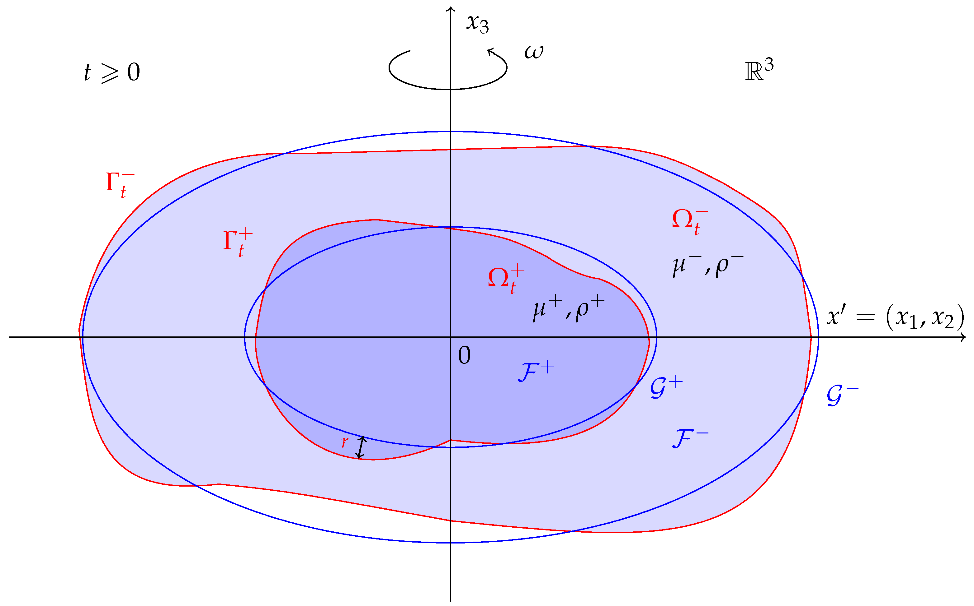
2. Setting of a Problem
We give a mathematical statement of the problem. We assume two immiscible viscous incompressible fluids of densities
and viscosities
to be situated in a domain
which is separated by a variable closed interface
and bounded by a free surface
,
being the boundary of the domain
filled with a fluid of the density
. It is surrounded by another fluid of the density
contained in the domain
(see
Figure 1). At the initial moment
, the boundaries
are given. This two-layer fluid mass rotates about the vertical axis
. One should find the surfaces
, velocity vector field
and pressure function
which satisfy the interface problem for the Navier–Stokes equations:
where
,
,
;
is the vector of mass forces,
is the gravitational constant;
is initial velocity vector field; the stress tensor is
where
is identity matrix,
is the twice rate-of-strain tensor, the superscript
T means the transposition, the step-functions of density and dynamical viscosity
are equal to
in
and
in
, respectively;
are surface tension coefficients on
,
are the doubled mean curvatures of the surfaces
and
at the points where
is convex toward
), the vector
is the outward normal to
and
is the speed of evolution of the surfaces
in the direction of
. A Cartesian coordinate system
is assumed to be introduced in
. The centered dot · denotes the Cartesian scalar product.
The vectors and vector spaces are marked by boldface letters. We imply the summation from 1 to 3 by repeated indices, indicated in Latin letters.
The domains
and
are supposed to be close to equilibrium figures
and
of the same volumes:
In view of the incompressibility of the fluids, equalities (
2) hold for arbitrary
:
Mass conservation follows from the constancy of the densities.
We set
,
and
(see
Figure 1).
If mass force
is orthogonal to all the vectors of rigid motion, i.e.,
a solution of system (
1) also satisfies the additional conservation laws:
where
is the Kronecker delta,
,
is a density step-function:
in
,
in
,
is the angular speed of the rotation and
is angular momentum of the rotating fluids. Under conditions (
4) for
, it was shown in [
8] that laws (
5) are satisfied for all
if they hold at
.
For the new pressure function
, system (
1) transforms into the problem
The uniform rotation of a two-phase drop about the
-axis with constant angular velocity
is governed by the homogeneous steady Navier–Stokes equations:
with the step-function of dynamical viscosity
in
and
in
. The solution of this system is the couple of velocity vector field
and the function of pressure
where
and
and
are step-functions in
. In order to find the equations of the surfaces
of the domains
, we substitute
into boundary conditions (
7)
where
and
are twice the mean curvatures of
and
, respectively, and
In [
8], the existence of the boundaries
satisfying Equation (
8) was proved, provided that
is small enough, and
(Proposition 3.3). It was noted there that
are flattened spheroids. If
, the condition
is not necessary. We cite this proposition.
Proposition 1. Let the angular momentum β be small enough, and and . Then, for given volumes and , there exists a unique equilibrium figure which is axially symmetric about the axis and symmetric about the plane . The surfaces are close to the spheres , respectively, where , are such thatand Thus, we admit the axial symmetry of
and their symmetry about the plane
. Then
Relation (
9) corresponds to the first condition in (
5). It means that mass center of the fluids is in the origin all the time. The other conservation laws in (
5) take the form
Let us consider the perturbations of the velocity and pressure
We introduce the new coordinates
rotating about the
-axis with the angular velocity
and the new unknown functions (
,
) by the formulas
where
We note that
and
By substituting this in (
6) and (
7), acting by
and taking (
8) into account in the boundary conditions, we obtain the following interface problem for the perturbations
and
:
where
,
,
is the outward normal to
,
,
, etc. We note that the kinematic boundary condition
conserves its form (see [
10]).
Relations (
3), (
5) and (
10) go over into
where
.
We give the definition of the anisotropic Hölder spaces which we use below.
Let
be a domain in
,
and
. We set
for
. By
, we denote the set of functions
f in
having the norm
where
and
We introduce the following notation:
Let
. By definition, the space
consists of functions
f with finite norm
where
We define
,
, as the space of functions
,
, with the norm
Here
One also needs the following norm with
:
with
The estimate
is known. By definition,
if
Finally, if a function
f has finite norm
where
we consider that
.
We consider that a vector-valued function belongs to a Hölder space if all of its components belong to this space and define its norm as the maximum of component norms. The same applies to a tensor-valued function.
3. A Linearized Problem
We suppose the surfaces
to be given by the relations
where
is the outward normal to
.
Let us map
into
by the inverse transformation to the Hanzawa transform
where
,
are some extensions of
and
r into
, respectively.
In order to analyze problem (
11) with initial data close to the regime of rotation as a rigid body (see
Figure 1), we linearize it. To this end, we calculate the first variation with respect to
r of the differences
,
,
. We use the following formulas for the first and second variations of a functional
It is easily seen that
By [
12],
where the Laplace–Beltrami operators
act on
. Moreover, as mentioned in [
8],
where
In new coordinates (
15), the kinematic condition for
takes the form
Thus, collecting the above relations, we obtain a linear problem corresponding to (
11) with the unknown functions
and
:
where the operators
with
where
and
are the Gaussian curvatures of
,
is the angular velocity,
is an unknown function equal to the deviation of the surfaces
from
and
are given functions.
First, we study problem (
18) with the homogeneous equations and boundary conditions:
We assume that the domains
are symmetric with respect to
and that the initial data satisfy, due to assumptions (
12), (
13), orthogonality conditions
We put , , , , , .
Proposition 2. A solution of problem (
20)
under conditions (
21)
, (
22)
at the initial instant satisfies (
21)
and (
22)
for all . This proposition is proved in the same way as Proposition 2.1 in [
10] by virtue of Proposition 3.
In view of impulse conservation, the following statement is valid.
Corollary 1. There holds the decompositionwhere means a vector field orthogonal to all the vectors of rigid motion η; i.e., and Proposition 3. The following relations hold:where η is an arbitrary vector of rigid motion. This statement was proved in [
11].
We cite the result obtained in ([
9], § 5.3) about the solvability of the following linear problem for the Stokes system in an unbounded domain
,
, with the closed interface
:
where
f, g, b, b′, B, v0 are given functions;
n denotes the outward unit normal to Γ; II
0a =
a − (
n ·
a)
n.
We assume first that there hold two representations:
and second, that compatibility conditions
are satisfied. The last of relations (
26) follows from the tangential part of the necessary condition of the continuity of velocity derivative
at
. The normal part of this equality
holds if the initial pressure
is a solution to the problem
(Here the first equation is understood in a weak sense.)
Theorem 1. Let assumptions (
25)–(
27)
be fulfilled. In addition, we assume for and when and that , , , , , and the elements of the tensor have finite semi-norms , , We suppose also that all given functions decrease quickly enough for (for example, in a power-law way). Then problem (
24)
has a solution such that , and the inequalityholds, where is a nondecreasing function of T, and is a ball containing the domain . The velocity vector field is defined uniquely, and the pressure p is determined in the class of functions of weak power-law growth up to a smooth bounded time-dependent function. A similar theorem for the bounded domain
is also valid [
9]. In order to prove such a theorem, one applies the estimates near the outer boundary
which were obtained in [
13,
14] for a single liquid.
Theorem 2 (
Local Solvability of the Linear Problem).
Let and with We suppose that and satisfy compatibility conditionswhere Moreover, we assume and to satisfy the representationwhere have finite norm and semi-norm , We also assume the initial pressure to be a solution (in a weak sense) to the problemThen problem (
18)
has a unique solution such that , , for any and the inequalityholds. Proof. Let
be a function satisfying the conditions
and the estimate
Such a
exists. Indeed, we find this function as a solution of a hyperbolic equation with the initial data
and
, where
and
are extensions of the initial data into
with conservation of class. Then
We can write
Hence, problem (
18) can be transformed to the form:
where
,
,
is the surface gradient on
;
. Here we have used (Lemma 10.7 in [
15]) the relation
We can apply Theorem 1, formulated for a bounded domain, to problem (
31) in order to state the solvability of it, the additional terms
and
being of lower order and having no essential influence on the final result. Indeed, let us evaluate, for example, the terms connected with self-gravity:
The others terms can be treated in a similar way. Thus, inequality (
28) together with (
30), (
32) and (
33) implies estimate (
29). □
Let us consider now homogeneous problem (
20) with
and
satisfying orthogonality conditions (
21) and (
22). On the basis of decomposition (
23), an
-estimate of
and
r with exponential weight was obtained in [
11] (Proposition 2.3). We cite it here.
Proposition 4. Assume that the formis positive definite—i.e.,for arbitrary satisfying (
21)
. Then a solution of (
20)–(
22)
is subjected to the inequalitywhere are independent of Remark 1. Condition (
35)
coincides with the positiveness of the second variation of the expression for potential energyfor given volumes of . One can calculate it by (
16)
(see [6,8,11]). Taking into account Equation (
8)
, we finally obtainIf for the subspace of r satisfying orthogonality conditions (
21)
, then the potential is weakly lower semicontinuous. Since is also coercive, it has a minimum which is clear to be realized at . This means the stability of the figures and with the boundaries defined by (
8)
. We note that these relations serve as the Euler equations for . This is variational setting for stability problem of and . Theorem 3 (
Global Existence for the Linear Homogeneous Problem).
We assume that estimate (
35)
is valid for the functional defined by (
34)
and that , , with satisfy orthogonality conditions (
21)
and (
22)
and compatibility oneswith initial pressure function being a solution to the problemThen problem (
20)
has a unique solution such that , , for any , and the inequalityholds with a certain . In order to obtain bounds for the exponentially weighted Hölder norms of a solution, we apply a local-in-time estimate.
Proposition 5. Let . For a solution to problem (
20)–(
22)
, the inequalityis valid, where , , , . Proof of Proposition 5. Let
. We multiply (
20) by the cutoff function
, which is smooth and monotone,
if
and
if
where
In addition, for
and
, the inequalities
hold.
Then, for
,
,
we obtain the system
From Theorem 2 applied to system (
40), (
21) and (
22), it follows that estimate (
29) is valid for
and
, which implies
where
, and
with
; the vector
is extended into the whole
and vanishes at infinity. By Lemmas 1, 2 which are given below, inequality (
41) can be prolonged as follows:
with
, which leads to
Here,
,
.
Setting
, we obtain
This implies
provided that
For
, this inequality coincides with (
39). □
In ([
9] Ch. 5), the following lemma was established on the estimate of Newtonian potential gradient for the Hölder spaces over
.
Lemma 1. If and vanishes at infinity; then, for the gradient of the Newtonian potentialthe inequalitieshold. Interpolation inequalities are proved in a way similar to ([
9] Ch. 6).
Lemma 2. Let with . Then v satisfies the estimateFunctions and are subjected the inequalities Proof of Theorem 3. By Theorem 2 and Proposition 5, one has
Summing (
42) from
to
, we obtain an inequality which implies
By choosing
in (
43) from Proposion 4, we make use of an inequality equivalent to (
36) and add the estimate
Now taking supremum in
, one arrives at (
38). □
4. Global Solvability of the Nonlinear Problem
We separate the normal and tangent parts in the boundary conditions in (
11) after transformation (
15) and take (
17) and (
19) into account. Then this problem can be written in the form ([
9], Ch. 12, [
16]):
where
,
,
,
,
is the Jacobi matrix of transformation (
15):
, . In addition, is the transformed gradient ;
; the superscript T means transposition;
is the transformed doubled rate-of-strain tensor;
and are the projections of a vector on the tangent planes to and ; .
We observe that the operators
and
have divergence form:
(
is the unit vector in the direction of
,
and
is identity matrix). We have used the equality
that follows from the identity
which is valid for the cofactors of the Jacobi matrix of any transformation.
Moreover, the expression
is also representable in divergence form:
with
We assume the fulfillment of restrictions (
4). Then we can express conditions (
12) and (
13) in terms of
r in the following way (see [
17]):
where
Proposition 6. For arbitrary numbers , vectors , a function and a vector field , there exist and satisfying the conditionsand the inequality Proof. Let
Since
is a constant vector, we have
In addition,
Thus, the relations in the first line in (
48) is satisfied.
We take into account that
In view of barycenter conservation, the second line in relation (
48) for (
50) holds if
Thus, we set
We find now a vector
which satisfies the equations
where
with some vector
defined below. A solution of (
51) can be found as
with
solving the problem
Since the compatibility condition
holds, there exists
satisfying (
52) and the inequality
(see [
9], Ch. 9).
From the relation
we deduce
provided that
Note that
Due to (
53),
is subject to the inequality
Next, we construct a vector field
satisfying the relations
Following [
9] (Ch. 12), we put
rot
, where
,
and we require that
We define
where
,
and
Finally, we have
and
Now one can conclude that the function
r defined by (
50) and the vector
satisfy all the necessary requirements. □
We denote
Theorem 4 (
Local Solvability of the Nonlinear Problem).
Let , , for some ,
and .
We assume that compatibility conditions are satisfied:where is the initial pressure function being a solution to the problemThen there exists such a value that problem (
44)
with the datahas a unique solution on the interval , andwhere ,and The proof of Theorem 4 is based on Theorem 2 and on the smallness of the nonlinear terms.
Proposition 7. Ifwhere δ is a certain small positive number and satisfy smallness condition (
54)
, then nonlinear terms (
45)
and are subject to the inequalitieswhere , and If and satisfy (
57)
, thenwhere . Proof. We estimate, for instance, the term
. In view of the form of
, it is easily seen that the first summand in
contains the second-order derivatives only multiplied by functions of
. Thus, one can conclude
The term
can be evaluated in a similar way. The third summand satisfies the inequality
Additionally, the last one can be estimated as follows:
Now consider
and
where, by (
46),
In order to estimate
, we apply Lemma 1. Then we have
Moreover,
The estimation of the deviations of the potential
U from
and the doubled mean curvature
H from
can be found in [
18] (Proposition 3.1).
The other nonlinear terms are estimated in a similar way.
Finally, we extend the function
outside
with preservation of class and make use of the relation
Then we conclude that
Collecting the previous estimates, we arrive at (
58).
To prove inequality (
59), one should apply the above estimate to
□
On the basis of Proposition 7, Theorem 4 can be proved by successive approximations similarly to [
9] (Ch. 12).
Now we state the main result of the paper.
Theorem 5 (
Global Solvability of the Nonlinear Problem).
Let , and in addition, let all the hypotheses of Theorem 4 be satisfied. We assume also that smallness conditionand inequality (
35)
, restrictions (
47)
at and (
4)
hold. Moreover, we assume that has small norms:where is an appropriate fixed number.Then problem (
44)
has a unique solution defined for all andwith a certain is a bounded function of ε. We note that a similar result in the case of can be proved without the restriction .
Proof of Theorem 5. Conditions (
47) may be written in the form
By Proposition
44, we can find the functions
satisfying the relations
We seek a solution to (
44) in the form of the sum
while defining
as a solution to the linear problem
where
which satisfy (
21), (
22) and homogeneous compatibility conditions (
37).
Finally, as
, we take a solution of the nonlinear system
Let us consider restrictions (
64). If (
60) holds, then the expressions
and the functions
,
and satisfy the inequality
Hence, by (
49),
Moreover, in view of (
63) and (
64),
and
are subjected to the necessary conditions
Theorem 3 guarantees for the solution
of problem (
65), the inequality:
for any positive
T. Let
be so large that
Next, problem (
66) can be solved by iterations, similarly to [
9] (Ch. 12), on the basis of Theorem 2 and estimate (
58) of nonlinear terms (
45):
We observe that smallness inequality (
57) of the zero-approximation is guaranteed by (
67) and (
60). Thus, if
is small enough, by inequalities (
55) and (
56), we obtain
We set
, due to (
60), (
61), which implies
In view of inequalities (
68), we can extend the solution
into the intervals
up to the infinite interval
by means of the repeated applications of the obtained local result and to complete the proof of Theorem 5 by analogy with [
9] (Ch. 12).
Thus, let us suppose that the solution has already been found for . Then we can define it for as a solution of the problem with the initial conditions and .
We consider the case
. From (
54) and (
55), it follows that
hence, by replacing
with
, we see that this problem is solvable in the time interval
, and by (
68), the estimates
are satisfied, where
If the solution is found for
and the inequalities
are proved, then for
with the constants
c independent of
j. We have used inequalities (
61) for
. Since
as
, the right-hand side of (
70) is less than
for
, and the replacement of
with
can be done only a finite number of times.
Let
(
,
). We multiply (
70) by
and sum it with respect to
j. This gives us
Finally, the sum of (
69) multiplied by
leads us to
The left-hand side in the last inequality can be replaced by
. Thus, by passing to the limit there as
, one arrives at an inequality equivalent to (
62). □
5. Conclusions
We have studied a uniformly rotating finite mass consisting of two immiscible, viscous, incompressible, self-gravitating capillary fluids. We have assumed that the interface between the liquids is closed and unknown and the initial form of the drop is close to an axially symmetric two-layer equilibrium figure . An analysis of the problem has been performed in the spaces of Hölder functions. The stability of a rotating two-phase drop with self-gravity has been proved for sufficiently small initial data, an angular velocity and exponentially decreasing mass forces. The proof was based on the analysis of small perturbations of equilibrium state of rotating two-layer liquids.
First, we have linearized the non-linear problem and obtained global maximal regularity for a linear homogeneous problem (Theorem 3). Next, we have found a solution to the non-linear problem as the sum of the solution of the linear homogeneous problem and that of a system with small non-linear terms. We have proved the global solvability of the last one on the basis of local existence theorem (Theorem 4) step by step.
The conclusion that can be drawn from the main theorem (Theorem 5) is as follows. Solution
of problem (
44) tends exponentially to zero as
. This means that velocity vector field
, pressure function
and the boundaries of two-layer drop
approach the surfaces
of the two-phase equilibrium figure
. This regime describes the rotation of a fluid as a rigid body. Since the proof has been based on inequality (
35), which coincides with the positiveness of the second variation of the energy functional, we conclude that it is a necessary condition for the stability of the two-phase figure of equilibrium
.


