Abstract
This is a theoretical, numerical, and experimental study on the vibration attenuation capability of the dynamic response of a building-like structure using a dynamic vibration absorber in cantilever flexible beam configuration, taking into account gravitational effects associated with its mass. The dynamic model of the primary vibrating structure with the passive vibration control device is obtained using the Euler–Lagrange formulation considering the flexible vibration absorber as a generalized system of one degree of freedom. The application of the Hilbert transform to the frequency response function to determine the tuning conditions between this nonlinear flexible beam vibration absorber and the primary system is also proposed. In this fashion, Hilbert transform analysis is then carried out to show that nonlinearities present in the dynamic model do not significantly contribute to the performance of the implemented absorber. Therefore, it is valid to linearize the equations of motion to obtain the tuning condition in which the flexible vibration absorber can attenuate undesirable harmonic vibrations that are disturbing to the building-like flexible structure. Thus, the present study shows that the Hilbert transform can be applied to obtain tuning conditions for other configurations of dynamic vibration absorbers in nonlinear vibrating systems. Simulation and experimental results are included to demonstrate the efficient performance of the presented vibration absorption scheme.
1. Introduction
Inherent to mechanical and civil systems are some common problems related to uncontrollable levels of external dynamic loads. Therefore, the effects of wind, earthquakes, waves, and transportation can cause substantial damage to such structures. Thus, periodic motions cause serious damage leading to deformation, failures, fractures, vibration fatigue, and can be hazardous to human safety. For this reason, the performance of vibration mitigation devices is of paramount importance. High levels of uncontrollable vibration can be suppressed through the application of passive, semiactive, or active structural control methods [1,2,3].
In this context, tuned mass dampers (TMDs), also known as tuned vibration absorbers (TVAs) or dynamic vibration absorbers (DVAs), have been successfully used for more than a century in several structures for vibration attenuation purposes. They provide vibration control solutions and broadband applications with relatively low cost. A complete overview and progress of the theory for analysis related to the development of TMD, including some classical expressions and applications, was studied by Sun et al. [4]. From the pioneering work related to this type of device for passive vibration control [5,6,7], TMDs are widely used in different configurations and applications where civil structures such as chimneys, towers, bridges and buildings play a significant role. For example, Brownjohn et al. [8] studied the dynamic response of an old tall chimney during and after the installation of a TMD. In [9], the authors performed analysis related to multimodal seismic response control that evaluated the effectiveness of distributed tuned mass dampers that are installed in geometrically regular and irregular chimneys under cracked and uncracked conditions. Wind effects on two adjacent chimneys (one of them equipped with a TMD) for different wind speeds and directions were recently studied in [10]; the authors showed the effectiveness of TMD devices installed in industrial chimneys under wind action, and mitigated the wind-induced interference effects between them.
In structural engineering, the most widely used application of a passive vibration absorption scheme is the attenuation of the dynamic response for a building structure, where the high-percentage attenuation of the amplitude of vibration in the main system can be achieved by using a TMD in mass-spring damper or pendulum configurations [11,12,13]. In this context, several works have been developed from a theoretical and experimental point of view, mainly to attenuate the oscillations of the host structure because of seismic and wind-induced loads. In [14], the control performance of a pendulum pounding tuned mass damper was studied to reduce the seismic response for single- and multiple-degree-of-freedom structures by employing the pounding damping mechanism. Civil structures with tuned mass dampers in order to attenuate the wind-induced peak response were analyzed by [15], and results showed that the maximal responses can be attenuated by using this kind of passive devices; it considered linear and nonlinear damping mechanisms. With the use of computational tools, TMD research focuses on the optimization of the parameters that allows for the maximal attenuation of the dynamic response of the main structures, which are increasingly complex. C. Jin et al. [16] studied the optimization process of a TMD to mitigate the lateral motions and mooring tensions of a submerged floating tunnel under real earthquake perturbations, conducting coupled hydroelastic analysis of the tunnel with a passive vibration absorber and mooring lines. P. Wielgos and R. Gerylo [17] developed a novel approach for constructing dynamic models for structures with multiple attached tuned mass dampers, where an optimization technique based on genetic algorithms and simulated annealing method was implemented to determine the damping and stiffness parameters for individual TMDs.
In contrast to other existing contributions, this paper presents a theoretical, numerical, and experimental study on the capability of vibration attenuation of a nonlinear dynamic vibration absorber in cantilever beam configuration acting on a building-like structure disturbed by unwanted harmonic vibrations, based on the Hilbert transform. The elastic beam absorber configuration for this mechanical vibration control device is called a flexible vibration absorber (FVA). The utility of the passive vibration control device is stated in terms of the dynamic and frequency response of the overall system. The application of the Hilbert transform to determine the tuning conditions of the passive flexible vibration absorber to attenuate forced harmonic vibrations is proposed. Numerical and experimental results are described to prove the effective vibration attenuation capability of the presented passive vibration absorption scheme.
The paper is structured as follows. In Section 2, the description of the system is detailed, developing the equations of motion, the different possible configurations of the proposed flexible absorber, and numerical analysis of the nonlinearities. Experimental results of a flexible vibration absorber for a building-like structure, with its quantification and detection of nonlinear behavior, are presented in Section 3. Lastly, conclusions are given in Section 4.
2. System Description
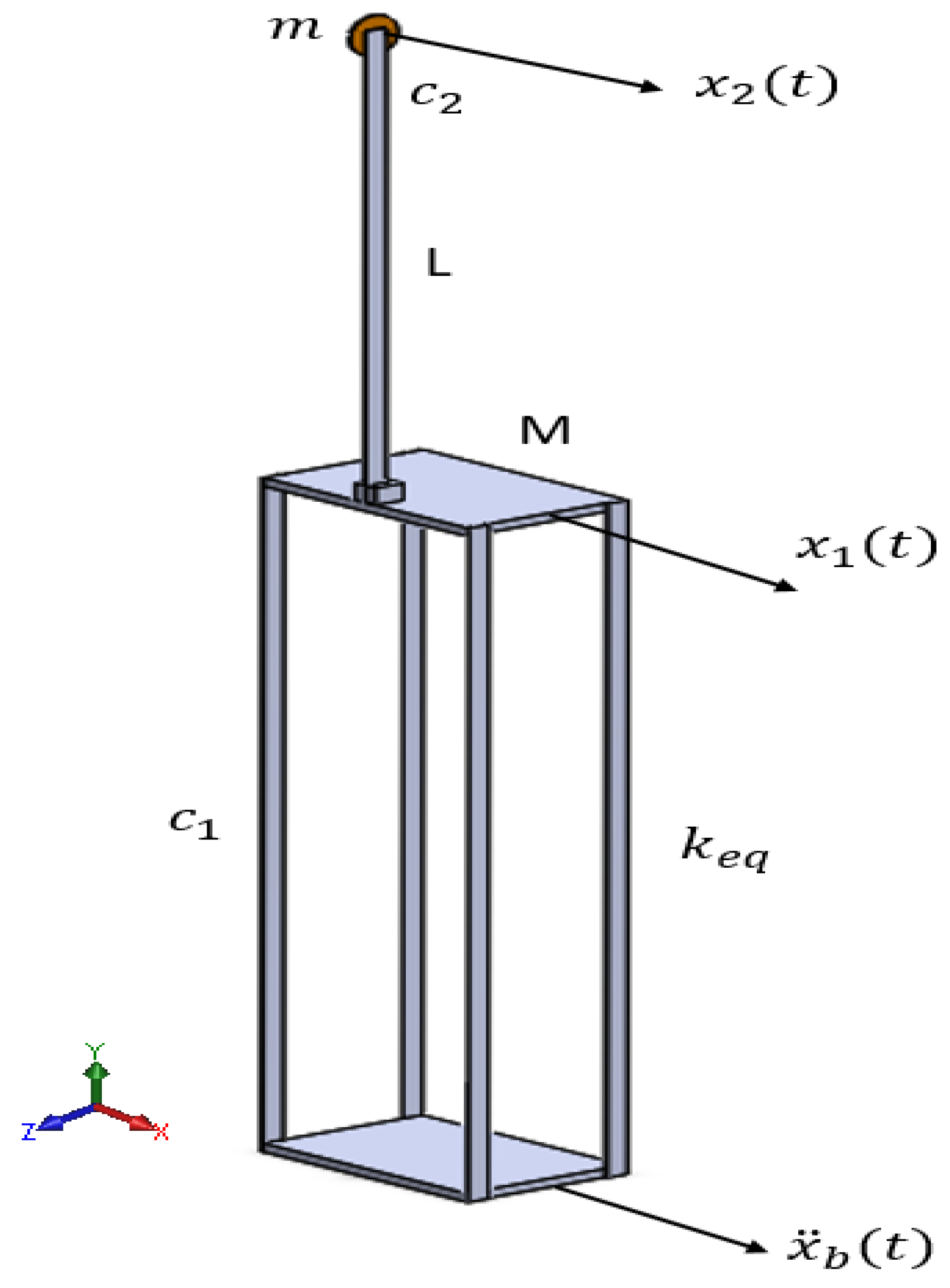
Figure 1 depicts a schematic diagram of the mechanical system. The primary system is represented by a building-like structure (discretized in a single degree of freedom) with mass M. It was assumed to be subjected to horizontal ground motion perturbation . Vertical columns were assumed to be weightless and inextensible in the vertical direction with equivalent stiffness , while the energy-loss mechanism is represented by viscous damping .
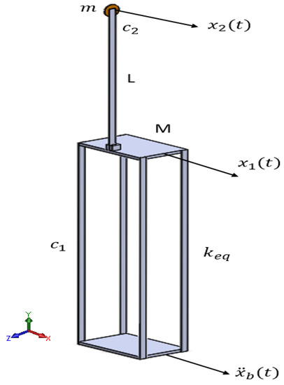
Figure 1.
Schematic representation of building-like structure with flexible vibration absorber.
The flexible absorber is composed of a thin beam attached over the buldinglike structure with equivalent mass m at the end, where its lateral motion is restricted to a vertical plane (i.e., gravity effects are considered). The essential properties of the secondary system (vibration absorber) are flexural stiffness and small viscous damping .
2.1. Equations of Motion
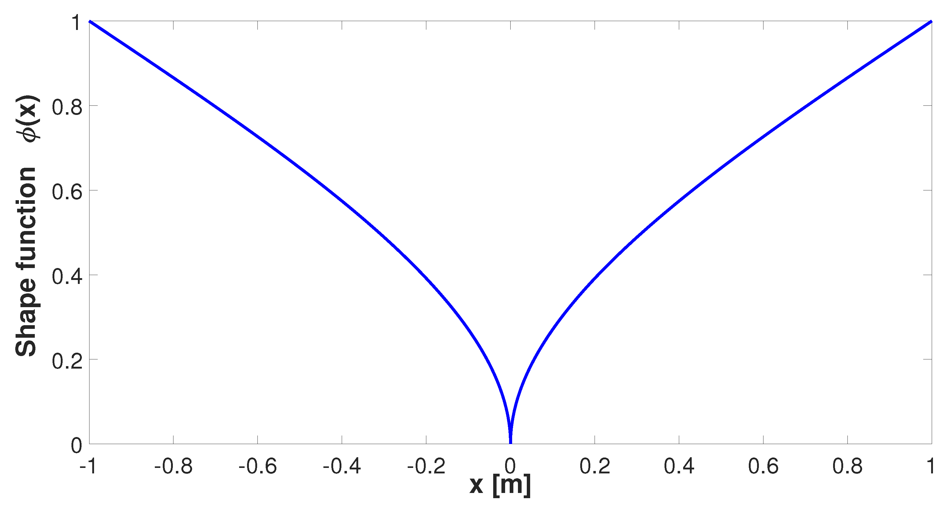
If the secondary system could deform in flexure, it would have an infinite number of degrees of freedom. However, we were only interested in the fundamental vibration mode of the flexible vibration absorber; therefore, it was possible to consider it as a single-degree-of-freedom system, assuming that only one deflection pattern could be developed (generalized SDOF system) [18,19]. The lateral displacement of flexible absorber can be related to center of mass m by using a relationship based on the first mode of linear shape function [20]; thus,
where is the tip displacement of the secondary system. For this case, is obtained from the deflection curve of a cantilever beam with a concentrated load at the endpoint (see Figure 2) given by
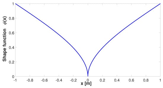
Figure 2.
Deflection pattern considered for the flexible vibration absorber.
The equations of motion for the building-like structure with flexible vibration absorber (two-degree-of-freedom system) were obtained via an energy approach. Kinetic energy and potential energy are given by
where , w, and g denote the longitudinal motion of the primary system, the axial contribution displacement of tip mass m, and gravitational acceleration, respectively. The potential energy consisted of strain energy because of beam bending and the gravitational potential energy of the tip mass.
w can be directly related to lateral displacement by [20,21]:
According to the Euler–Lagrange equations, the dynamics of the complete system is given by
where is the vector of exogenous forces with , where A is the amplitude of the ground motion, and is close to the resonant frequency of the building-like structure. Upon substituting (6) into (7), the dymamics of the system shown in Figure 1 can be described as follows:
If the nonlinear terms are neglected, the system given by (8) and (9) can be rewritten as
where , and M, C, K are given by
By taking the Laplacian transform of both sides of (10), neglecting initial conditions of the linear vibrating system model, we obtain
This leads to transfer function
The substitution of Equation (11) in (13) leads to
from which we obtain the transfer functions of the system:
where corresponds to the transfer function from input to coordinate ; is the transfer function from input to coordinate ; and is a polynomial of 4th order given by
with
By taking the inverse Laplacian transform of Equation (14), it is possible to find the outputs of system (, ) in the time domain for any known input .
2.2. Tuning Condition
The main purpose of the flexible vibration absorber is to attenuate the resonant response of the primary system due to harmonic excitation at its base. In order to determine the length value associated with the secondary system that allows for achieving the aforementioned objective, the following frequency transfer function is obtained from (considering ):
If the numerator of Equation (16) is equal to zero (necessary condition to cancel the dynamic response of the primary system), the following expression is obtained:
Because the building-like structure operates under resonant conditions (), the flexible vibration absorber was designed so that
For simplicity, the length of the flexible vibration absorber was chosen as the tuning parameter; its value is given by the real root of the next polynomial equation:
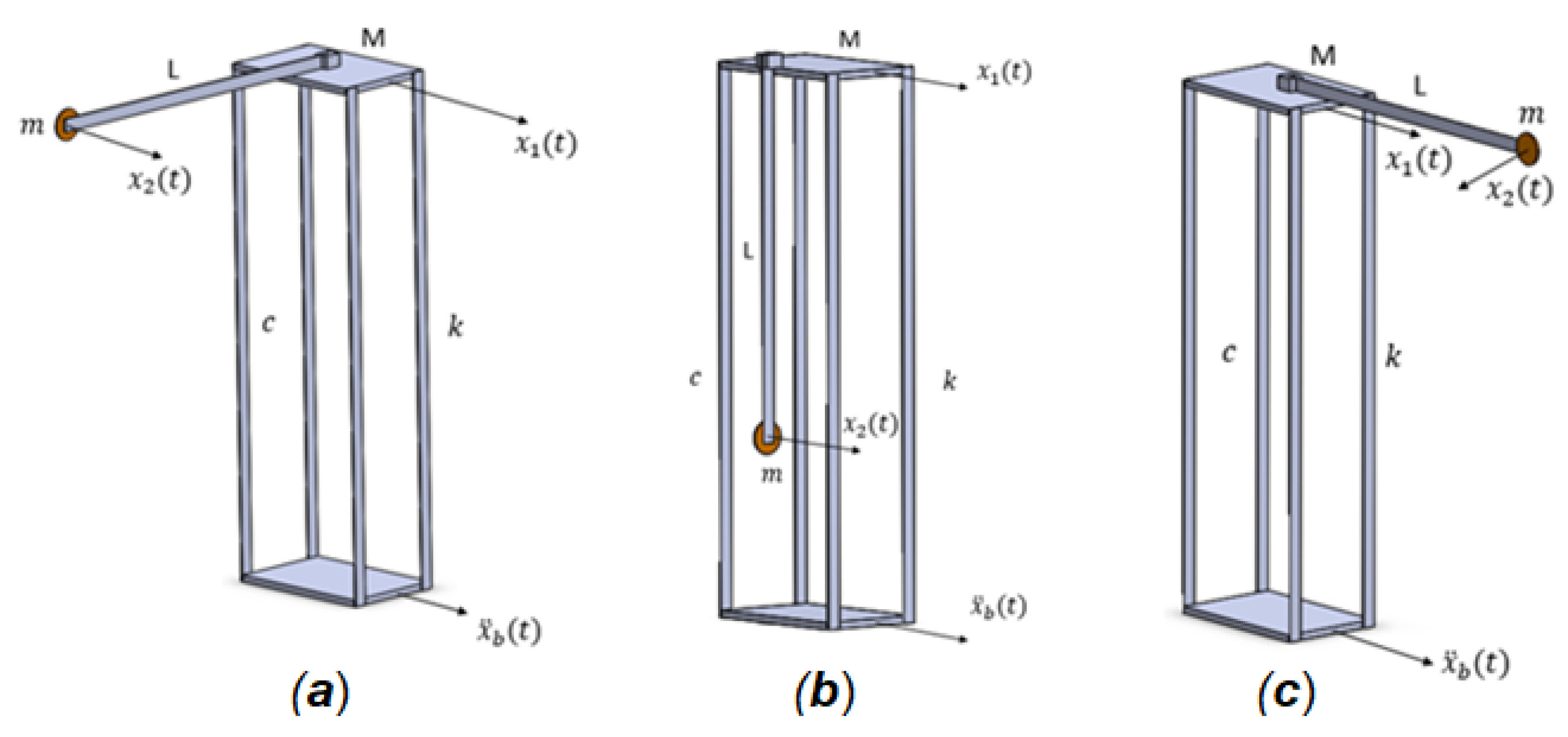
2.3. Other Possible Configurations of Flexible Vibration Absorber
It is possible to implement the proposed flexible vibration absorber in three additional configurations (see Figure 3). In the first, the dynamics of the secondary system occurs in a horizontal plane; therefore, the potential energy associated with mass m is negligible. The second is very similar to the configuration shown in Figure 1; the only difference is that the potential energy associated with the tip mass m is now positive. Lastly, the third configuration has the characteristic that the main axis of the flexible vibration absorber is parallel to the direction of the perturbation signal.
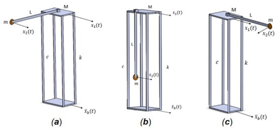
Figure 3.
Different possible configurations of FVA: (a) no potential energy, (b) positive potential energy, (c) autoparametric version.
Considering the change because of the term associated with the potential energy of mass m, it is possible to use the Lagrangian of the system given in (6) to obtain the dynamic model of the first two configurations shown in Figure 3. If the Euler–Lagrange equations are applied (see Equation (7)), the equations of motion are described by
- Configuration
- Configuration
The only difference between linearized models is the value of the last element in the stiffness matrix; therefore, the tuning condition Equation (19) can be used to determine the value of the length of the flexible vibration absorber in any of its configurations, where a linear behavior of the overall system is considered.
On the other hand, configuration corresponds to an autoparametric system, where the dynamic model is represented by a system of nonlinear differential equations that cannot be linearized due to the decoupling between the degree of freedom of the primary system and the dynamics of the absorber to be implemented [22,23]. This kind of configuration is not considered in the present work due to it having been widely studied in the nonlinear-vibrations literature, addressing passive and active control aspects for different hosting structures [24,25,26,27,28,29,30,31,32,33,34,35,36,37].
2.4. Simulation Results
In order to show the performance of the flexible vibration absorber coupled to the building-like structure (configuration depicted in Figure 1), some simulations were performed considering both dynamic models (see Equations (8)–(10)). The considered parameters of the overall system are presented in Table 1.

Table 1.
System parameters.
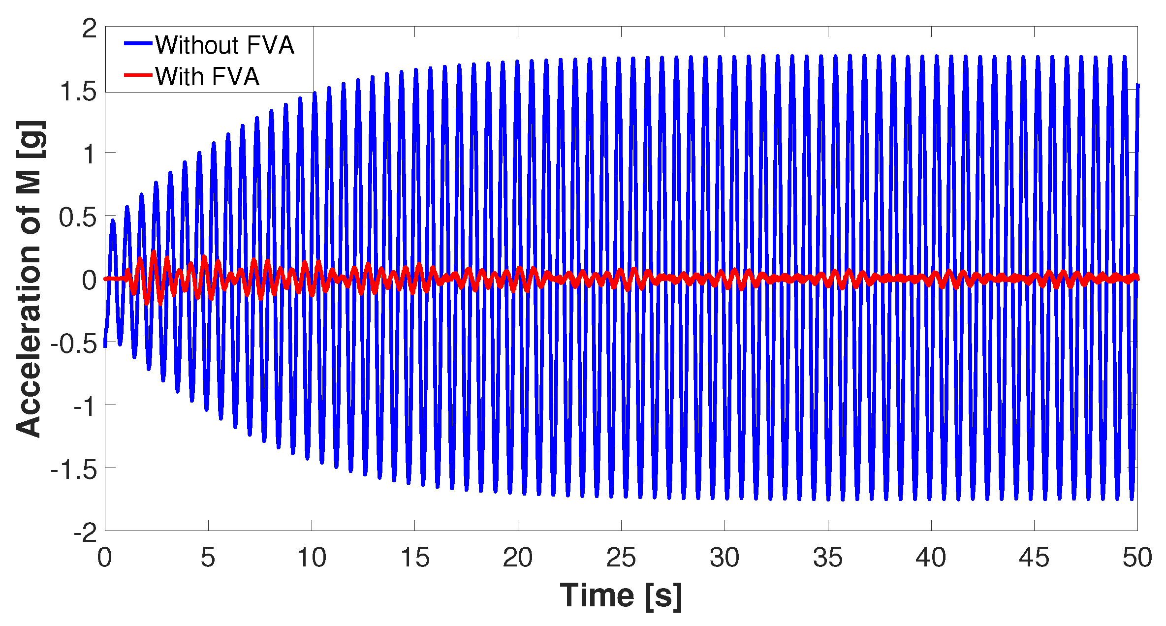
Figure 4 shows a comparison of the dynamic response of the building-like structure without and with flexible vibration absorber when . When the secondary system was tuned, the displacement of the primary system was very similar in both dynamic models, with a vibration absorption percentage higher than .
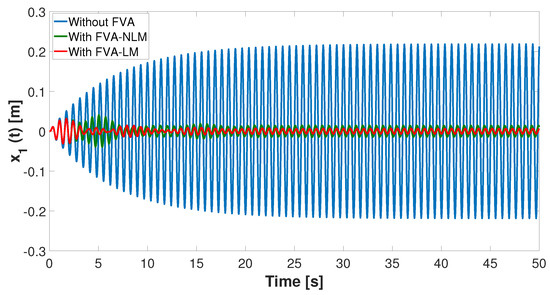
Figure 4.
Dynamic response of primary system with and without FVA.
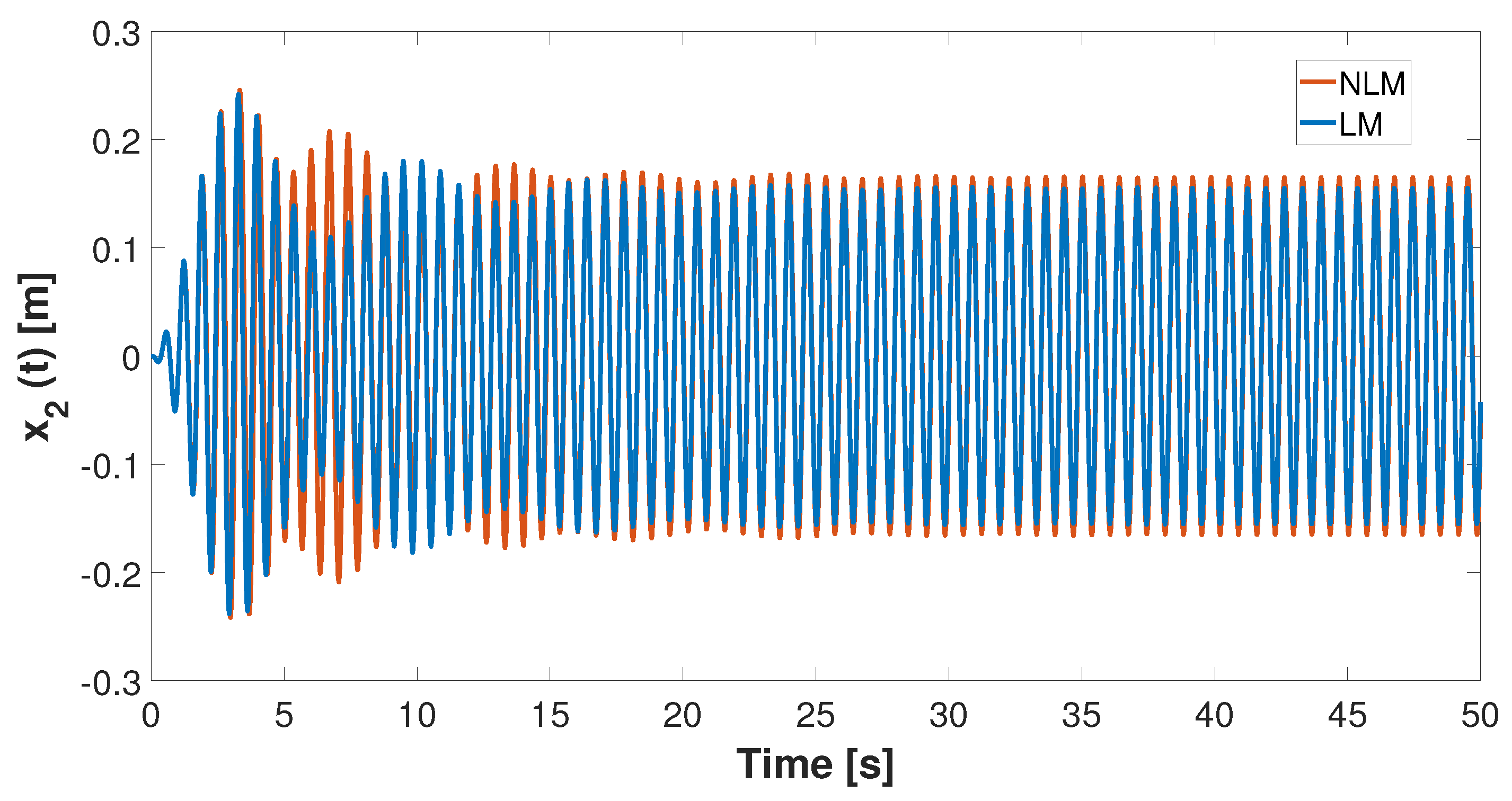
The response of the secondary system when it was tuned to passively attenuate resonant vibrations in the main system is described in Figure 5. The steady-state vibration amplitude was close to 16 cm in both dynamic models.

Figure 5.
Dynamic response of secondary system when .
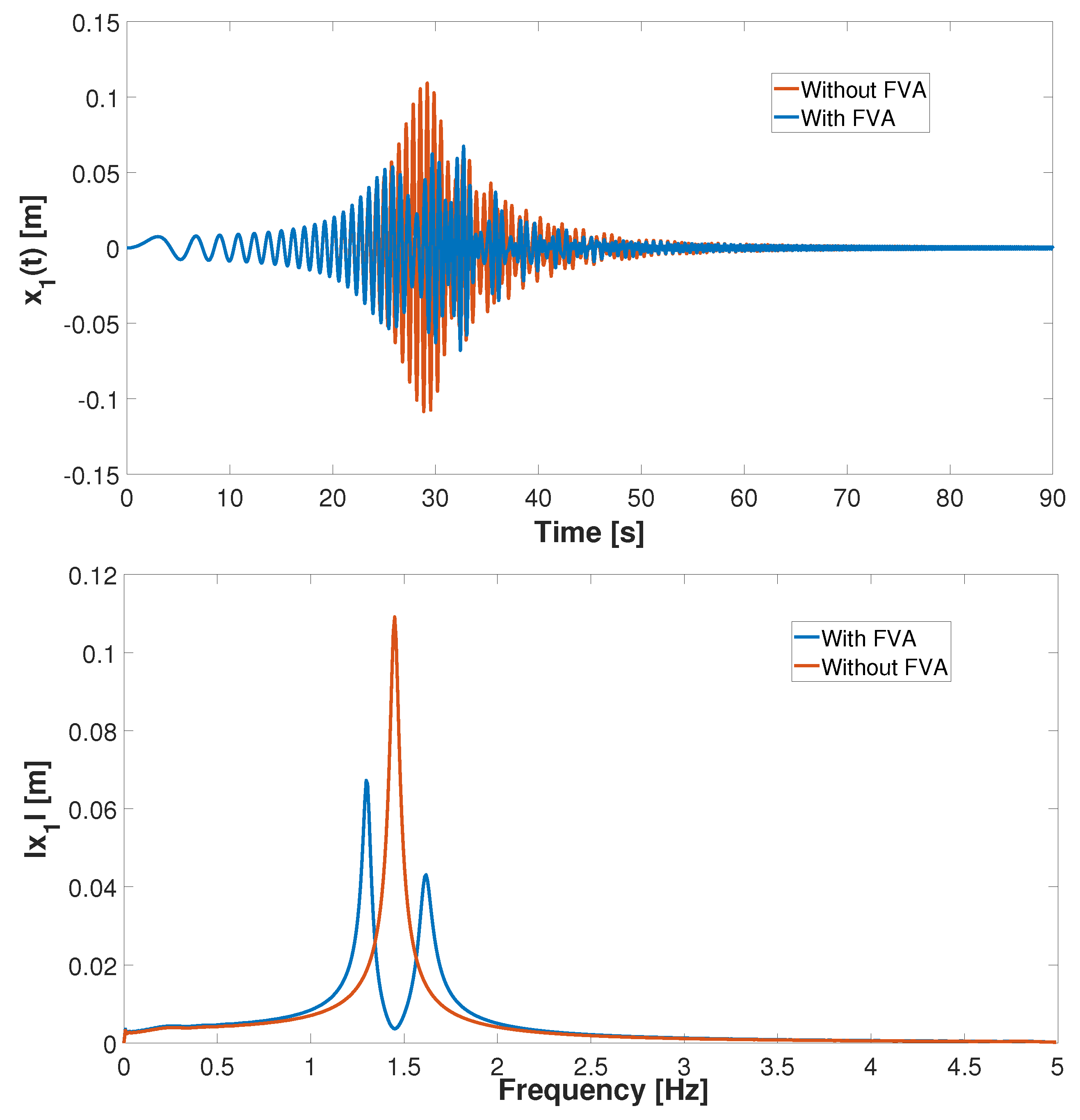
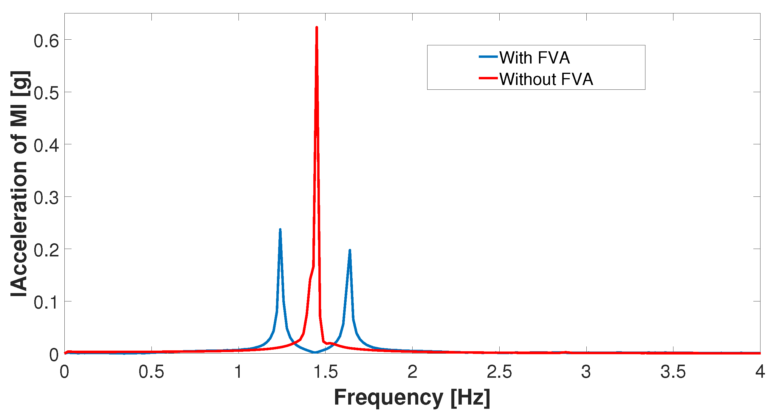
Figure 6 shows the dynamic response of the primary system (with and without flexible vibration absorber) in the time and frequency domains when it was excited on its base with a sine sweep from 0 to 5 Hz during 90 s. There was an antiresonance frequency exactly in the design frequency of the secondary system, while a pair of natural frequencies were generated around this value. This is a well-known dynamic condition in the design and implementation of passive vibration absorbers with inertial or elastic coupling between both subsystems [1].
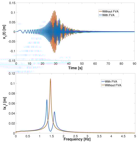
Figure 6.
Dynamic behavior of building-like structure under sine sweep. (top) Time domain; (bottom) frequency domain.
Quantification and Detection of Nonlinear Behavior
The optimal performance of the proposed flexible vibration absorber occurs when the complete system describes dominantly linear behavior around its nominal operating conditions or maximal allowable deflections. This assumption was established in Equation (12), which implies the application of a linear operator; in this specific case, the Laplace transform. Even though the absorber had a nonlinear model, it was considered to behave as a linear system in spite of the nonlinear phenomena as established in Equations (8) and (9). On the other hand, analysis of the Hilbert transformation of the frequency response of a given system is a practical and well-founded nonlinearity analysis technique [38,39,40,41]. In this section, we apply Hilbert transformation operator [38] to the simulated frequency response functions () of two cases: the primary system without any vibration absorber, and the complete system, including the flexible vibration absorber, using nonlinear models (8) and (9) in order to numerically determine the influence of the nonlinear part of the model over the complete dynamic response. As defined in [36,38,39,40,41] and references therein, the Hilbert transformation of a particular is given by
where denotes the Hilbert transformation operator, term is the Cauchy principal value of the integral, and denotes frequency. The Cauchy principal value is necessary due to the presence of the singularity at in the integrand.
The Hilbert transformation applied to frequency response functions of mechanical systems offers a method for detecting and quantifying the presence of nonlinear behavior by using the simplified criterion [41]:
This implies that the of a linear system is not distorted or altered by Hilbert transform operator , whereas Hilbert transform operator applied to the of a nonlinear system produces a distorted version of the original [36,38,39,40,41].
By using the properties of the Hilbert transform exposed before, there exists a set of nonlinearity indicators of indices, explained well and reported in [41], which determine and quantify the distortion on the original FRF under the action of the Hilbert transformation operator. In this work, we use the nonlinearity index reported in [42], which is based on the cross-correlation coefficient defined by
where is the original of the system, H is the Hilbert transformation of , is the bandwidth of interest with , and expression is the cross-correlation coefficient. Therefore, the value of is used as a nonlinearity indicator or index that constitutes a numerical quantifier of the presence of nonlinear behavior in a particular mechanical system, considering its operating conditions and design specifications. Considering that the Hilbert transformation in an experimental context is performed by using numerical methods, we need to specify linearity or nonlinearity criteria. Hence, as reported in [36,39,41,42], it is appropriate to consider a value of for a correct assumption of linear dynamic behavior for the system.
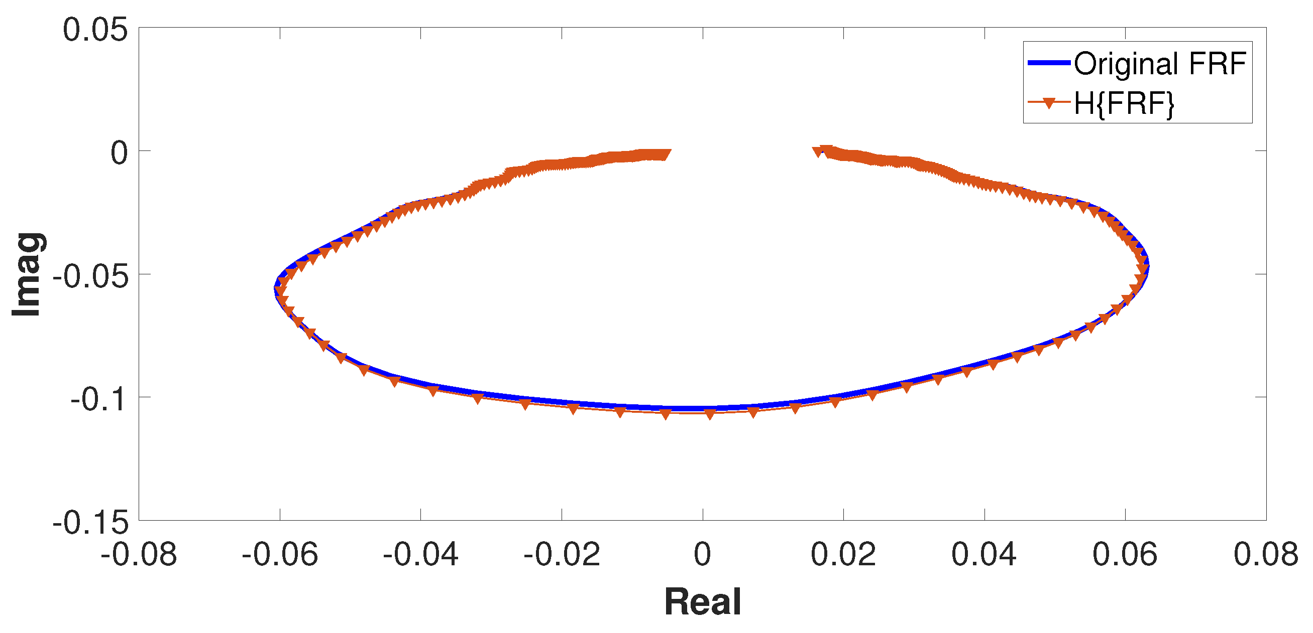
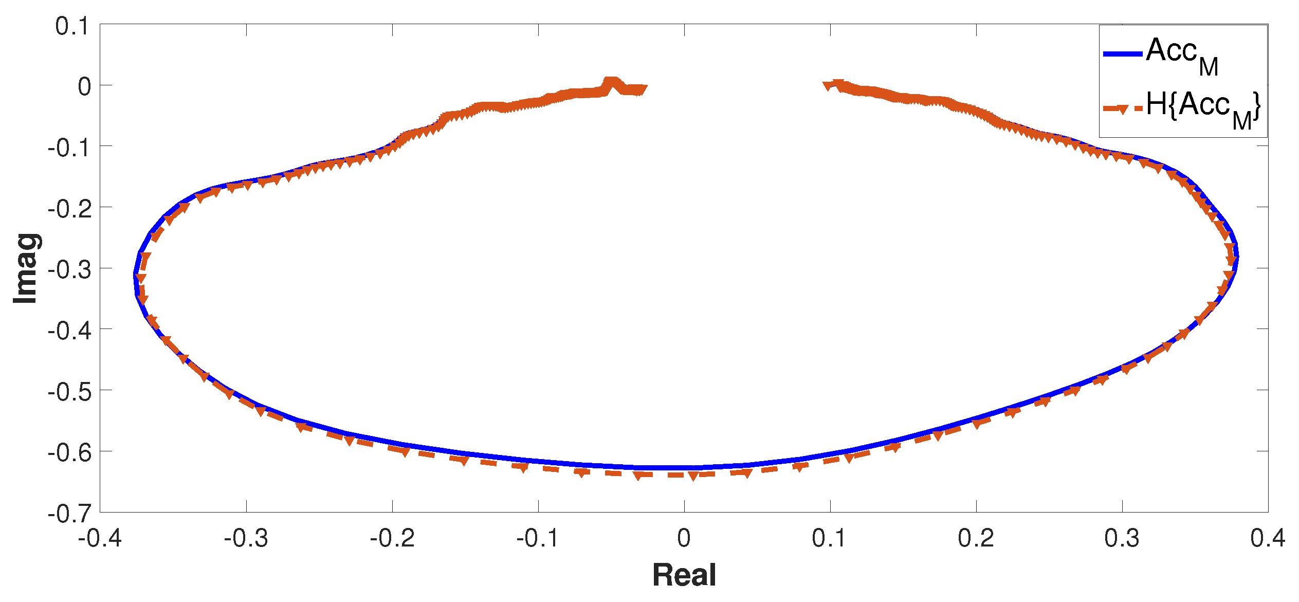
The nonlinearity detection approach proposed here is valid for any obtained by measurements of position , velocity or acceleration , with i as a specific output under analysis. Consider the frequency domain chart shown in Figure 6 where both are depicted: in orange, the of the primary system without any vibration absorber; in blue, the of the system with the vibration absorber attached to it. The Argand diagram of the primary system without any absorber is shown in Figure 7. The graph of the original under Hilbert transformation operator (in orange and dotted line) did not generate a distorted version of the ; then, as expected, the primary system was dominantly linear.
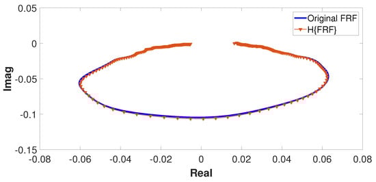
Figure 7.
Original (blue line) and corresponding Hilbert transformation (dotted orange line) of the primary system without any vibration absorber.
The numerical result of the nonlinearity index defined by Equation (28), applied to the of the primary system is
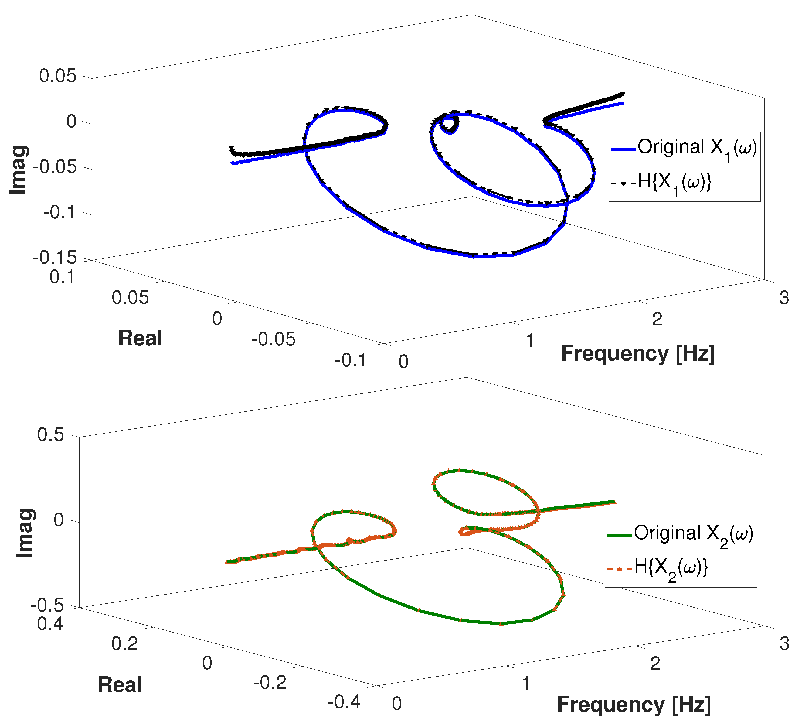
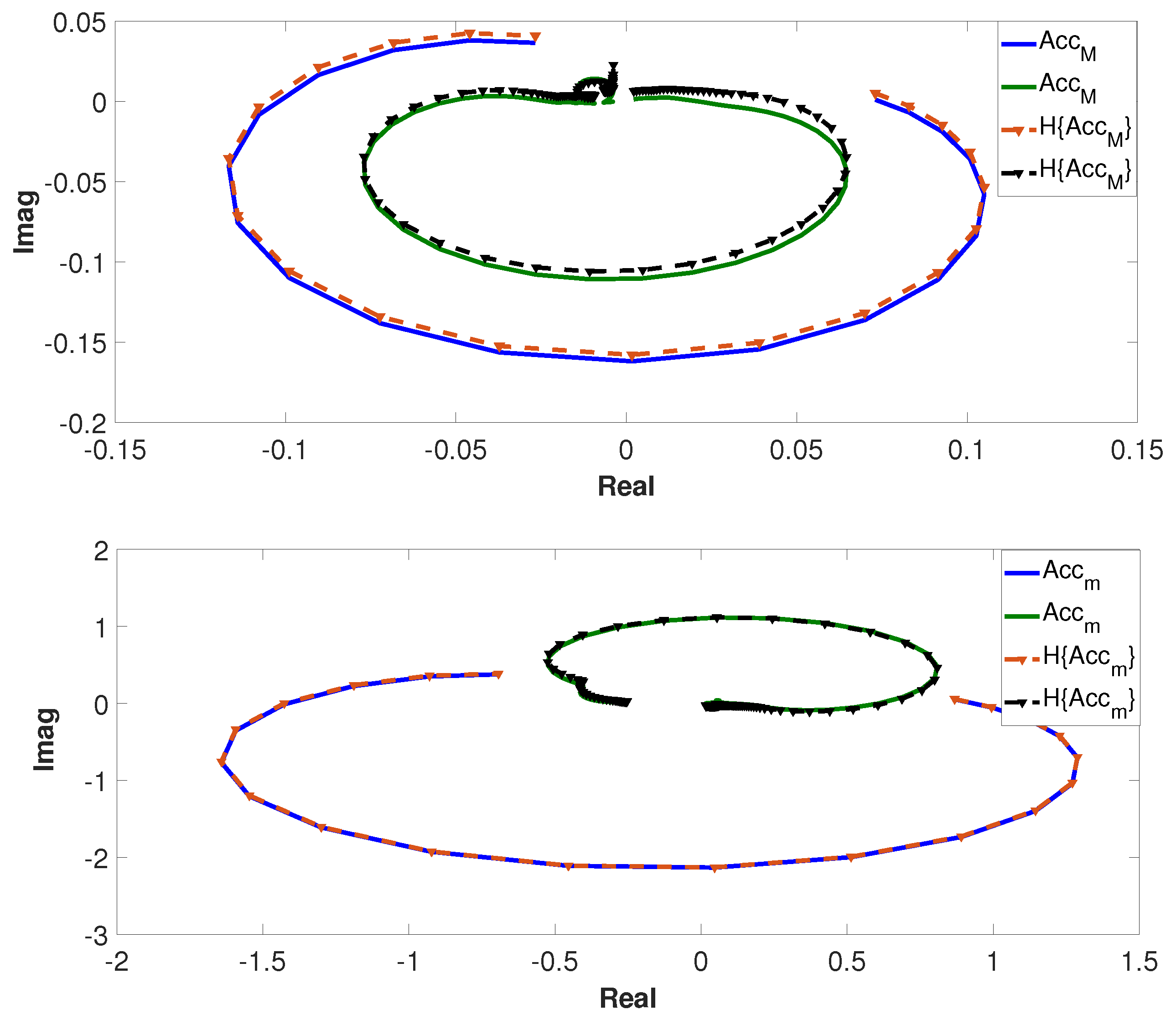
Now, consider the shown in Figure 6 (blue line), which corresponds to the system with the vibration absorber attached to the primary system. The Argand diagram of Figure 8 shows the comparison between the original (blue line) and the result of the application of the Hilbert transform (black dashed line) in a three-dimensional Nyquist diagram; the graphs correspond to analysis based on the Hilbert transform of the two main of the system y , where is the of the primary system, and is the mass of the flexible absorber. The numerical result of the nonlinearity indices calculated with Expression (28) are reported in Table 2.
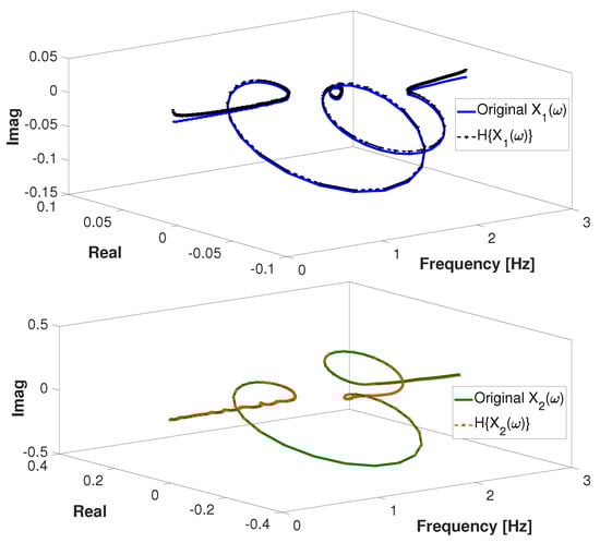
Figure 8.
Hilbert transform analysis. corresponds to the primary system, and to the mass attached to the flexible vibration absorber.
Table 2.
Calculated nonlinearity indices.
The nonlinearity criterion used to consider a system as predominantly linear, as mentioned before, is . Therefore, the considered system was predominantly linear with and without the presence of the flexible vibration absorber in the simulated operating conditions.
In the Argand diagram shown in Figure 8, it is possible to notice the phase change for the movement of the absorber. When the two masses of system M and m are in phase, the imaginary part is negative, and the phase change is noted in the positive value of the imaginary part in the semicircle that is formed in the vicinity of the resonance.
3. Experimental Results
In order to validate the effectiveness of the flexible vibration absorber attached to the building-like structure, some experiments were performed.
3.1. Modal Parameter Identification—Primary System
First, it is necessary to determine the modal parameters corresponding to the primary system to know the value of its natural frequency and damping ratio. The main system was placed on a Stewart platform (Quanser Hexapod), and a free vibration test was conducted (see Figure 9). A small low-power triaxial accelerometer (ADXL335) was used to measure the acceleration of mass M. Sensor reading was conducted by using an Arduino due microcontroller that had been programmed in Python with a sampling rate of 5 kHz.
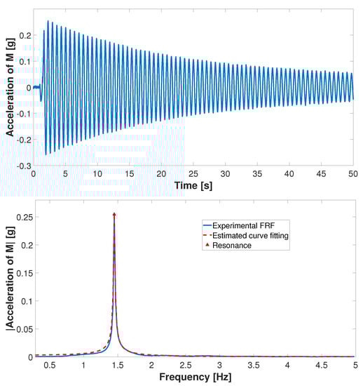
Figure 9.
Dynamic behavior of building-like structure under initial condition of perturbation. (top) Time domain; (bottom) frequency domain.
The modal parameters of the primary system were obtained by using an experimental modal analysis technique [43,44] (peak picking method); their values are given in Table 3.
Table 3.
Modal parameters of building-like structure.
3.2. Primary System with FVA
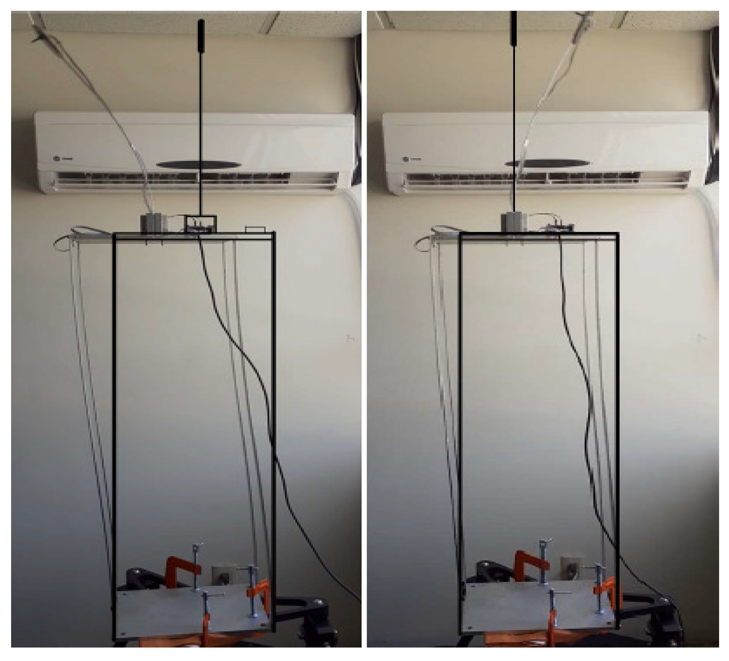
The primary system was a building frame structure with a height of 1 m and a main mass of 2.706 kg, supported by four vertical columns whose bending stiffness in the longitudinal direction was 4.457 Nm2. The secondary system consisted of a cantilever beam with rectangular cross-section () and a tip mass of 0.125 kg. The complete system wa mounted on a Stewart platform to be disturbed under resonant conditions as shown in Figure 10.
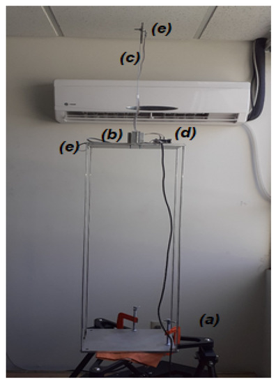
Figure 10.
Experimental setup: (a) Quanser Hexapod; (b) primary system; (c) flexible vibration absorber; (d) microcontroller; (e) accelerometer.
The time history response of the building-like structure with and without FVA when the excitation signal had an amplitude of mm and frequency Hz is described in Figure 11. For this case, the length of the secondary system that allowed for the high percentage of vibration absorption was obtained by solving Equation (19), which resulted in m. Figure 12 describes the experimental response for the secondary system when it was tuned to the building-like structure having a steady-state acceleration amplitude of 1 g.
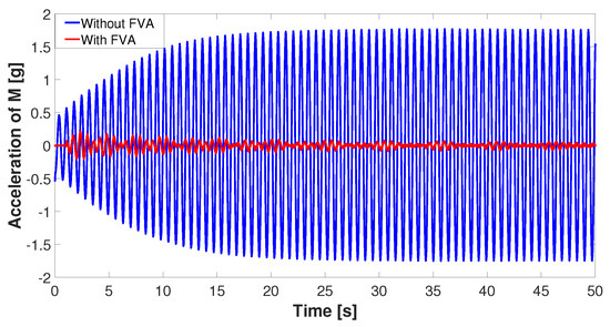
Figure 11.
Acceleration of main system when excitation frequency is .
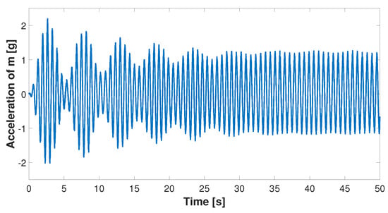
Figure 12.
Acceleration of secondary system when excitation frequency is .
On the other hand, the experimental response of the primary system in the frequency domain with and without FVA is shown in Figure 13. The behavior of the vibration amplitude versus the excitation frequency was very similar to that shown in Figure 6, where a high percentage of vibration absorption was achieved with the disadvantage of generating a pair of resonant frequencies close to the tuning frequency between primary and secondary systems. There was an offset in the frequency response function of the complete system. Therefore, for any possible slight change close to the tuning condition (), the amplitude of motion could present a peak value because of proximity with respect to other resonance frequencies exciting the vibration mode associated with it (see Figure 14).
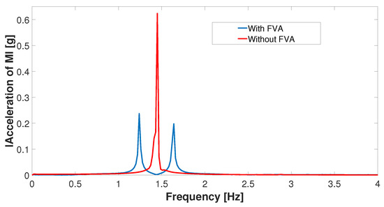
Figure 13.
Experimental frequency response of primary system with and without FVA.
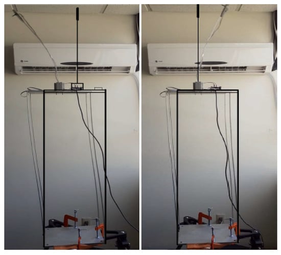
Figure 14.
Vibration modes for overall system. (left side) Mode 1 in phase. (right side) Mode 2 out of phase.
The modal parameters of the system with FVA were obtained by applying the peak picking modal method [43,44] to the experimental shown in Figure 13; their values are given in Table 4.
Table 4.
Modal parameters of structure with FVA.
Even when the inclusion of the FVA had the effect of introducing a new resonance, as shown in Figure 13, the damping ratio was considerably higher for both resonances for the system with the absorber, as reported in Table 4. In the same way, a considerable reduction in the amplitude of the resonant response was seen compared to the system without the absorber, which is also evident in the graph of Figure 13. Comparative analysis to quantify the differences in percentage terms between the modal parameters of the system with and without FVA is shown in Table 5.
Table 5.
Modal parameter comparison.
In addition to the reduction in the modal amplitude of the , the change in the natural frequency of the primary system without any type of absorber generated a change in the dynamic response that enhanced the performance of the system in operational terms.
Quantification and Detection of Nonlinear Behavior
In order to experimentally determine the presence of nonlinearities in the vibrating response of the system, we applied Hilbert transform analysis of the experimental shown in Figure 13, obtained with measurements of acceleration. Regarding the theory and practice of modal analysis, the main premise is decoupling the differential equations typical of mathematical models in vibrating mechanical systems; the inherent use of principal coordinates for such a decoupling is achieved by expressing the dynamic behavior of the systems under analysis in terms of displacement patterns known as modal shapes, damping ratios, and natural frequencies [43,44]. In the context of modal analysis, velocity, acceleration, and position measurements can be used to experimentally determine the main modal parameters of the systems without loss of accuracy. Then, the nonlinearity index defined by (28) is calculated for two cases: the primary system without a vibration absorber, and considering the complete system including the flexible vibration absorber.
The Argand diagram shown in Figure 15 depicts the comparison between the original of the system without a vibration absorber in the solid blue line and the corresponding Hilbert transformation in dotted lines. The numerical value of the calculated nonlinearity index (28) is
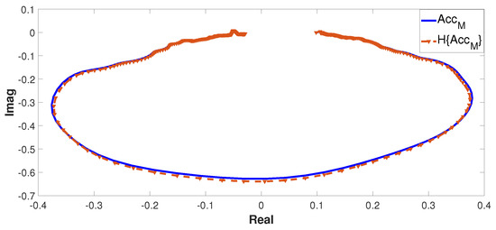
Figure 15.
Experimental Hilbert transformation analysis of primary system without flexible vibration absorber attached to it.
For the second case when the flexible vibration absorber was attached to the primary system, the numerical results of the evaluation of the nonlinearity index (28) are reported in Table 6. The value of the index was very close to 1; therefore, the system was dominantly linear, even in the presence of the flexible vibration absorber at the operating conditions of the test.
Table 6.
Experimental nonlinearity indices.
The Argand diagrams shown in Figure 16 depict the comparison between the original and their corresponding Hilbert transformation versions. The mentioned were obtained with measurements of the acceleration of the primary system and the acceleration of the mass of the flexible vibration absorber; those are denoted as and , respectively. In the same way as in the case of numerical simulation, the phase change in the Argand diagram was visible, as is shown in Figure 16 even when acceleration measurements were used; there existed a clear change in the sign of the imaginary part of the that corresponded to the second degree of freedom or m. The change in the phase in each vibration mode is clearly visible in Figure 14.
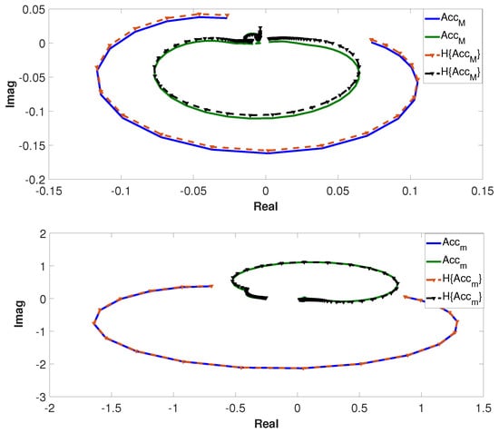
Figure 16.
Experimental Hilbert transformation of system and flexible vibration absorber .
Even though we used displacement measurements in the simulation results presented in Section 2.4, in contrast with the experiments where we used acceleration measurements, Hilbert transform pairs Equations (25) and (26) are still valid, with any dependence on the physical variable used to calculate the nonlinearity index as defined in Equation (28).
4. Conclusions
The passive vibration control of a building-like structure under resonant conditions by using a flexible vibration absorber was presented. Results of the numerical and experimental studies showed that the proposed flexible vibration absorber achieved very good performance in passively attenuating the dynamic response of the primary system in or around its design frequency in any of its possible settings (see Figure 3). From a practical point of view, it is more convenient to implement it in such a way that its dynamics occur in a vertical plane, with its mass above the main mass of the primary system because a shorter design length is required in this configuration. On the other hand, regardless of the type of configuration that is chosen for the flexible vibration absorber, the main disadvantage is the generation of a pair of natural frequencies around the tuning frequency. For this reason, it is not convenient to apply this type of vibration absorption scheme if the excitation source is not constant or has multiple frequency components. This disadvantage coincides with similar reported schemes in the literature on structural dynamics and passive vibration control methods (e.g., mass-spring damper and pendulum-type absorbers), where this occurs due to the type of coupling, either inertial or elastic, between host structure and secondary system. Even when the complete system that included the action of the flexible vibration absorber presented large deformations, there was predominantly linear behavior; due to this, the performance of the vibration absorber was adequate. The nonlinearity index tested in this work, and based on the Hilbert transform and the correlation coefficient constituted a mathematical tool that gives formality to the experimental verification of the hypothesis about the mostly linear behavior of the overall system.
Author Contributions
Conceptualization, N.F.-M. and H.F.A.-F.; methodology, L.G.T.-F. and F.B.-C.; experimental validation, L.G.T.-F., H.F.A.-F. and A.E.D.-L.; writing—original draft, H.F.A.-F. and L.G.T.-F.; writing—review and editing, F.B.-C. and N.F.-M.; visualization, A.E.D.-L. and D.E.R.-A. All authors have read and agreed to the published version of the manuscript.
Funding
This research was partially supported by Consejo Nacional de Ciencia y Tecnología (CONACYT-México) and Tecnológico Nacional de México (TecNM) projects.
Institutional Review Board Statement
Not Applicable.
Informed Consent Statement
Not Applicable.
Data Availability Statement
Not Applicable.
Conflicts of Interest
The authors declare no conflict of interest.
Abbreviations
The following abbreviations are used in this manuscript:
| FVA | Flexible vibration absorber |
| LM | Linear model |
| NLM | Nonlinear model |
References
- Korenev, B.G.; Reznikov, L.M. Dynamic Vibration Absorber: Theory and Technical Applications; Wiley: London, UK, 1993. [Google Scholar]
- Preumont, A.; Seto, K. Active Control of Structures; John Wiley & Sons: Chichester, UK, 2008. [Google Scholar]
- Enríquez-Zárate, J.; Abundis-Fong, H.F.; Velazquez, R.; Gutierrez, S. Passive vibration control in a civil structure: Experimental results. Meas. Control 2019, 52, 938–946. [Google Scholar] [CrossRef]
- Sun, J.Q.; Jolly, M.R.; Norris, M.A. Passive, adaptive and active tuned vibration absorber-a survey. J. Vib. Acoust. 1995, 117, 234–242. [Google Scholar] [CrossRef]
- Frahm, H. A Device for Damping Vibrations of Bodies. U.S. Patent 989,958, 18 April 1911. [Google Scholar]
- Ormondroyd, J.; Den Hartog, J.P. The theory of the dynamic vibration absorber. J. Appl. Mech-T ASME 1928, 50, 9–22. [Google Scholar]
- Den Hartog, J.P. Mechanical Vibrations; McGraw-Hill: New York, NY, USA, 1956. [Google Scholar]
- Brownjohn, J.M.W.; Carden, E.P.; Goddard, C.R.; Oudin, G. Real-time performance monitoring of tuned mass damper system for a 183 m reinforced concrete chimney. J. Wind Eng. Ind. Aerodyn. 2010, 98, 169–179. [Google Scholar] [CrossRef]
- Elias, S.; Matsagar, V.; Datta, T.K. Effectiveness of distributed tuned mass dampers for multi-mode control of chimney under earthquakes. Eng. Struct. 2016, 124, 1–16. [Google Scholar] [CrossRef]
- Belver, A.V.; Magdaleno, Á.; Brownjohn, J.M.W.; Lorenzana, A. Performance of a TMD to Mitigate Wind-Induced Interference Effects between Two Industrial Chimneys. Actuators 2021, 10, 12. [Google Scholar] [CrossRef]
- Elias, S.; Matsagar, V. Research developments in vibration control of structures using passive tuned mass dampers. Annu. Rev. Control 2017, 44, 129–156. [Google Scholar] [CrossRef]
- Yang, F.; Sedaghati, R.; Esmailzadeh, E. Vibration suppression of structures using tuned mass damper technology: A state-of-the-art review. Int. J. Dyn. Control 2021, 4, 1077546320984305. [Google Scholar] [CrossRef]
- Kavyashree, B.; Patil, S.; Rao, V.S. Review on vibration control in tall buildings: From the perspective of devices and applications. Int. J. Dyn. Control 2021, 9, 1316–1331. [Google Scholar] [CrossRef]
- Wang, W.; Yang, Z.; Hua, X.; Chen, Z.; Wang, X.; Song, G. Evaluation of a pendulum pounding tuned mass damper for seismic control of structures. Eng. Struct. 2021, 228, 111554. [Google Scholar] [CrossRef]
- Pozos-Estrada, A.; Hong, H.P. Sensitivity analysis of the effectiveness of tuned mass dampers to reduce the wind-induced torsional responses. Lat. Am. J. Solids Struct. 2015, 12, 2520–2538. [Google Scholar] [CrossRef] [Green Version]
- Jin, C.; Chung, W.C.; Kwon, D.S.; Kim, M. Optimization of tuned mass damper for seismic control of submerged flotating tunnel. Eng. Struct. 2021, 241, 112460. [Google Scholar] [CrossRef]
- Wielgos, P.; Gerylo, R. Optimization of Multiple Tuned Mass Damper (MTMD) Parameters for a Primary System Reduced to a Single Degree of Freedom (SDOF) through the Modal Approach. Appl. Sci. 2021, 11, 1389. [Google Scholar] [CrossRef]
- Clough, R.W.; Penzien, J. Dynamics of Structures, 2nd ed.; McGraw-Hill: New York, NY, USA, 1993. [Google Scholar]
- Chopra, A.K. Dynamics of Structures; Prentice-Hall: Englewood Cliffs, NJ, USA, 2001. [Google Scholar]
- Esmailzadeh, E.; Nakhaie-Jazar, G. Periodic behavior of a cantilever beam with end mass subjected to harmonic base excitation. Non-Linear Mech. 1998, 33, 567–577. [Google Scholar] [CrossRef]
- Meirovitch, L. Analytical Methods in Vibrations; Macmillan: New York, NY, USA, 1967. [Google Scholar]
- Cartmell, M.O. Introduction to Linear, Parametric and Nonlinear Vibrations; Chapman and Hall: London, UK, 1990. [Google Scholar]
- Tondl, A.; Ruijgrok, T.; Verhulst, F.; Nabergoj, R. Autoparametric Resonance in Mechanical Systems; Cambridge University Press: Cambridge, MA, USA, 2000. [Google Scholar]
- Haxton, R.S.; Barr, A.D.S. The Autoparametric Vibration Absorber. ASME J. Eng. Ind. 1972, 94, 119–124. [Google Scholar] [CrossRef]
- Ibrahim, R.A.; Barr, A.D.S. Autoparametric resonance in a structure containing liquid, Part 1: Two mode interaction. J. Sound Vib. 1975, 42, 159–179. [Google Scholar] [CrossRef]
- Ibrahim, R.A.; Li, W. Structural modal interaction with combination internal resonance under wide-band random excitation. J. Sound Vib. 1988, 123, 473–495. [Google Scholar] [CrossRef]
- Zhimiao, Y.; Haithem, E.T.; Ting, T. Nonlinear characteristics of an autoparametric vibration system. J. Sound Vib. 2017, 390, 1–22. [Google Scholar]
- Mahmoudkhani, S. Improving the performance of auto-parametric pendulum absorbers by means of a flexural beam. J. Sound Vib. 2008, 425, 102–123. [Google Scholar] [CrossRef]
- Silva-Navarro, G.; Abundis-Fong, H.F. Passive/active autoparametric cantilever beam absorber with piezoelectric actuator for a two-story building-like structure. J. Vib. Acoust. 2015, 2015, 011012. [Google Scholar] [CrossRef]
- Abundis-Fong, H.F.; Enríquez-Zárate, J.; Cabrera-Amado, A.; Silva-Navarro, G. Optimum Design of a Nonlinear Vibration Absorber Coupled to a Resonant Oscillator: A Case Study. Shock Vib. 2018, 137, 1–11. [Google Scholar] [CrossRef] [Green Version]
- Ibrahim, R.A.; Yoon, Y.J.; Evans, M.G. Random excitation of nonlinear coupled oscillation. Nonlinear Dyn. 1990, 1, 91–116. [Google Scholar] [CrossRef]
- Enriquez-Zarate, J.; Abundis-Fong, H.F.; Silva-Navarro, G. Passive vibration control in a building-like structure using a tuned-mass-damper and an autoparametric cantilever beam absorber. In Active and Passive Smart Structures and Integrated Systems 2015; International Society for Optics and Photonics: Washington, DC, USA, 2015; Volume 9431. [Google Scholar]
- Silva-Navarro, G.; Abundis-Fong, H.F. Evaluation of Autoparametric Vibration Absorbers on N-Story Building-Like Structures. In Nonlinear Dynamics, Volume 1; Conference Proceedings of the Society for Experimental Mechanics Series; Kerschen, G., Ed.; Springer: Cham, Switzerland, 2017; pp. 177–184. [Google Scholar]
- Flores-Sanchez, D.A.; Flores-Morita, N.; Campa-Cocom, R.E.; Trujillo-Franco, L.G.; Abundis-Fong, H.F. Attenuation of Vibrations in a Mechanical Oscillator by Implementing Two Types of Vibration Absorbers: Experimental Results. In Proceedings of the International Conference on Mechatronics, Electronics and Automotive Engineering (ICMEAE), Cuernavaca, Mexico, 16–21 November 2020; pp. 104–109. [Google Scholar]
- Zhang, A.; Sorokin, V.; Li, H. Dynamic analysis of a new autoparametric pendulum absorber under the effects of magnetic forces. J. Sound Vib. 2020, 485, 115549. [Google Scholar] [CrossRef]
- Trujillo-Franco, L.G.; Silva-Navarro, G.; Beltran-Carbajal, F.; Campos-Mercado, E.; Abundis-Fong, H.F. On-Line Modal Parameter Identification Applied to Linear and Nonlinear Vibration Absorbers. Actuators 2020, 9, 119. [Google Scholar] [CrossRef]
- Zhang, A.; Sorokin, V.; Li, H. Energy harvesting using a novel autoparametric pendulum absorber-harvester. J. Sound Vib. 2021, 499, 116014. [Google Scholar] [CrossRef]
- Feldman, M. Hilbert Transform Applications in Mechanical Vibration; John Wiley and Sons, Ltd.: Chichester, UK, 2011. [Google Scholar]
- Tomlinson, G.R. Developments in the use of the Hilbert transform for detecting and quantifying non-linearity associated with frequency response functions. Mech. Syst. Signal Process. 1987, 1, 151–171. [Google Scholar] [CrossRef]
- Worden, K.; Tomlinson, G.R. Nonlinearity in Structural Dynamics: Detection, Identification and Modelling; Institute of Physics Publishing: Bristol, UK; Philadelphia, PA, USA, 2001. [Google Scholar]
- Ondra, V.; Sever, I.A.; Schwingshackl, C.W. A method for detection and characterisation of structural non-linearities using the Hilbert transform and neural networks. Mech. Syst. Signal Process. 2017, 83, 210–227. [Google Scholar] [CrossRef]
- Kragh, K.A.; Thomsen, J.J.; Tcherniak, D. Experimental detection and quantification of structural nonlinearity using homogeneity and Hilbert transform methods. In Proceedings of the International Conference on Noise and Vibration Engineering, Leuven, Belgium, 20–22 September 2010; pp. 3173–3188. [Google Scholar]
- Heylen, W.; Sas, P. Modal Analysis Theory and Testing; Departement Werktuigkunde, Katholieke Universteit Leuven: Leuven, The Netherlands, 2006. [Google Scholar]
- He, J.; Fu, Z.F. Modal Analysis; Butterworth-Heinemann: Oxford, UK, 2001. [Google Scholar]


Publisher’s Note: MDPI stays neutral with regard to jurisdictional claims in published maps and institutional affiliations. |
© 2022 by the authors. Licensee MDPI, Basel, Switzerland. This article is an open access article distributed under the terms and conditions of the Creative Commons Attribution (CC BY) license (https://creativecommons.org/licenses/by/4.0/).