Abstract
The applications of the Eikonal and stationary heat transfer equations in broad fields of science and engineering are the motivation to present an implementation, not only valid for structured domains but also for completely irregular domains, of the meshless Generalized Finite Difference Method (GFDM). In this paper, the fully non-linear Eikonal equation and the stationary heat transfer equation with variable thermal conductivity and source term are solved in 2D. The explicit formulae for derivatives are developed and applied to the equations in order to obtain the numerical schemes to be used. Moreover, the numerical values that approximate the functions for the considered domain are obtained. Numerous examples for both equations on irregular 2D domains are exposed to underline the effectiveness and practicality of the method.
1. Introduction
It is well known that many problems given by non-linear PDEs appear in many fields of science [1,2]. In this paper, due to their importance, the numerical resolution of two of them is proposed: the Eikonal and stationary heat transfer equations. The increasing difficulty to solve these equations, due to the non-linearity of them, makes not only the application of existing numerical methods necessary but also makes the importance of carrying out new numerical methods more suitable for certain equations or domains.
The Eikonal equation is used to describe the behavior of different systems related to control, propagation of waves or environmental phenomena. The Eikonal equation takes the following form
for some function f. H. Zhao proposed a fast sweeping method for computing the numerical solution of the Eikonal equations on a rectangular grid [3], in [4], the authors used a boundary-only meshless method, and in [5], a differential quadrature method was employed. Moreover, a fast marching method is proposed in [6] and a fast semi-Lagrangian method in [7].
The stationary heat transfer equation with thermal conductivity coefficient depending on the coordinates of the domain points and source or sink term describes heat transfer processes when the thermal conductivity is not uniform in the medium and, in addition, there is a heat source. We consider the stationary non-linear heat transfer equation
In (1) and (2), is an open bounded domain in , for . In [8,9,10,11], the authors show several methods for the numerical evaluation of the solutions of the heat transfer equation. Furthermore, in [12], a localized boundary-domain integro-differential equation approach is followed, and a wide summary of numerical methods for solving the stationary heat transfer equation is given in [13].
To the best of our knowledge, a more detailed review of several meshless methods are given in [14]. As an example, in [15], the authors proposed the meshless singular boundary method for anomalous diffusions equations (of particular interest are Remarks 3.2 and 3.3).
The GFDM is a meshless method, as it solves the PDE at each of the points (nodes) where the domain is discretized. Since it does not need integration, it does not need meshing either. Moreover, the addition of nodes for a better approximation of the solution is easy. In irregular domains, it has a great advantage to be able to add nodes in the subdomains where they are most needed. Obtaining the explicit expressions of the different partial derivatives (explicit formulas) at each node is simple and automatic. Meshless methods have great advantages and, undoubtedly, also disadvantages. Their development and applications have been very important recently. In this paper, we make use of the meshless finite difference approach called Generalized Finite Difference Method (GFDM), which is spreading and is being applied to different fields due to the difficulty of directly solving the partial derivative and time derivative terms on irregular domains. The method was proposed by Lizska and Orkisz [16] and has received great attraction since the paper by Benito et al. [17]. The discretization of the spatial partial derivatives uses a very simple expression (depending only on the distribution of a few nodes, as we explain in the next section), so the treatment of non-linearities is straightforward. For these reasons. a wide range of applications have been recently found [18,19,20]
The paper is organized in the following way. We present some key aspects of the GFDM in Section 2, as well as the application of the Newton–Raphson method. Several computational examples are drawn, and the order of the convergence of the proposed discretization is found. Moreover, the effectiveness of the method is exhibited. Finally, some conclusions are extracted.
2. GFDM and Newton–Raphson Method
2.1. Explicit Finite Difference Formulae
To obtain the explicit formulae of the GFDM, let be a domain in and a discretization of such domain. For the ease of notation and, without loss of generality, let us consider a set of s different points of M, say for a generic interior point of as . Here, with the previous notation, and , define . Different methods, such as distance, quadrant or octant criteria, are usually used to form the stars, see, for instance [17]. By minimizing the residual error of the second-order Taylor series with respect to the spatial partial derivatives at each point of , the explicit difference formulae [17,21] are found, for any regular enough function :
2.2. Newton–Raphson Method (N–R)
We use the Newton–Raphson method for solving system (4).
Let us consider the Jacobian matrix
The N–R method is based on the convergence of the following
where stands for the series of solutionsin the iteration. To define the end of the iterations we consider two different criteria:
- When a given tolerance is reached, in this paper : .
- When 15 iterations are attained.
The initial data is interpolated in the inside of the domain from the Dirichlet condition.
3. Numerical Examples for Eikonal Equation
In order to study the PDE
we use as boundary condition the value of the known solution at those nodes, and we compute the numerical errors with the following
where is the GFD solution and is the exact solution at node i.
3.1. Numerical Test 1
Consider the following PDE
with the exact solution
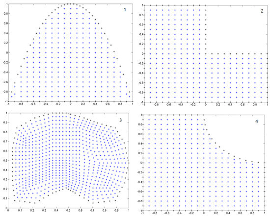
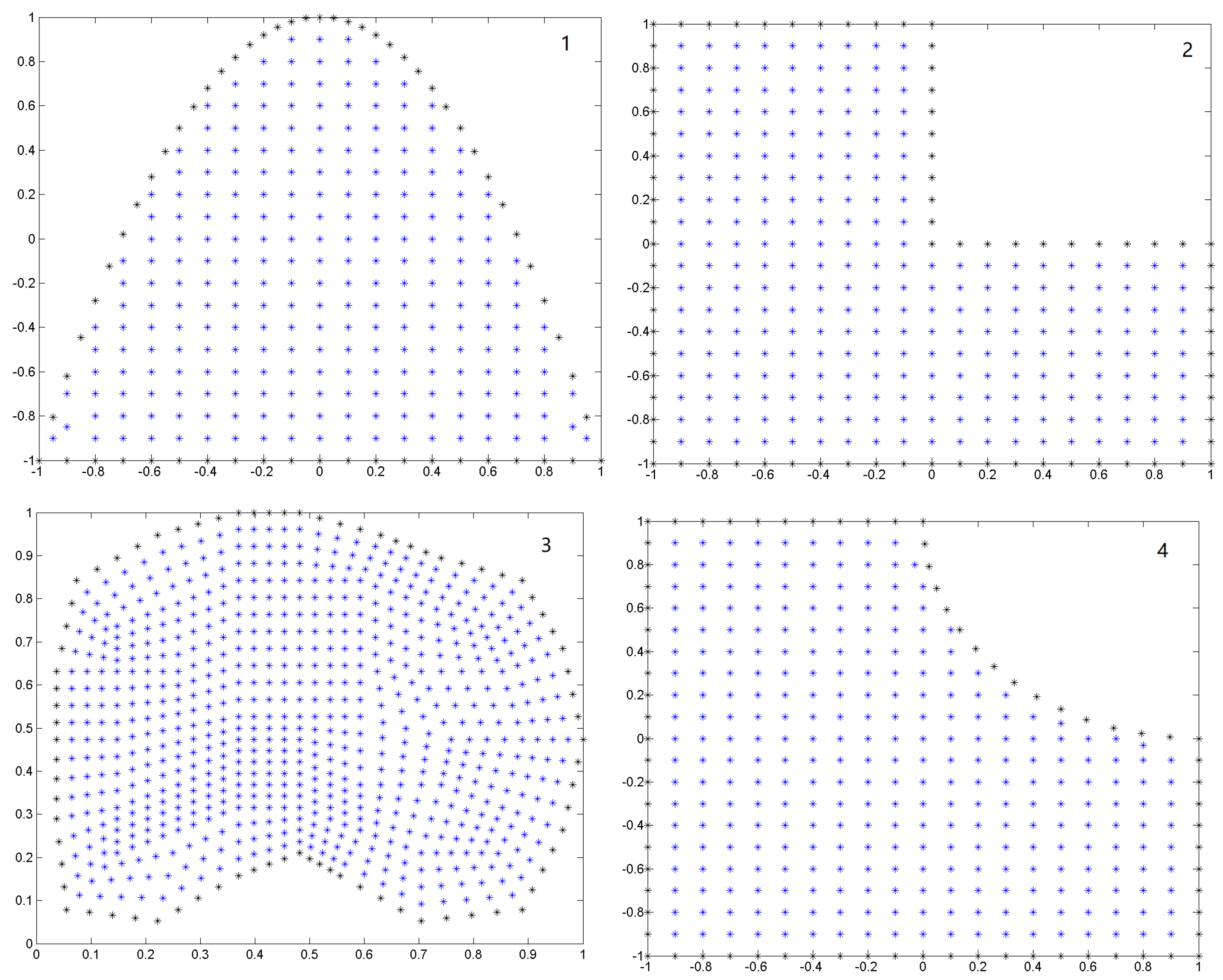
Figure 1.
Irregular clouds for the Examples (1–4).

Table 1.
Error norms for Example 1.
3.2. Numerical Test 2
We solve the PDE
The exact solution is given by the explicit expression
The error norms are illustrated in Table 2.
Table 2.
Error norms for Example 2.
4. Numerical Examples for Stationary Non-Linear Heat Transfer Equation
In this section, we present several numerical results obtained by solving the stationary non-linear heat transfer equation with a source term, where the conductivity is a function of the spatial coordinates, in 2D, with Dirichlet boundary conditions. In particular, we solve the PDE
where is the thermal conductivity and is the source term.
4.1. Numerical Test 3
We consider the stationary non-linear heat transfer equation in the following form
The analytical solution is
In Table 3, the error norms are plotted.
Table 3.
Error norms for Example 3.
4.2. Numerical Test 4
We consider the stationary non-linear heat transfer equation in the following form:
which has the exact solution
Problem (16) is solved on the irregular clouds of Figure 1. In Table 4 the error norms are illustrated.
Table 4.
Error norms for Example 4.
4.3. Convergence Test
In this subsection we provide computational examples showing the numerical order of convergence. We solve the equation
with exact solution
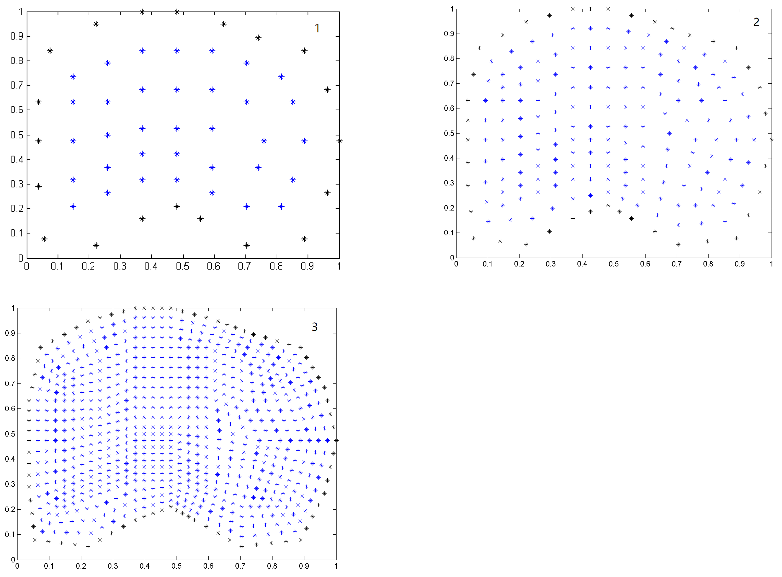
For our purposes, we generate two irregular clouds of points from the third cloud of Figure 1. In Table 5, we show the number of nodes, N, and norms for the three clouds of points in Figure 2, to which we have performed the refinement.
Table 5.
Error norms and for convergence test.
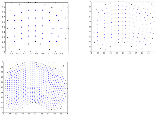
Figure 2.
Refinements 1, 2 and 3.
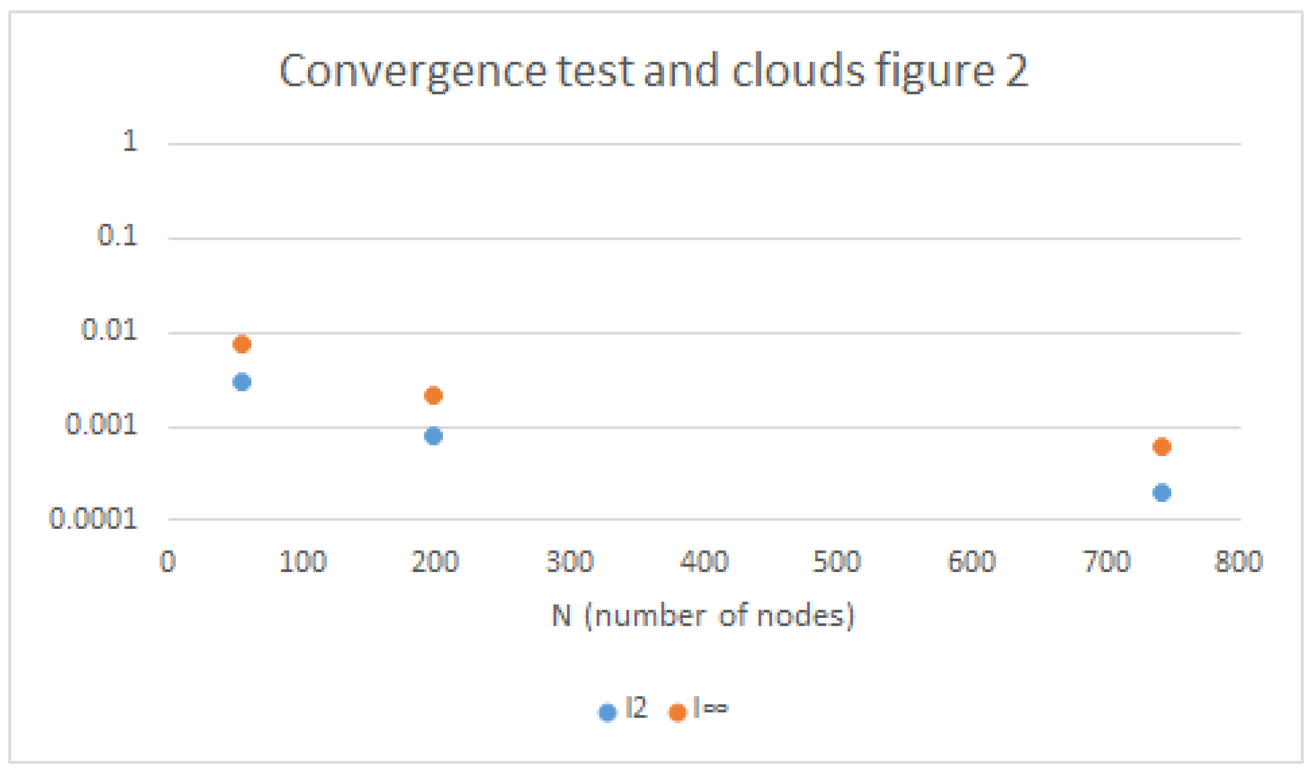
In Figure 3, we display the and norms as functions of the number of nodes N for the three clouds of nodes. The vertical axis of the figures has been plotted on a logarithmic scale.
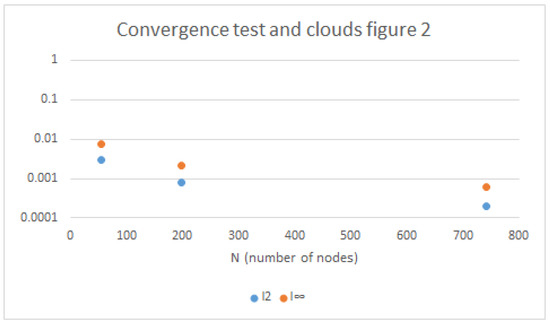
Figure 3.
Refinements vs. error.
5. Example 5: Physical Example
Finally, we proposed a physical example showing the applicability of the above method. To this end, consider the following stationary heat equation
where is the temperature in the square . The boundary conditions are
The solution of the physical example is plotted in Figure 4.
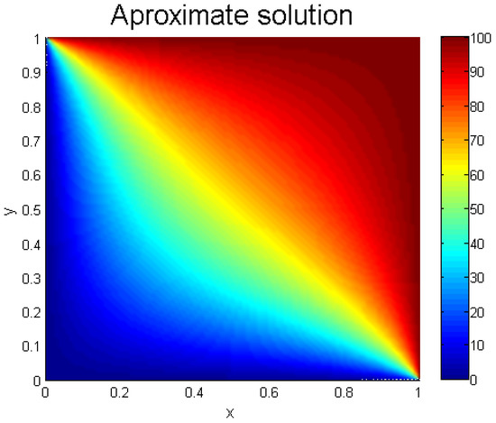
Figure 4.
Solution of Example 5.
6. Conclusions
In order to solve the fully non-linear Eikonal and stationary heat transfer equations, the explicit formulas of the GFDM (Generalized Finite Difference Method) are applied using different irregular clouds of points.
The convenience of using the GFDM meshless method to solve the Eikonal and stationary heat transfer equations are shown by the efficiency and accuracy of the results provided by the application of the method. In fact, the accuracy in the results has been validated in different examples (different domains and solutions).
Apart from applying the method to different domains with irregular clouds, an additional example using the same domain but three different clouds of points (with different point density or refinement) has been studied in order to analyze the convergence of the proposed methodology.
Author Contributions
Conceptualization, M.N. and A.M.V.; methodology, F.U.; software, E.S.; validation, F.U. and A.M.V.; formal analysis, F.U.; investigation, M.N.; resources, Á.G.; data curation, M.N.; writing—original draft preparation, J.F.; writing—review and editing, M.N.; visualization, Á.G.; supervision, F.U.; funding acquisition, F.U. and M.N. All authors have read and agreed to the published version of the manuscript.
Funding
The authors acknowledge the support of the Escuela Técnica Superior de Ingenieros Industriales (UNED) of Spain, project 2021-IFC02. This work is also partially support by the Project MTM2017-83391-P DGICT, Spain.
Institutional Review Board Statement
Not applicable.
Informed Consent Statement
Not applicable.
Data Availability Statement
Not applicable.
Conflicts of Interest
The authors declare no conflict of interest.
References
- Courant, R.; Friedrichs, K.; Lewy, H. On the partial differential eqautions or mathematical physic. Math. Ann. 1928, 100, 32–74. [Google Scholar] [CrossRef]
- Tadmor, A. A review of numerical methods for non-linear partial differential eqautions. Bull. Am. Mthematical Soc. 2012, 42, 507–554. [Google Scholar] [CrossRef] [Green Version]
- Zhao, H. A Fast sweeping Method for Eikonal Equation. Math. Comput. 2004, 74, 603–627. [Google Scholar] [CrossRef] [Green Version]
- Dehghan, M.; Salehi, R. A boundary-only meshless method for numerical solution of the Eikonal equation. Comput. Mech. 2011, 47, 283–294. [Google Scholar] [CrossRef]
- Mehr, M.; Rostamy, D. Computational solutions for Eikonal equation by differential quadrature method. Alex. Eng. J. 2021, 61, 4445–4455. [Google Scholar] [CrossRef]
- Ahmed, S.; Bak, S.; McLaughlin, J.R.; Renzi, D. A Third Order Accurate Fast Marching Method for the Eikonal Equation in Two Dimensions. SIAM J. Sci. Comput. 2011, 33, 2402–2420. [Google Scholar] [CrossRef] [Green Version]
- Cristiani, E.; Falcone, M. Fast Semi-Lagrangian Schemes for the Eikonal Equation and Applications. SIAM J. Numer. Anal. 2007, 45, 1979–2011. [Google Scholar] [CrossRef]
- Crank, J.; Nicolson, E. A practical method for numerical evaluation of solutions of partial differential equations of the heat-conduction type. Adv. Comput. Math. 1996, 6, 207–226. [Google Scholar] [CrossRef]
- Khani, F.; Raji, M.A.; Nejad, H.H. Analytical solutions and efficiency of the nonlinear fin problem with temperature-dependent thermal conductivity and heat transfer coefficient. Commun. Nonlinear Sci. Numer. Simul. 2009, 14, 3327–3338. [Google Scholar] [CrossRef]
- Mokheimer, E.M.A. Heat transfer from extended surfaces subject to variable heat transfer coefficient. Heat Mass Transf. 2003, 39, 131–138. [Google Scholar] [CrossRef]
- Ma, S.W.; Behbahani, A.I.; Tsuei, Y.G. Two-dimensional rectangular fin with variable heat transfer coefficient. Int. J. Heat Mass Transf. 1991, 34, 79–85. [Google Scholar] [CrossRef]
- Gorgisheli, S.; Mrevlishvili, M.; Natroshvili, D. Localized Boundary-Domain Integro-Differential Equation Approach for Stationary Heat Transfer Equation. In Applications of Mathematics and Informatics in Natural Sciences and Engineering; Jaiani, G., Natroshvili, D., Eds.; AMINSE 2019; Springer Proceedings in Mathematics & Statistics; Springer: Cham, Switzerland, 2019; Volume 334. [Google Scholar] [CrossRef]
- Taler, J.; Duda, P. Solving Steady-State Heat Conduction Problems by Means of Numerical Methods. In Solving Direct and Inverse Heat Conduction Problems; Springer: Berlin/Heidelberg, Germany, 2006. [Google Scholar] [CrossRef]
- Shokri, A.; Dehghan, M. A Meshless Method Using Radial Basis Functions for the Numerical Solution of Two-Dimensional Complex Ginzburg-Landau Equation. Comput. Model. Eng. Sci. 2012, 84, 333–358. [Google Scholar]
- Aslefallah, M.; Abbasbandy, S.; Shivanian, E. Numerical Solution of a modified anomalous diffusion equation with nonlinear source term through meshless singular boundary method. Eng. Anal. Bound. Elem. 2019, 107, 198–207. [Google Scholar] [CrossRef]
- Liszka, T.; Orkisz, J. The finite difference method at arbitrary irregular grids and its application in applied mechanics. Comput. Struct. 1980, 11, 83–95. [Google Scholar] [CrossRef]
- Benito, J.J.; Ure na, F.; Gavete, L. Influence of several factors in the generalized finite difference method. Appl. Math. Model. 2001, 25, 1039–1053. [Google Scholar] [CrossRef]
- Vargas, A.M. Finite difference method for solving fractional differential equations at irregular meshes. Math. Comput. Simul. 2022, 193, 204–216. [Google Scholar] [CrossRef]
- Salete, E.; Vargas, A.M.; García, A.; Benito, J.J.; Ureña, F.; Ureña, M. An effective numeric method for different formulations of the elastic wave propagation problem in isotropic medium. Appl. Math. Model. 2021, 96, 480–496. [Google Scholar] [CrossRef]
- Benito, J.J.; García, A.; Gavete, L.; Negreanu, M.; Urena, F.; Vargas, A.M. On the numerical solution to a parabolic-elliptic system with chemotactic and periodic terms using Generalized Finite Differences. Eng. Anal. Bound. Elem. 2020, 113, 181–190. [Google Scholar] [CrossRef]
- Benito, J.J.; Urena, F.; Gavete, L. Solving parabolic and hyperbolic equations by the generalized finite difference method. J. Comput. Appl. Math. 2007, 209, 208–233. [Google Scholar] [CrossRef] [Green Version]

Publisher’s Note: MDPI stays neutral with regard to jurisdictional claims in published maps and institutional affiliations. |
© 2022 by the authors. Licensee MDPI, Basel, Switzerland. This article is an open access article distributed under the terms and conditions of the Creative Commons Attribution (CC BY) license (https://creativecommons.org/licenses/by/4.0/).