
Novel Adaptive Bayesian Regularization Networks for Peristaltic Motion of a Third-Grade Fluid in a Planar Channel

 and
and
Abstract
:1. Introduction
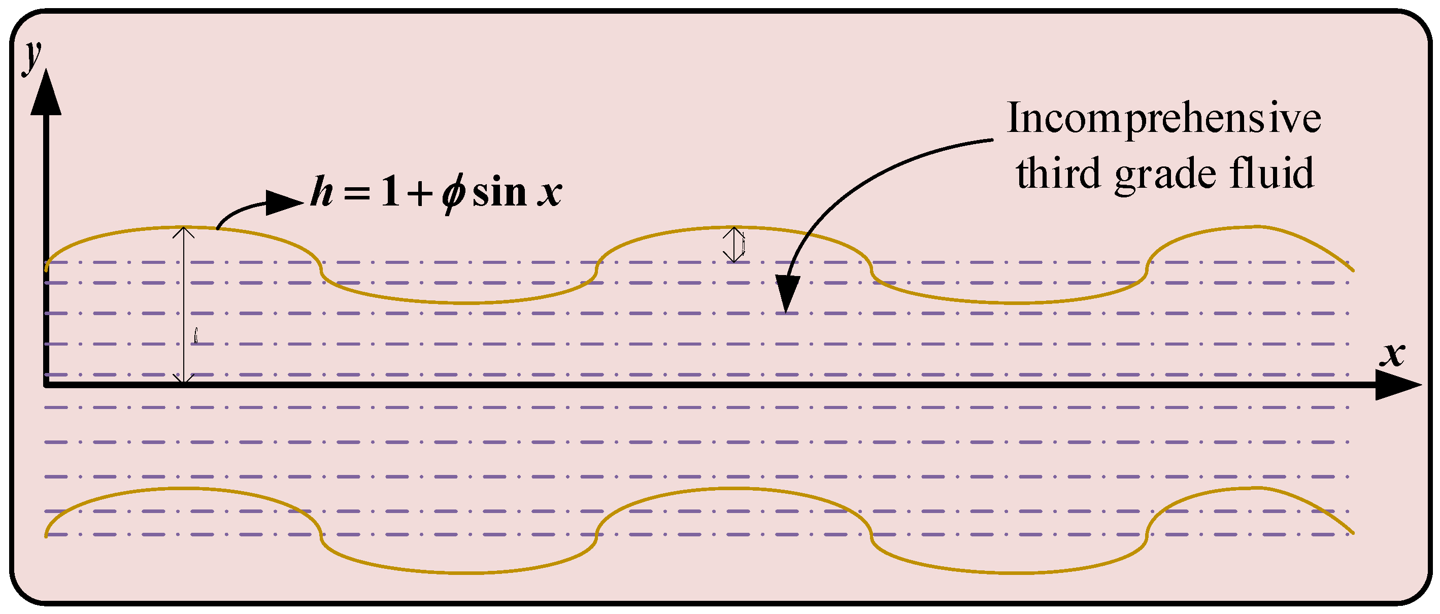
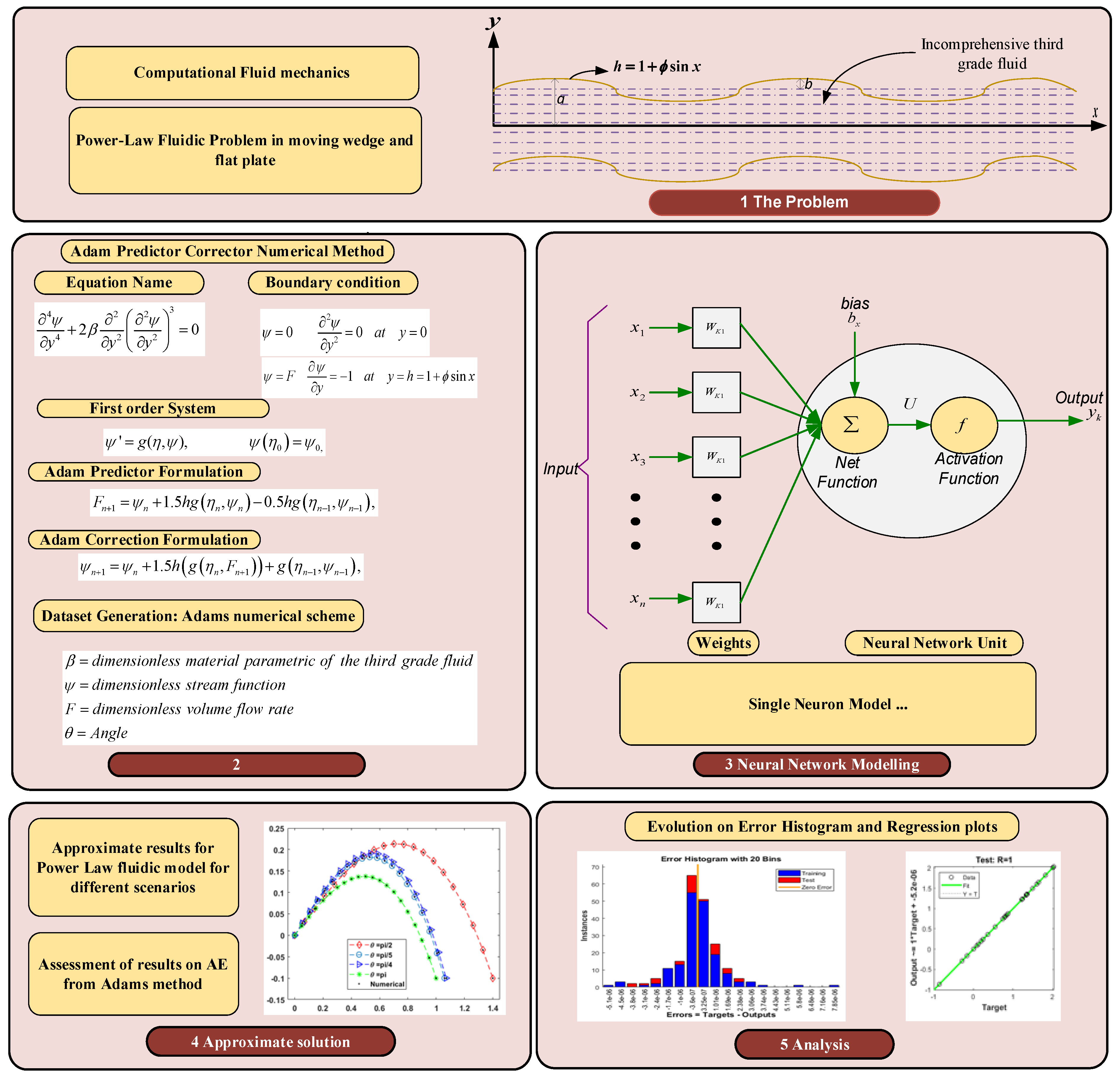
2. Problem Formulation
3. Methodology with Performance Metrics
3.1. Adams Numerical Scheme
3.2. Bayesian Regularization Neural Networks
- The execution of maximum epochs.
- The maximum set time is exceeded.
- Performance goal is attained.
- The performance gradient is less than the minimum gradient value, i.e., min_grad.
- Adaptive parameter mu is greater than its maximum value, i.e., mu_max.
3.3. Performance Measuring Metrics
4. Results and Discussion
5. Conclusions
Author Contributions
Funding
Institutional Review Board Statement
Informed Consent Statement
Conflicts of Interest
References
- Brasseur, J.G.; Corrsin, S.; Lu, N.Q. The influence of a peripheral layer of different viscosity on peristaltic pumping with Newtonian fluids. J. Fluid Mech. 1987, 174, 495–519. [Google Scholar] [CrossRef]
- Takabatake, S.; Ayukawa, K.; Mori, A. Peristaltic pumping in circular cylindrical tubes: A numerical study of fluid transport and its efficiency. J. Fluid Mech. 1988, 193, 267–283. [Google Scholar] [CrossRef]
- Prakash, J.; Sharma, A.; Tripathi, D. Thermal radiation effects on electroosmosis modulated peristaltic transport of ionic nanoliquids in biomicrofluidics channel. J. Mol. Liq. 2018, 249, 843–855. [Google Scholar]
- Sinnott, M.D.; Cleary, P.W.; Harrison, S.M. Peristaltic transport of a particulate suspension in the small intestine. Appl. Math. Model. 2017, 44, 143–159. [Google Scholar] [CrossRef]
- Hussain, S.; Ali, N. Electro-kinetically modulated peristaltic transport of multilayered power-law fluid in an axisymmetric tube. Eur. Phys. J. Plus 2020, 135, 348. [Google Scholar] [CrossRef]
- Vaidya, H.; Choudhari, R.; Gudekote, M.; Prasad, K.V. Effect of variable liquid properties on peristaltic transport of Rabinowitsch liquid in convectively heated complaint porous channel. J. Cent. South Univ. 2019, 26, 1116–1132. [Google Scholar] [CrossRef]
- Rajashekhar, C.; Manjunatha, G.; Prasad, K.V.; Divya, B.B.; Vaidya, H. Peristaltic transport of two-layered blood flow using Herschel–Bulkley Model. Cogent Eng. 2018, 5, 1495592. [Google Scholar]
- Sobhani, S.M.J.; Khabazi, N.P.; Bazargan, S.; Sadeghi, P.; Sadeghy, K. Peristaltic transport of thixotropic fluids: A numerical simulation. Korea-Aust. Rheol. J. 2019, 31, 71–79. [Google Scholar] [CrossRef]
- Saravana, R.; Vajravelu, K.; Sreenadh, S. Influence of compliant walls and heat transfer on the peristaltic transport of a Rabinowitsch fluid in an inclined channel. Z. Für Nat. A 2018, 73, 833–843. [Google Scholar] [CrossRef]
- Choudhari, R.; Gudekote, M. Slip effects on peristaltic transport of Casson fluid in an inclined elastic tube with porous walls. J. Adv. Res. Fluid Mech. Therm. Sci. 2018, 43, 67–80. [Google Scholar]
- Riaz, A. Thermal analysis of an Eyring–Powell fluid peristaltic transport in a rectangular duct with mass transfer. J. Therm. Anal. Calorim. 2020, 143, 1–13. [Google Scholar] [CrossRef]
- Tripathi, D.; Prakash, J.; Reddy, M.G.; Misra, J.C. Numerical simulation of double diffusive convection and electroosmosis during peristaltic transport of a micropolar nanofluid on an asymmetric microchannel. J. Therm. Anal. Calorim. 2020, 143, 1–16. [Google Scholar] [CrossRef]
- Nisar, Z.; Hayat, T.; Alsaedi, A.; Ahmad, B. Significance of activation energy in radiative peristaltic transport of Eyring-Powell nanofluid. Int. Commun. Heat Mass Transf. 2020, 116, 104655. [Google Scholar] [CrossRef]
- Riaz, A.A.; Al-Olayan, H.; Zeeshan, A.; Razaq, A.; Bhatti, M.M. Mass transport with asymmetric peristaltic propulsion coated with synovial fluid. Coatings 2018, 8, 407. [Google Scholar] [CrossRef] [Green Version]
- Tripathi, D.; Yadav, A.; Bég, O.A. Electro-kinetically driven peristaltic transport of viscoelastic physiological fluids through a finite length capillary: Mathematical modeling. Math. Biosci. 2017, 283, 155–168. [Google Scholar] [CrossRef]
- Zeeshan, A.; Ijaz, N.; Abbas, T.; Ellahi, R. The sustainable characteristic of bio-bi-phase flow of peristaltic transport of MHD Jeffrey fluid in the human body. Sustainability 2018, 10, 2671. [Google Scholar] [CrossRef] [Green Version]
- Tanveer, A.; Khan, M.; Salahuddin, T.; Malik, M.Y. Numerical simulation of electroosmosis regulated peristaltic transport of Bingham nanofluid. Comput. Methods Programs Biomed. 2019, 180, 105005. [Google Scholar] [CrossRef]
- Salahuddin, T.; Khan, M.H.U.; Arshad, M.; Abdel-Sattar, M.A.; Elmasry, Y. Peristaltic transport of γAl2O3/H2O and γAl2O3/C2H6O2 in an asymmetric channel. J. Mater. Res. Technol. 2020, 9, 8337–8349. [Google Scholar] [CrossRef]
- Gudekote, M.; Choudhari, R.; Vaidya, H.; Prasad, K.V. Peristaltic flow of Herschel-Bulkley fluid in an elastic tube with slip at porous walls. J. Adv. Res. Fluid Mech. Therm. Sci. 2018, 52, 63–75. [Google Scholar]
- Ramesh, K.; Prakash, J. Thermal analysis for heat transfer enhancement in electroosmosis-modulated peristaltic transport of Sutterby nanofluids in a microfluidic vessel. J. Therm. Anal. Calorim. 2019, 138, 1311–1326. [Google Scholar] [CrossRef]
- Abbas, Z.; Rafiq, M.Y.; Hasnain, J.; Umer, H. Impacts of lorentz force and chemical reaction on peristaltic transport of Jeffrey fluid in a penetrable channel with injection/suction at walls. Alex. Eng. J. 2021, 60, 1113–1122. [Google Scholar] [CrossRef]
- Eldabe, N.T.; Abouzeid, M.; Shawky, H.A. MHD Peristaltic Transport of Bingham Blood Fluid with Heat and Mass Transfer Through a Non-Uniform Channel. J. Adv. Res. Fluid Mech. Therm. Sci. 2021, 77, 145–159. [Google Scholar] [CrossRef]
- Divya, B.B.; Manjunatha, G.; Rajashekhar, C.; Vaidya, H.; Prasad, K.V. Analysis of temperature dependent properties of a peristaltic MHD flow in a non-uniform channel: A Casson fluid model. Ain Shams Eng. J. 2021, 12, 2181–2191. [Google Scholar] [CrossRef]
- Hosham, H.A.; Hafez, N.M. Bifurcation phenomena in the peristaltic transport of non-Newtonian fluid with heat and mass transfer effects. J. Appl. Math. Comput. 2021, 67, 275–299. [Google Scholar] [CrossRef]
- Javid, K.; Khan, S.U.D.; Khan, S.U.D.; Hassan, M.; Khan, A.; Alharbi, S.A. Mathematical modeling of magneto-peristaltic propulsion of a viscoelastic fluid through a complex wavy non-uniform channel: An application of hall device in bio-engineering domains. Eur. Phys. J. Plus 2021, 136, 1–31. [Google Scholar]
- Vaidya, H.; Rajashekhar, C.; Prasad, K.V. Heat transfer and Slip Consequences on Peristaltic Transport of a Casson Fluid in an Asymmetric Porous Channel. J. Porous Media 2021, 24, 77–94. [Google Scholar] [CrossRef]
- Waseem, W.; Sulaiman, M.; Islam, S.; Kumam, P.; Nawaz, R.; Raja, M.A.Z.; Farooq, M.; Shoaib, M. A study of changes in temperature profile of porous fin model using cuckoo search algorithm. Alex. Eng. J. 2020, 59, 11–24. [Google Scholar] [CrossRef]
- Zúñiga-Aguilar, C.J.; Romero-Ugalde, H.M.; Gómez-Aguilar, J.F.; Escobar-Jiménez, R.F.; Valtierra-Rodríguez, M. Solving fractional differential equations of variable-order involving operators with Mittag-Leffler kernel using artificial neural networks. Chaos Solitons Fractals 2017, 103, 382–403. [Google Scholar] [CrossRef]
- Bukhari, A.H.; Sulaiman, M.; Islam, S.; Shoaib, M.; Kumam, P.; Raja, M.A.Z. Neuro-fuzzy modeling and prediction of summer precipitation with application to different meteorological stations. Alex. Eng. J. 2020, 59, 101–116. [Google Scholar] [CrossRef]
- Jafarian, A.; Mokhtarpour, M.; Baleanu, D. Artificial neural network approach for a class of fractional ordinary differential equation. Neural Comput. Appl. 2017, 28, 765–773. [Google Scholar] [CrossRef]
- Raja, M.A.Z. Stochastic numerical treatment for solving Troesch’s problem. Inf. Sci. 2014, 279, 860–873. [Google Scholar] [CrossRef]
- Mehmood, A.; Zameer, A.; Aslam, M.S.; Raja, M.A.Z. Design of nature-inspired heuristic paradigm for systems in nonlinear electrical circuits. Neural Comput. Appl. 2020, 32, 7121–7137. [Google Scholar] [CrossRef]
- Raja, M.A.Z.; Mehmood, A.; Niazi, S.A.; Shah, S.M. Computational intelligence methodology for the analysis of RC circuit modelled with nonlinear differential order system. Neural Comput. Appl. 2018, 30, 1905–1924. [Google Scholar] [CrossRef]
- Sabir, Z.; Raja, M.A.Z.; Guirao, J.L.; Shoaib, M. A novel design of fractional Meyer wavelet neural networks with application to the nonlinear singular fractional Lane-Emden systems. Alex. Eng. J. 2021, 60, 2641–2659. [Google Scholar] [CrossRef]
- Ahmad, I.; Ahmad, S.; Awais, M.; Ahmad, S.U.I.; Raja, M.A.Z. Neuro-evolutionary computing paradigm for Painlevé equation-II in nonlinear optics. Eur. Phys. J. Plus 2018, 133, 184. [Google Scholar] [CrossRef]
- Jadoon, I.; Raja, M.A.Z.; Junaid, M.; Ahmed, A.; ur Rehman, A.; Shoaib, M. Design of evolutionary optimized finite difference based numerical computing for dust density model of nonlinear Van-der Pol Mathieu’s oscillatory systems. Math. Comput. Simul. 2021, 181, 444–470. [Google Scholar] [CrossRef]
- Raja, M.A.Z.; Mehmood, A.; Khan, A.A.; Zameer, A. Integrated intelligent computing for heat transfer and thermal radiation-based two-phase MHD nanofluid flow model. Neural Comput. Appl. 2020, 32, 2845–2877. [Google Scholar] [CrossRef]
- Mehmood, A.; Zameer, A.; Ling, S.H.; Raja, M.A.Z. Design of neuro-computing paradigms for nonlinear nanofluidic systems of MHD Jeffery–Hamel flow. J. Taiwan Inst. Chem. Eng. 2018, 91, 57–85. [Google Scholar] [CrossRef]
- Shah, Z.; Raja, M.A.Z.; Chu, Y.M.; Khan, W.A.; Abbas, S.Z.; Shoaib, M.; Irfan, M. Computational intelligence of Levenberg-Marquardt backpropagation neural networks to study the dynamics of expanding/contracting cylinder for Cross magneto-nanofluid flow model. Phys. Scr. 2021, 96, 055219. [Google Scholar] [CrossRef]
- Mehmood, A.; Zameer, A.; Raja, M.A.Z. Intelligent computing to analyze the dynamics of magnetohydrodynamic flow over stretchable rotating disk model. Appl. Soft Comput. 2018, 67, 8–28. [Google Scholar] [CrossRef]
- Shoaib, M.; Raja, M.A.Z.; Sabir, M.T.; Bukhari, A.H.; Alrabaiah, H.; Shah, Z.; Kumam, P.; Islam, S. A Stochastic Numerical Analysis Based on Hybrid NAR-RBFs Networks Nonlinear SITR Model for Novel COVID-19 Dynamics. Comput. Methods Programs Biomed. 2021, 202, 105973. [Google Scholar] [CrossRef]
- Sabir, Z.; Raja, M.A.Z.; Umar, M.; Shoaib, M. Design of neuro-swarming-based heuristics to solve the third-order nonlinear multi-singular Emden–Fowler equation. Eur. Phys. J. Plus 2020, 135, 410. [Google Scholar] [CrossRef]
- Sabir, Z.; Manzar, M.A.; Raja, M.A.Z.; Sheraz, M.; Wazwaz, A.M. Neuro-heuristics for nonlinear singular Thomas-Fermi systems. Appl. Soft Comput. 2018, 65, 152–169. [Google Scholar] [CrossRef]
- Sabir, Z.; Khalique, C.M.; Raja, M.A.Z.; Baleanu, D. Evolutionary computing for nonlinear singular boundary value problems using neural network, genetic algorithm and active-set algorithm. Eur. Phys. J. Plus 2021, 136, 1–19. [Google Scholar] [CrossRef]
- Raja, M.A.Z.; Shah, Z.; Manzar, M.A.; Ahmad, I.; Awais, M.; Baleanu, D. A new stochastic computing paradigm for nonlinear Painlevé II systems in applications of random matrix theory. Eur. Phys. J. Plus 2018, 133, 254. [Google Scholar] [CrossRef]
- Khan, J.A.; Raja, M.A.Z.; Rashidi, M.M.; Syam, M.I.; Wazwaz, A.M. Nature-inspired computing approach for solving non-linear singular Emden–Fowler problem arising in electromagnetic theory. Connect. Sci. 2015, 27, 377–396. [Google Scholar] [CrossRef]
- Akbar, S.; Zaman, F.; Asif, M.; Rehman, A.U.; Raja, M.A.Z. Novel application of FO-DPSO for 2-D parameter estimation of electromagnetic plane waves. Neural Comput. Appl. 2019, 31, 3681–3690. [Google Scholar] [CrossRef]
- Umar, M.; Sabir, Z.; Amin, F.; Guirao, J.L.G.; Raja, M.A.Z. Stochastic numerical technique for solving HIV infection model of CD4+ T cells. Eur. Phys. J. Plus 2020, 135, 1–19. [Google Scholar] [CrossRef]
- Umar, M.; Sabir, Z.; Raja, M.A.Z.; Amin, F.; Saeed, T.; Guerrero-Sanchez, Y. Integrated neuro-swarm heuristic with interior-point for nonlinear SITR model for dynamics of novel COVID-19. Alex. Eng. J. 2021, 60, 2811–2824. [Google Scholar] [CrossRef]
- Bukhari, H.; Raja, M.A.Z.; Sulaiman, M.; Islam, S.; Shoaib, M.; Kumam, P. Fractional neuro-sequential ARFIMA-LSTM for financial market forecasting. IEEE Access 2020, 8, 71326–71338. [Google Scholar] [CrossRef]
- Ara, A.; Khan, N.A.; Razzaq, O.A.; Hameed, T.; Raja, M.A.Z. Wavelets optimization method for evaluation of fractional partial differential equations: An application to financial modelling. Adv. Differ. Equ. 2018, 2018, 8. [Google Scholar] [CrossRef]
- Raja, M.A.Z.; Manzar, M.A.; Shah, S.M.; Chen, Y. Integrated intelligence of fractional neural networks and sequential quadratic programming for Bagley–Torvik systems arising in fluid mechanics. J. Comput. Nonlinear Dyn. 2020, 15, 051003. [Google Scholar] [CrossRef]
- Lodhi, S.; Manzar, M.A.; Raja, M.A.Z. Fractional neural network models for nonlinear Riccati systems. Neural Comput. Appl. 2019, 31, 359–378. [Google Scholar] [CrossRef]
- Sabir, Z.; Raja, M.A.Z.; Shoaib, M.; Aguilar, J.G. FMNEICS: Fractional Meyer neuro-evolution-based intelligent computing solver for doubly singular multi-fractional order Lane–Emden system. Comput. Appl. Math. 2020, 39, 1–18. [Google Scholar] [CrossRef]
- Burden, F.; Winkler, D. Bayesian regularization of neural networks. Artif. Neural Netw. 2008, 458, 23–42. [Google Scholar]
- Hirschen, K.; Schäfer, M. Bayesian regularization neural networks for optimizing fluid flow processes. Comput. Methods Appl. Mech. Eng. 2006, 195, 481–500. [Google Scholar] [CrossRef]
- Shi, J.; Zhu, Y.; Khan, F.; Chen, G. Application of Bayesian Regularization Artificial Neural Network in explosion risk analysis of fixed offshore platform. J. Loss Prev. Process Ind. 2019, 57, 131–141. [Google Scholar] [CrossRef]
- Soltanali, H.; Khojastehpour, M.; Farinha, J.T. An Integrated Fuzzy Fault Tree Model with Bayesian Network-Based Maintenance Optimization of Complex Equipment in Automotive Manufacturing. Energies 2021, 14, 7758. [Google Scholar] [CrossRef]
- Awan, S.E.; Raja, M.A.Z.; Awais, M.; Shu, C.M. Intelligent Bayesian regularization networks for bio-convective nanofluid flow model involving gyro-tactic organisms with viscous dissipation, stratification and heat immersion. Eng. Appl. Comput. Fluid Mech. 2021, 15, 1508–1530. [Google Scholar] [CrossRef]
- Hayat, T.; Wang, Y.; Siddiqui, A.M.; Hutter, K.; Asghar, S. Peristaltic transport of a third-order fluid in a circular cylindrical tube. Math. Models Methods Appl. Sci. 2002, 12, 1691–1706. [Google Scholar] [CrossRef]
- Hayat, T.; Khan, M.; Siddiqui, A.M.; Asghar, S. Non-linear peristaltic flow of a non-Newtonian fluid under effect of a magnetic field in a planar channel. Commun. Nonlinear Sci. Numer. Simul. 2007, 12, 910–919. [Google Scholar] [CrossRef]
- Ashraf, H.; Siddiqui, A.M.; Rana, M.A. Fallopian tube analysis of the peristaltic-ciliary flow of third grade fluid in a finite narrow tube. Chin. J. Phys. 2018, 56, 605–621. [Google Scholar] [CrossRef]
- MacKay, D.J. Bayesian interpolation. Neural Comput. 1992, 4, 415–447. [Google Scholar] [CrossRef]
- Awan, S.E.; Raja, M.A.Z.; Gul, F.; Khan, Z.A.; Mehmood, A.; Shoaib, M. Numerical Computing Paradigm for Investigation of Micropolar Nanofluid Flow Between Parallel Plates System with Impact of Electrical MHD and Hall Current. Arab. J. Sci. Eng. 2021, 46, 645–662. [Google Scholar] [CrossRef]
- Chaudhary, N.I.; Manzar, M.A.; Raja, M.A.Z. Fractional Volterra LMS algorithm with application to Hammerstein control autoregressive model identification. Neural Comput. Appl. 2019, 31, 5227–5240. [Google Scholar] [CrossRef]
- Chaudhary, N.I.; Zubair, S.; Aslam, M.S.; Raja, M.A.Z.; Machado, J.T. Design of momentum fractional LMS for Hammerstein nonlinear system identification with application to electrically stimulated muscle model. Eur. Phys. J. Plus 2019, 134, 1–15. [Google Scholar] [CrossRef]
- Masood, Z.; Samar, R.; Raja, M.A.Z. Design of fractional order epidemic model for future generation tiny hardware implants. Future Gener. Comput. Syst. 2020, 106, 43–54. [Google Scholar] [CrossRef]
- Masood, Z.; Samar, R.; Raja, M.A.Z. Design of a mathematical model for the Stuxnet virus in a network of critical control infrastructure. Comput. Secur. 2019, 87, 101565. [Google Scholar] [CrossRef]
- Ilyas, H.; Ahmad, I.; Raja, M.A.Z.; Shoaib, M. A novel design of Gaussian WaveNets for rotational hybrid nanofluidic flow over a stretching sheet involving thermal radiation. Int. Commun. Heat Mass Transf. 2021, 123, 105196. [Google Scholar] [CrossRef]
- Shoaib, M.; Raja, M.A.Z.; Sabir, M.T.; Islam, S.; Shah, Z.; Kumam, P.; Alrabaiah, H. Numerical investigation for rotating flow of MHD hybrid nanofluid with thermal radiation over a stretching sheet. Sci. Rep. 2020, 10, 1–15. [Google Scholar] [CrossRef]


| Scenario | Case | β | θ | ϕ | F |
|---|---|---|---|---|---|
| 1 | 1 | 0.08 | π/2 | 0.4 | −0.1 |
| 2 | 0.07 | π/2 | 0.4 | −0.1 | |
| 3 | 0.04 | π/2 | 0.4 | −0.1 | |
| 4 | 0.02 | π/2 | 0.4 | −0.1 | |
| 2 | 2 | 0.08 | π/5 | 0.4 | −0.1 |
| 3 | 0.08 | π/4 | 0.4 | −0.1 | |
| 4 | 0.08 | π | 0.4 | −0.1 | |
| 3 | 2 | 0.08 | π/2 | 0.1 | −0.1 |
| 3 | 0.08 | π/2 | 0.6 | −0.1 | |
| 4 | 0.08 | π/2 | 0.7 | −0.1 | |
| 4 | 2 | 0.08 | π/2 | 0.4 | 1.2 |
| 3 | 0.08 | π/2 | 0.4 | 1.4 | |
| 4 | 0.08 | π/2 | 0.4 | 2.0 |
| Index | Settings |
|---|---|
| Maximum epochs for training | 1000 |
| Performance/fitness goal | 0 |
| Marquardt adjustment parameter, i.e., mu | 0.005 |
| Decreeing factor of mu, i.e., mu_dec | 0.1 |
| Increasing factor of mu i.e., mu_inc | 10 |
| Maximum of mu | 1010 |
| Maximum number of validation failures | Inf |
| Minimum value of performance gradient | 10−7 |
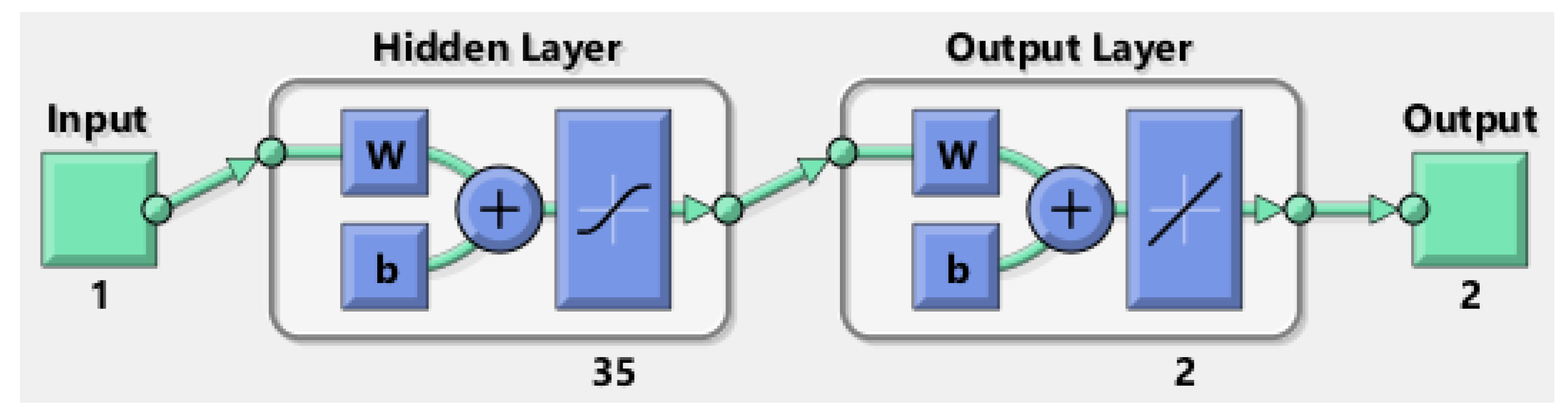
| Number of hidden neurons | 35 |
| Training and testing samples | 80 and 20 percentage |
| Sample selection | Randomize |
| Input, output, and hidden layers | Single for all three |
| Reference data set generation | Adams method |
| Scenario | Case | C | Performance Attained | Gradient Value | Mu Step Size | Epoch Executed | Consumed Time | |
|---|---|---|---|---|---|---|---|---|
| Training | Testing | |||||||
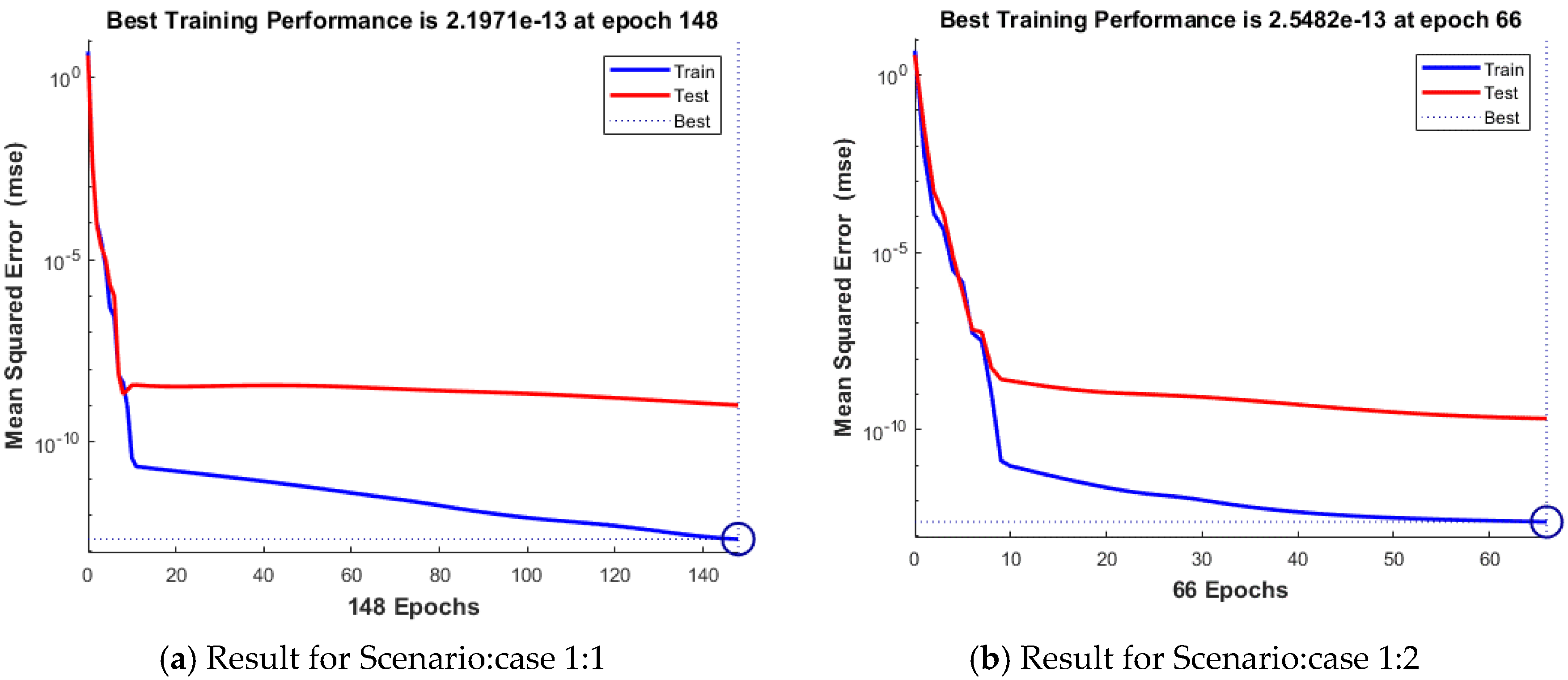
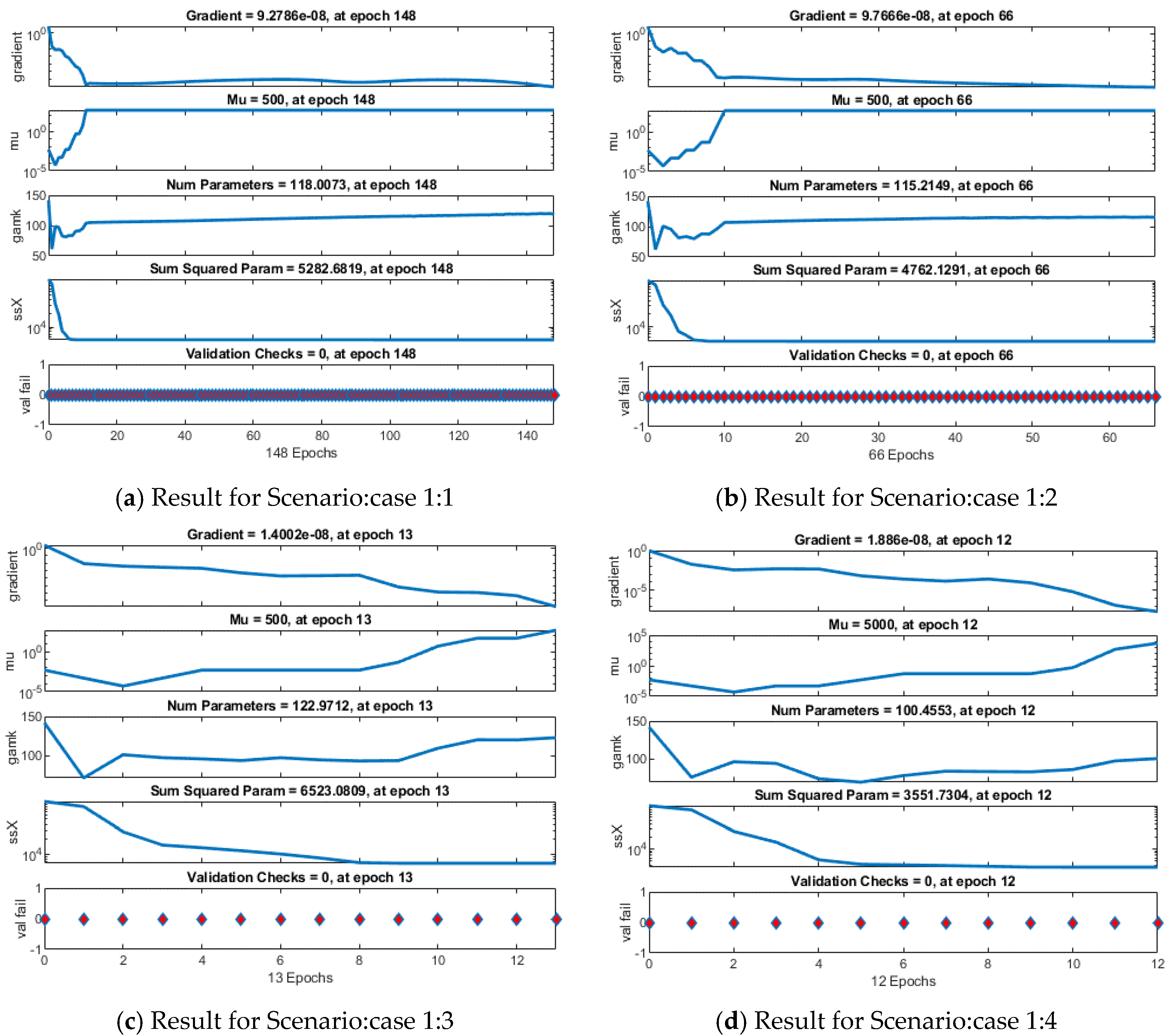
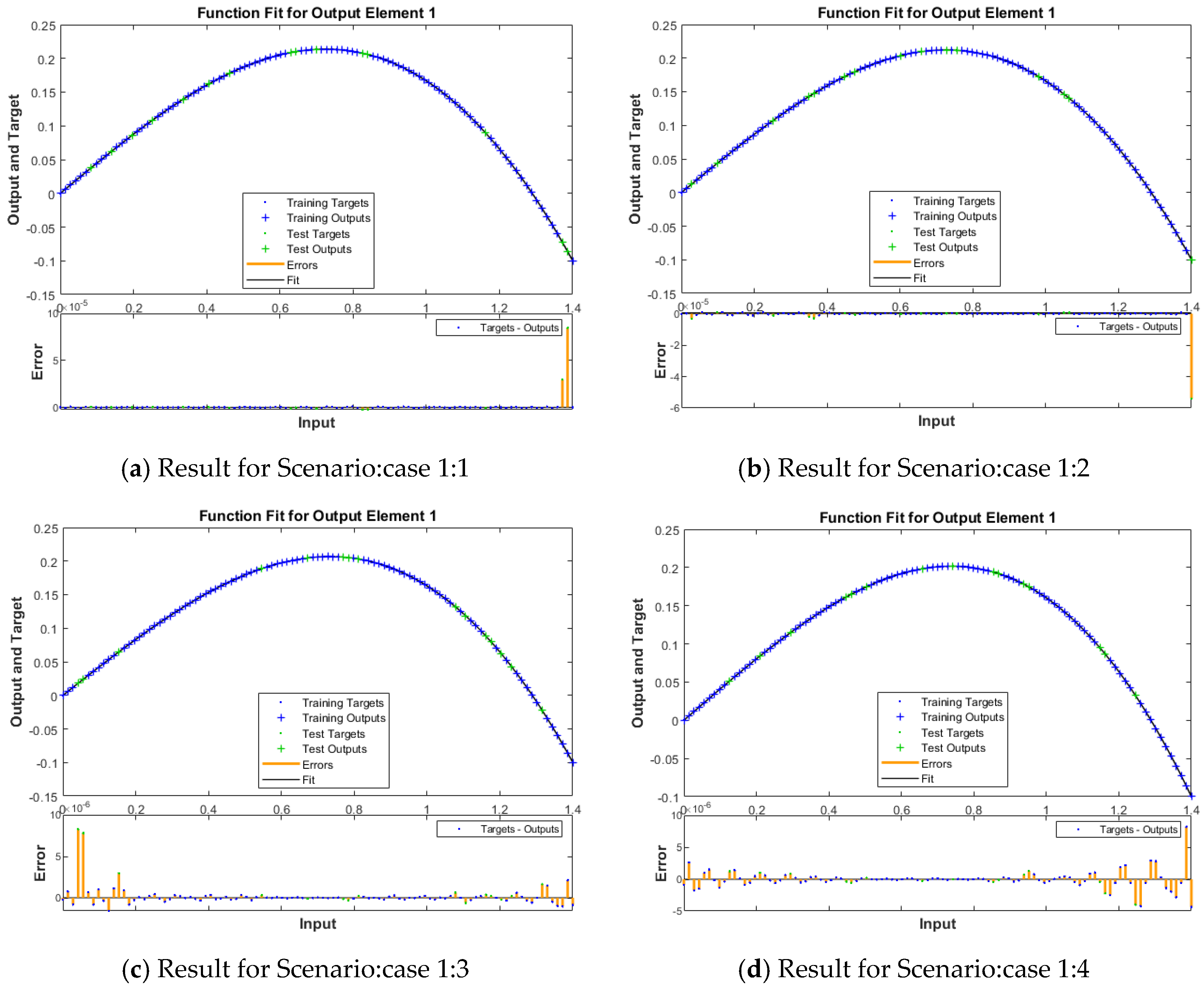
| 1 | 1 | 2.00 × 10⁻¹³ | 1.03 × 10⁻⁹ | 2.20 × 10⁻¹³ | 9.28 × 10⁻⁸ | 5.00 | 148 | 0.00.06 |
| 2 | 2.55 × 10⁻¹³ | 2.07 × 10⁻¹⁰ | 2.55 × 10⁻¹³ | 9.77 × 10⁻⁸ | 5.00 | 66 | 0.00.02 | |
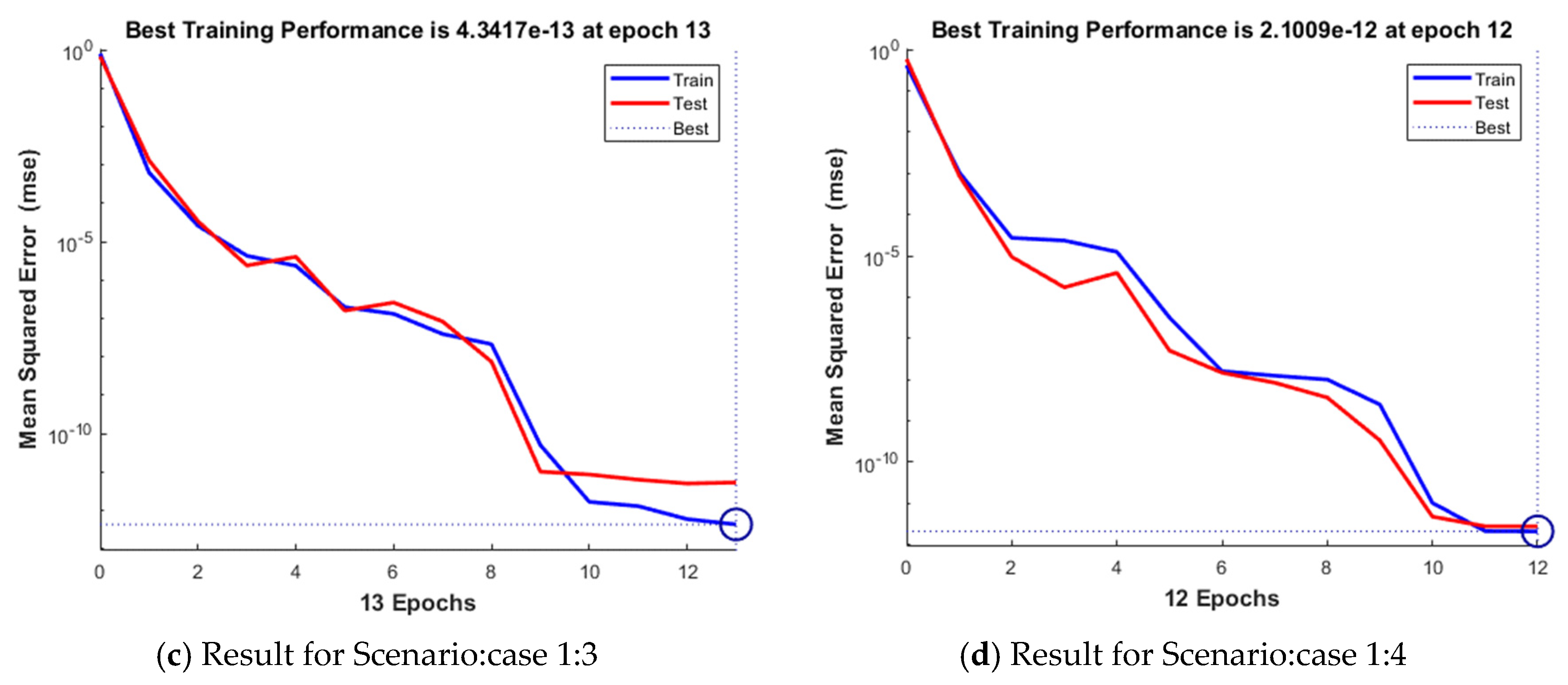
| 3 | 4.34 × 10⁻¹³ | 5.37 × 10⁻¹² | 4.34 × 10⁻¹³ | 1.40 × 10⁻⁸ | 5.00 | 13 | 0.00.01 | |
| 4 | 2.10 × 10⁻¹² | 2.77 × 10⁻⁹ | 2.10 × 10⁻¹² | 1.89 × 10⁻⁸ | 500 | 12 | 0.00.01 | |
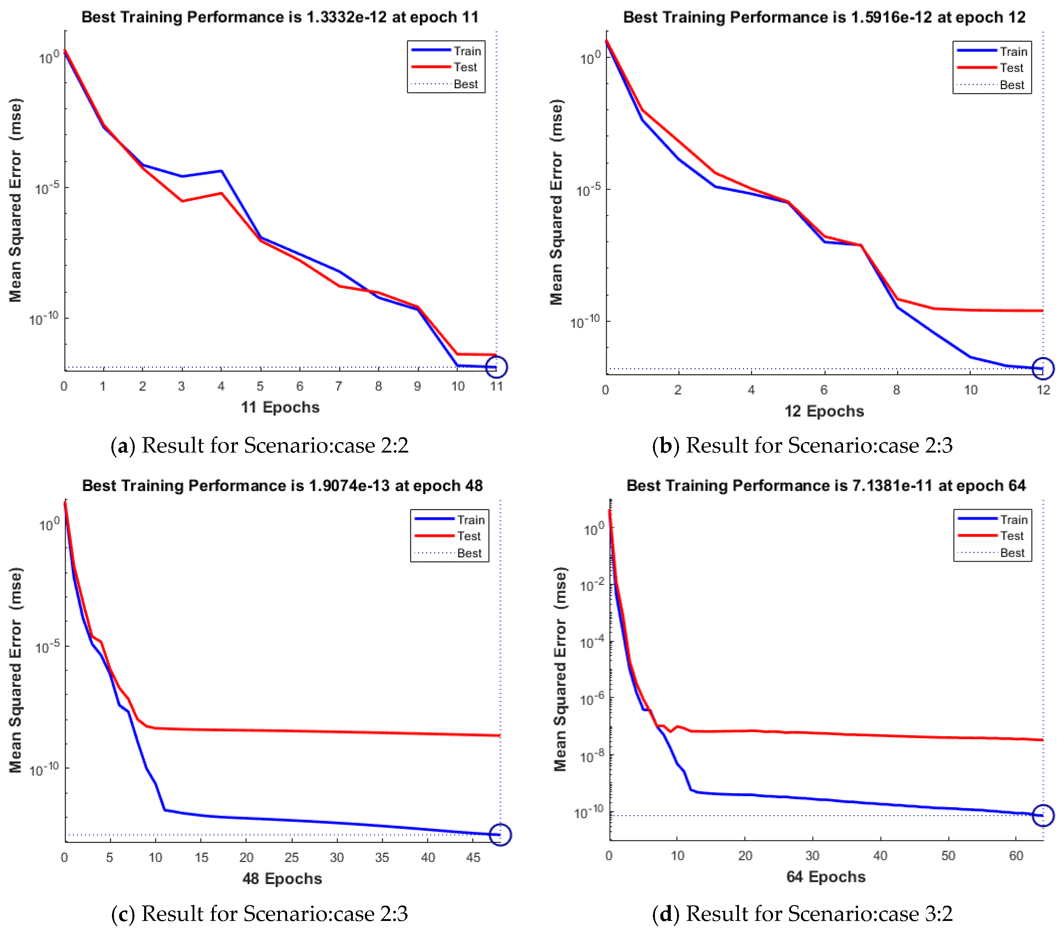
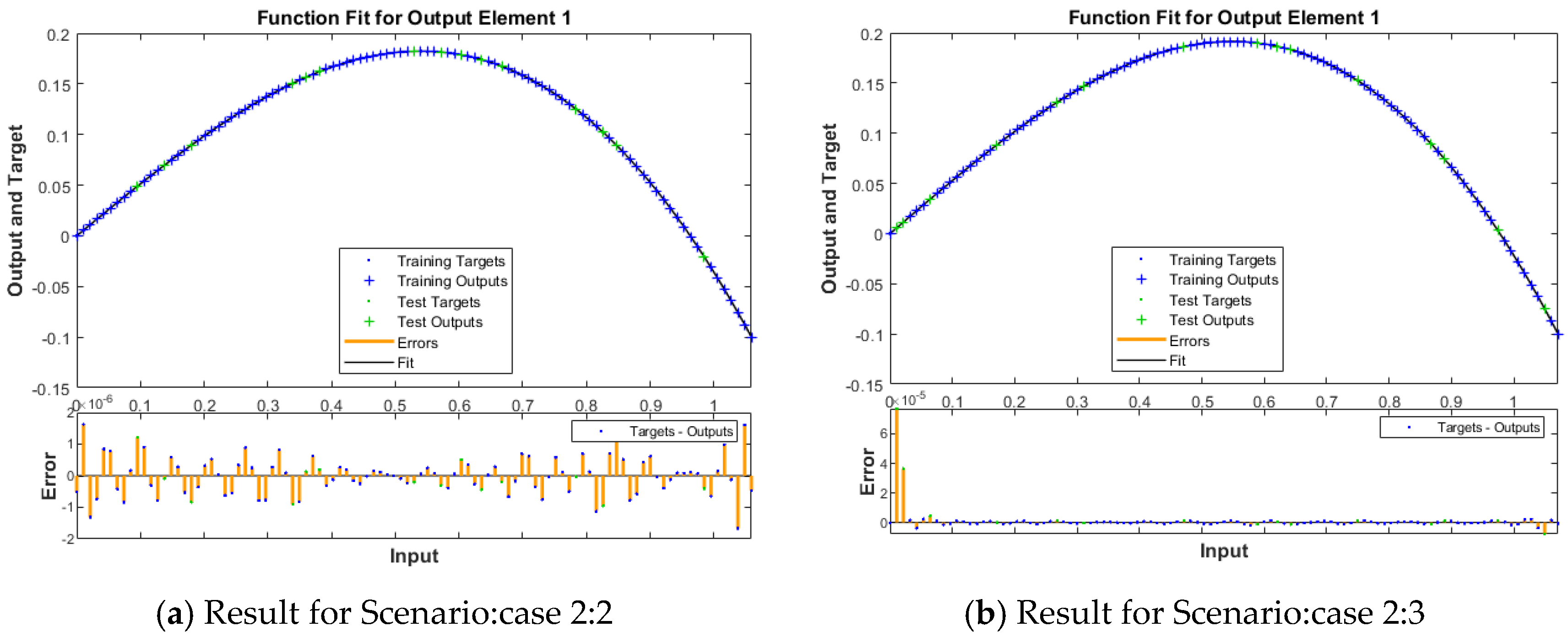
| 2 | 2 | 1.33 × 10⁻¹² | 3.98 × 10⁻¹² | 1.33 × 10⁻¹² | 1.40 × 10⁻⁸ | 500 | 11 | 0.00.01 |
| 3 | 1.59 × 10⁻¹² | 2.50 × 10⁻¹⁰ | 1.59 × 10⁻¹² | 3.82 × 10⁻⁸ | 500 | 12 | 0.00.01 | |
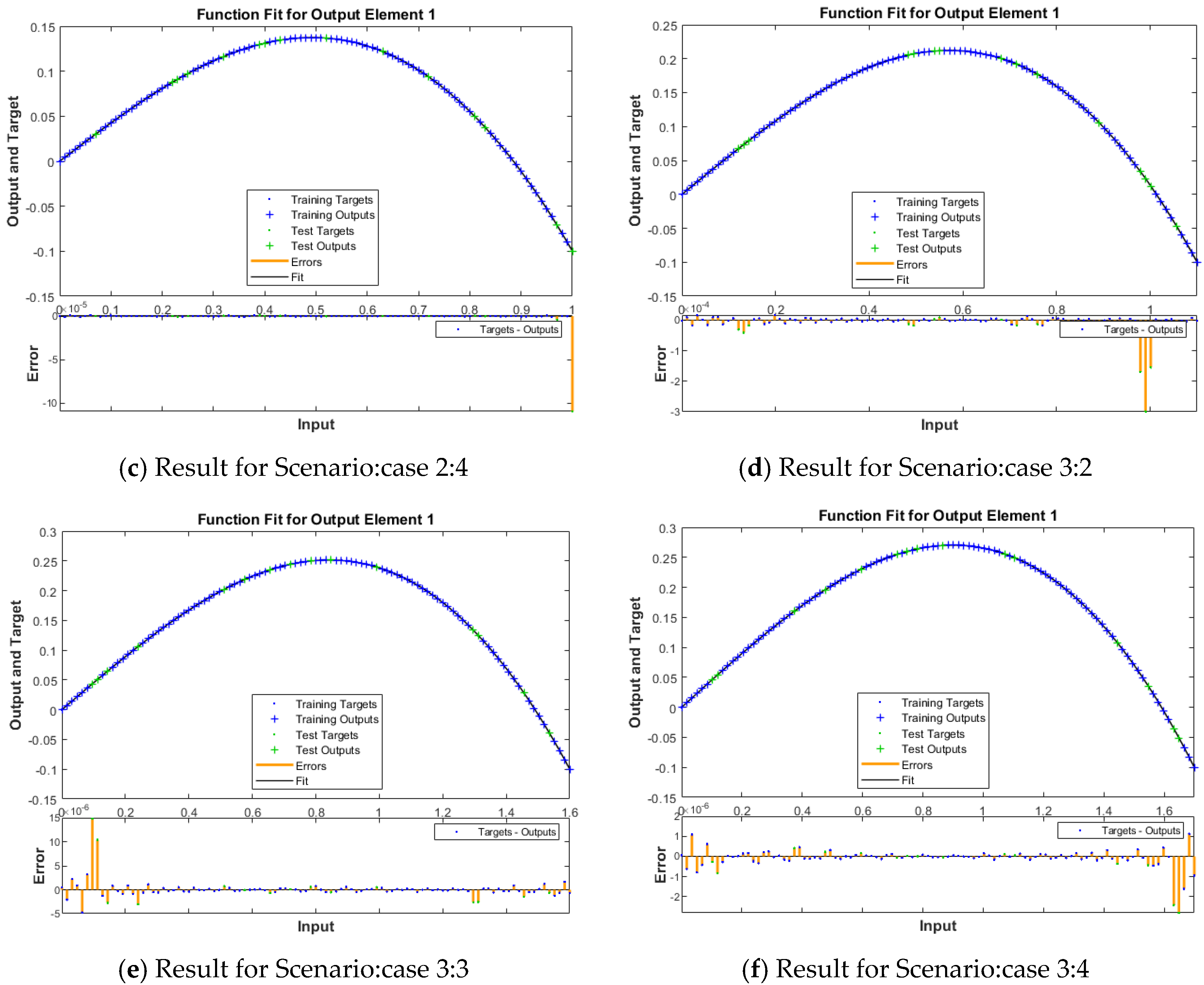
| 4 | 1.91 × 10⁻¹³ | 2.19 × 10⁻⁹ | 1.91 × 10⁻¹³ | 9.95 × 10⁻⁸ | 500 | 48 | 0.00.02 | |
| 3 | 2 | 7.14 × 10⁻¹¹ | 3.32 × 10⁻⁶ | 7.14 × 10⁻¹¹ | 5.23 × 10⁻⁸ | 500 | 64 | 0.00.02 |
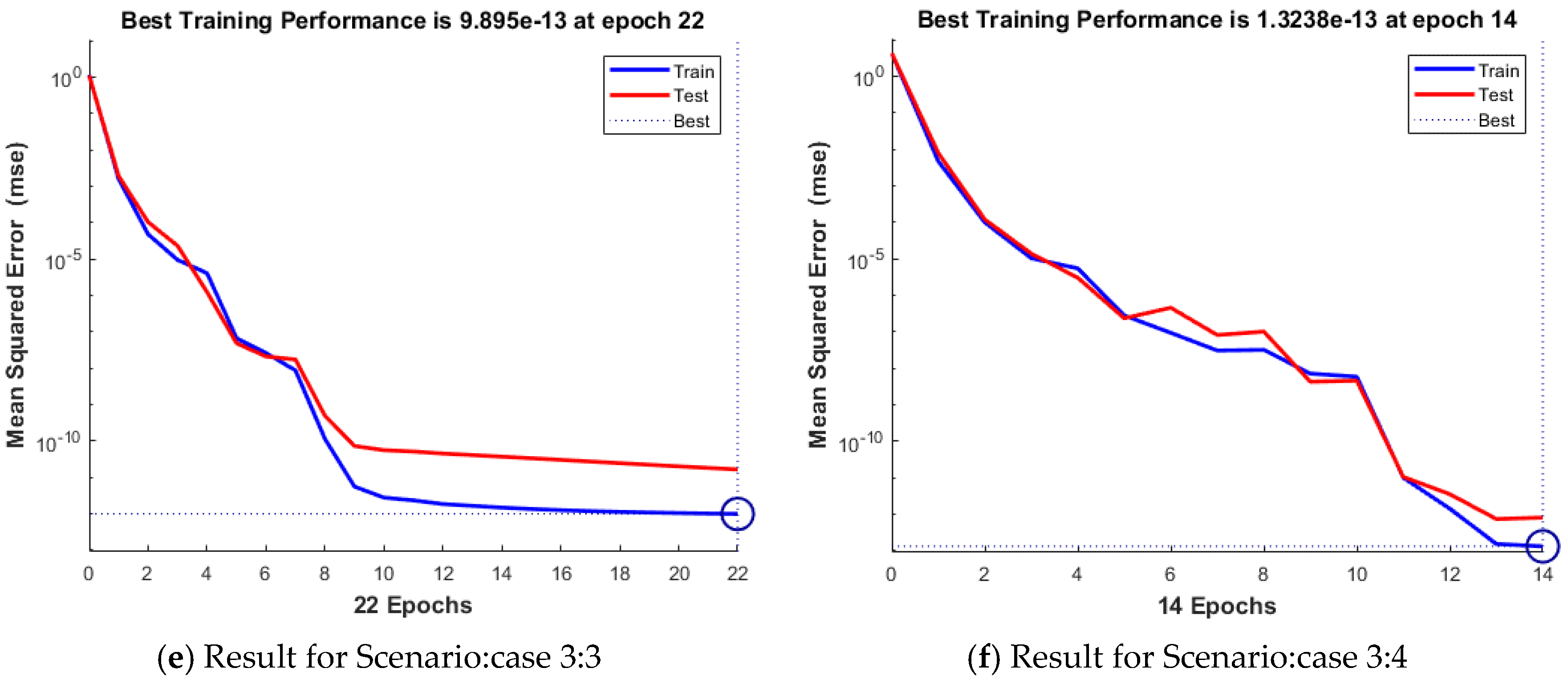
| 3 | 9.90 × 10⁻¹³ | 1.65 × 10⁻¹¹ | 9.89 × 10⁻¹³ | 9.80 × 10⁻⁸ | 500 | 22 | 0.00.01 | |
| 4 | 1.32 × 10⁻¹³ | 8.14 × 10⁻¹³ | 1.32 × 10⁻¹³ | 8.19 × 10⁻⁸ | 500 | 14 | 0.00.01 | |
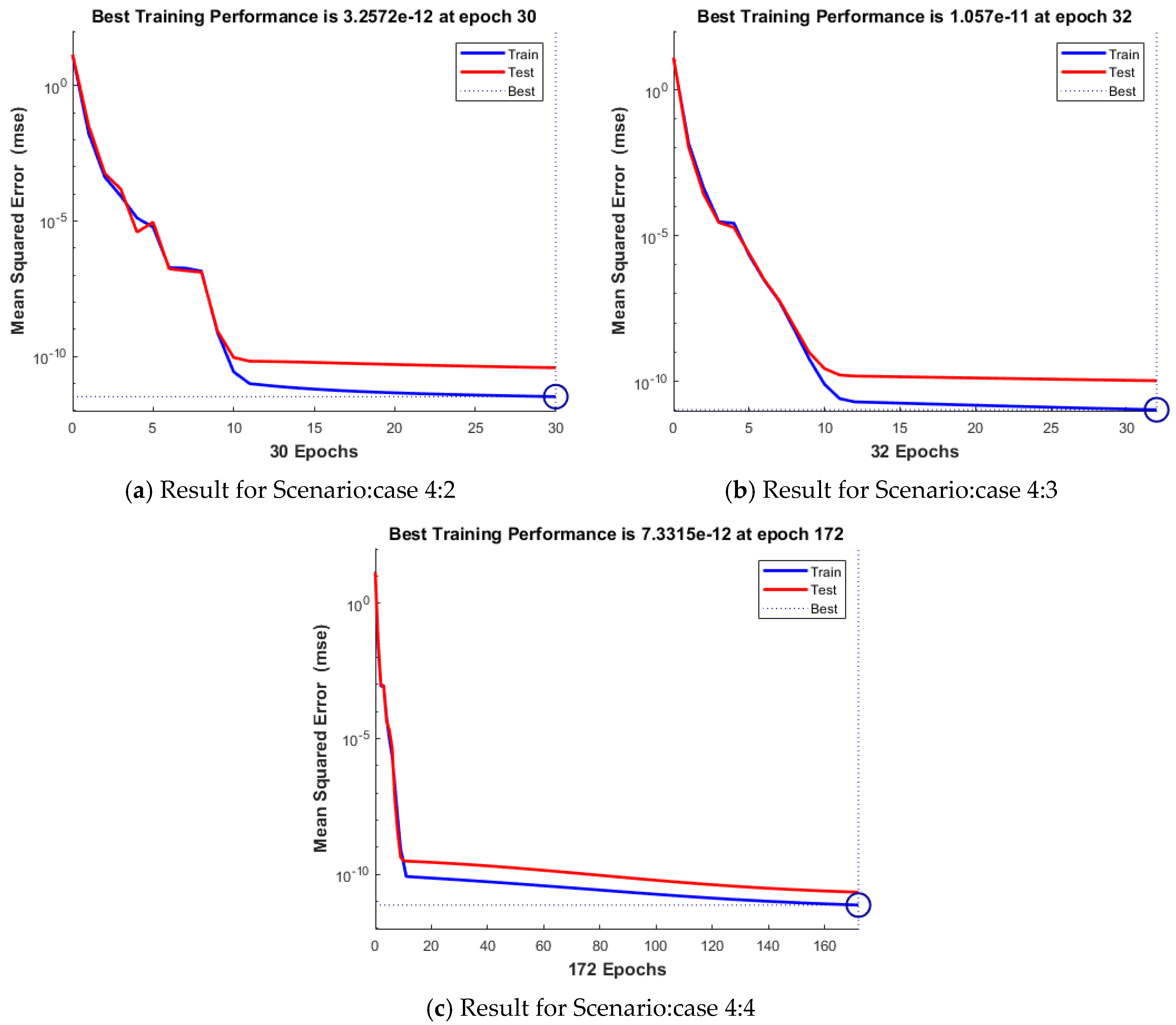
| 4 | 2 | 3.26 × 10⁻¹² | 3.82 × 10⁻¹¹ | 3.26 × 10⁻¹² | 9.94 × 10⁻⁸ | 50 | 30 | 0.00.01 |
| 3 | 1.06 × 10⁻¹¹ | 1.05 × 10⁻¹⁰ | 1.06 × 10⁻¹¹ | 9.84 × 10⁻⁸ | 50 | 32 | 0.00.01 | |
| 4 | 7.33 × 10⁻¹² | 2.18 × 10⁻¹¹ | 7.33 × 10⁻¹² | 9.81 × 10⁻⁸ | 50 | 172 | 0.00.04 | |
Publisher’s Note: MDPI stays neutral with regard to jurisdictional claims in published maps and institutional affiliations. |
© 2022 by the authors. Licensee MDPI, Basel, Switzerland. This article is an open access article distributed under the terms and conditions of the Creative Commons Attribution (CC BY) license (https://creativecommons.org/licenses/by/4.0/).
Share and Cite
Mahmood, T.; Ali, N.; Chaudhary, N.I.; Cheema, K.M.; Milyani, A.H.; Raja, M.A.Z. Novel Adaptive Bayesian Regularization Networks for Peristaltic Motion of a Third-Grade Fluid in a Planar Channel. Mathematics 2022, 10, 358. https://doi.org/10.3390/math10030358
Mahmood T, Ali N, Chaudhary NI, Cheema KM, Milyani AH, Raja MAZ. Novel Adaptive Bayesian Regularization Networks for Peristaltic Motion of a Third-Grade Fluid in a Planar Channel. Mathematics. 2022; 10(3):358. https://doi.org/10.3390/math10030358
Chicago/Turabian StyleMahmood, Tariq, Nasir Ali, Naveed Ishtiaq Chaudhary, Khalid Mehmood Cheema, Ahmad H. Milyani, and Muhammad Asif Zahoor Raja. 2022. "Novel Adaptive Bayesian Regularization Networks for Peristaltic Motion of a Third-Grade Fluid in a Planar Channel" Mathematics 10, no. 3: 358. https://doi.org/10.3390/math10030358
APA StyleMahmood, T., Ali, N., Chaudhary, N. I., Cheema, K. M., Milyani, A. H., & Raja, M. A. Z. (2022). Novel Adaptive Bayesian Regularization Networks for Peristaltic Motion of a Third-Grade Fluid in a Planar Channel. Mathematics, 10(3), 358. https://doi.org/10.3390/math10030358