Experimental Validation of Model Heat Transfer in Rectangular Hole Beams Using Modern Dimensional Analysis

Abstract

Based on the Szirtes’ modern dimensional analysis (MDA), the authors apply the theory to a real structure in order to validate by experimental measurements its applicability. After a presentation of the basic elements of the model law (ML), deduced for two relevant cases, the authors conceived the set of prototypes and models, based on the case of an actual construction pillar, physically performed at scales of 1:1, 1:2, and 1:4. The combination of these structural elements, made at different scales, resulted in three sets of prototypes and models. In this paper, taking into consideration the ML for two relevant cases, the following are presented: the original test stand of these structural elements; block diagram of the original electronic heating and control system; the basic considerations regarding the particularity of this heating system from the point of view of heat transfer; measurement data, obtained for both nonthermally protected elements and for those protected with layers of intumescent paints. In the last part of the paper, the values obtained by rigorous direct measurements with those offered by the ML on the elements considered as prototypes and models are compared. Almost identical values were obtained from the direct measurements with those provided by the ML, thus resulting in the validation of these laws. The same thermal regimes were applied to all these structural elements, with registration of every parameter related to these thermal regimes. Depending on the role of a structural element within a certain set (prototype-model), some of the measurement data were considered as data acquired directly through measurements, and others served as reference elements for those for which we had to obtain through the model law. In the last part of the paper, the sizes obtained by rigorous direct measurements are compared with those offered by the model law on the elements considered as prototypes and models. Identical practical values of the quantities were obtained from the direct measurements with those provided by the model law, thus resulting in the validation of these laws.

1. Introduction

A number of methods have been developed to protect metal structures from fire. In general, protections fall into two broad groups: passive and active. Metal structures can be protected with different passive methods:

• Protection with fire-resistant boards (e.g., gypsum board, calcium silicate boards);
• Cover with flexible blanket (from different materials);
• Shot blasting products:

  ○

  Dry mortar coating: cement-based or sulfide-based;

  ○

  Cementites/vermiculite spray

  ○

  Mortar composed of vermiculite and plaster;

  ○

  Mortar based on mineral flax, addition of cement, bentonite, and other additives;

• Concrete coating of steel profiles;
• Protection with intumescent paint;
• Tile dressing.

Regardless of the material of the structure to be protected or the method of protection used against fire, the purpose is to prevent the temperature of the covered structure from rising in order to maintain its integrity and stability.

The issue of assessing the quality of the thermal insulation/thermal protection of the various solutions as accurately as possible is a very topical and important issue, both in terms of the protection of human lives and the material goods. In this regard, increasingly more accurate calculations have been developed to predict the load-bearing capacity of fire-resistant structures. The authors’ current concerns regarding dimensional analysis fall in this direction, and we hope that the results presented below will be useful to engineers and researchers in the field.

Dimensional analysis began to be perceived as a tool of analysis in physics in the late eighteenth century. This method emerged as a result of the introduction of fundamental units for characterizing the fundamental quantities with which science began to operate [1].

The method proved to be simple and, especially for this, it was accepted in section XIX and XX for the investigation of complex structures. In essence, the method consists of executing/manufacturing a model at a certain scale of the real structure and the experimental investigation of this model. Based on the results obtained experimentally, on the model, one can obtain by means of ML the expected results for the real structure. Thus, the experimental results obtained on the model built in the laboratory can be extrapolated to obtain the results sought for the real structure, applying the so-called law of the model, constituted from a finite number of dimensionless variables starting from Buckingham’s theorem [2].

The MDA method, which was applied here, offers us a model law, unique for the phenomenon studied. The method is based on the exclusion of irrelevant physical variables. In this way, a model law is obtained that describes the correlation between the model and the prototype made on a certain scale. The applicability limits are presented in [3,4]. The method is relatively simple, which is why it has been intensely applied in recent decades [5,6,7] and a number of applications to the study of physical phenomena in practice are presented in [8,9,10,11,12]. The results prove the applicability of the method to a rather wide class of phenomena.

The study of heat transfer using this method can offer considerable help in reducing the complexity of calculus [13], and thus the experimental study model, made to an arbitrary scale, can offer us information concerning the behavior of the studied systems [14,15,16,17].

A revolutionary approach to dimensional analysis, particularly simple and accessible to both engineers and researchers, was developed by Thomas Szirtes in his papers [18,19], an approach we call modern dimensional analysis (MDA). All the variables that can influence the phenomenon to a certain extent are divided into independent variables (which are chosen a priori and freely, both for prototype and model), respectively dependent (whose size is chosen a priori and freely, only for the prototype, and for the model they result rigorously only by applying the law of the model, which is to be deduced). At the same time, MDA methods allow the choice of those variables as independent variables, which can be easily modified during experiments, and thus can ensure easy, safe, and rigorously repeatable experimental measurements. It should be noted that among the dependent variables is a small number of one to three variables, which are unknown to the prototype and which we actually intend to obtain using the model law based on experimental measurements performed on the model. Consequently, based on the model law that is deduced, not only the variables unknown in size of the model are obtained, but also those variables related to the prototype, whose experimental determination would cause special material and/or technical difficulties. This last aspect represents an indisputable advantage of MDA, which excludes a series of drawbacks of CDA, such as deep knowledge of the phenomenon, respectively, the uncertain and usually semiarbitrary identification of dimensionless variables, which intervene in the actual application of Buckingham’s theorem in order to deduce the model law.

In their contribution, the authors of this paper briefly presented this, the method called MDA, in order to study and to show its net advantages compared to other methods that use the behavior of the model in viewing the predicted behavior of the prototype. Next, reference is made only to the particularities of applying this MDA method to bars with tubular–rectangular sections. New results concerning the MDA are presented in [20,21,22,23,24,25,26,27,28]. The results of the experiments obtained in this paper come to confirm the validity of the applied method.

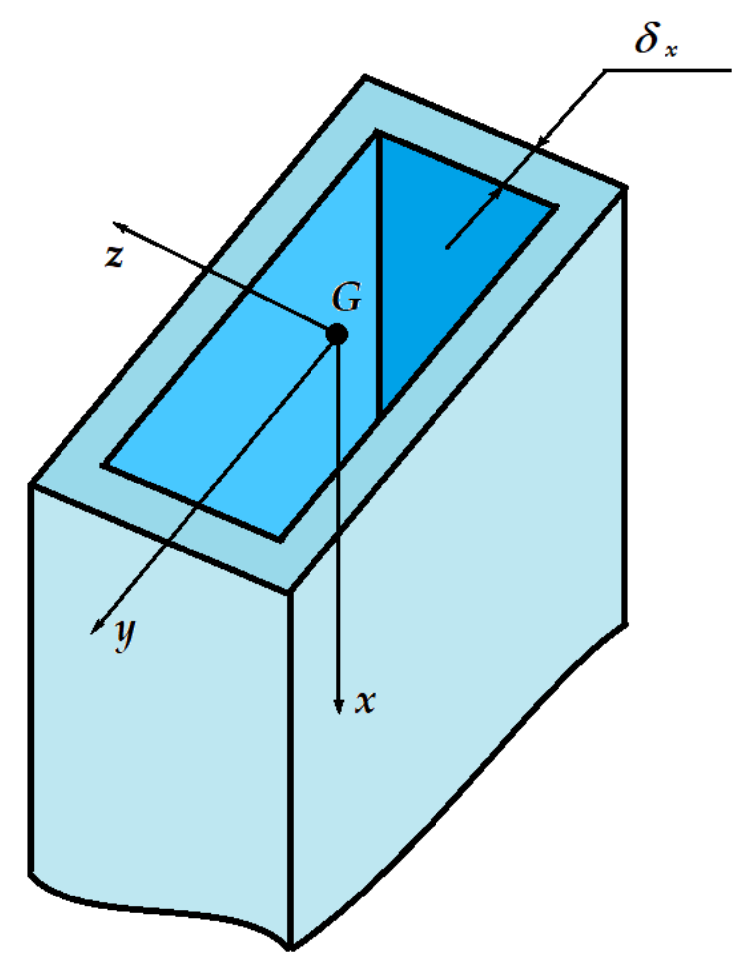
In [29], the authors presented their own research concerning the basic principles of MDA, together with its applicability to heat transfer in bars and bar structures. They deduced, with the help of the MDA briefly described above, the generalized law of the model for a straight bar of tubular–rectangular section, related to the right three-orthogonal reference system (Figure 1).

With these variables, the dimensional sets were established, for two cases considered to be significant, based on the protocol presented in the works of Szirtes [18,19]. Each variable considered to be relevant is defined by the dimensions involved (called the main dimensions) at certain powers. The total number of main dimensions is k. Matrix A, which contains the independent variables, has columns formed by the exponents of these main dimensions related to those variables.

The other variables, i.e., the dependent ones, numbered as n, and which constitute the matrix B, have in the columns afferent to these variables the exponents of the main dimensions, which define the respective variables.

To achieve this, the following were analyzed in detail:

• The variables on which the heat transfer depends in the general case, i.e., the case of a straight bar covered with a layer of intumescent paint;
• Their computational relationships;
• The dimensions of these variables;
• The constituent elements of the dimensional set (DS), specifying the independent variables (those that are freely chosen at the beginning, both for the prototype and for the model) and of the dependent ones (which are freely chosen only for the prototype and for the model results exclusively from the application of the model law, which is deduced).

In [29], the authors presented the basic principles of MDA, together with its applicability to heat transfer in bars and bar structures of circular section. In [30], the authors applied MDA to straight bars of rectangular–tubular section in order to deduce the ML, which governs heat transfer.

Research in the field [31,32,33] proves that in order to obtain similar results, the efforts made with modeling, by application of the model or the experimental measurements to obtain results, require a considerable effort. Other results are presented in [34,35].

This contribution is intended to validate this ML based on a significant number of experimental measurements, performed on a series of prototypes and models, unprotected and thermally protected using layers of intumescent paints. After summarizing the involved variables (see

Table 1. Principal dimensions of the column segment presented in Figure 2.

	Prototype, at Scale 1:1	Model I, at Scale 1:2	Model II, at Scale 1:4
Dimensions, in m
La	0.370	0.185	0.0925
Lb	0.370	0.185	0.0925
Lc	0.006	0.003	0.0015
Ld	0.350	0.175	0.0875
Le	0.350	0.175	0.0875
Lf	0.016	0.008	0.004
Lg	0.016	0.008	0.004
Lh	0.400	0.200	0.100
Lk	0.010	0.005	0.0025
Lm	0.450	0.450	0.450
Ln	0.450	0.450	0.450

) along with the basic elements of the ML, deduced in [30] for two cases relevant from the point of view of experimental measurements, the authors present the set of prototypes and models, based on the case of an actual construction pillar, physically manufactured at scales of 1:1, 1:2, and 1:4. From the combination of these structural elements made at different scales, it resulted in three sets of prototypes and models. New contributions in the domain can be found in [36,37,38,39,40,41,42]. In the next section, the following are presented: the original testing bench of these structural elements; block diagram of the original electronic heating and control system; the basic considerations regarding the particularity of this heating system from the point of view of heat transfer; measurement data, purchased both for nonthermally protected elements and for those protected with layers of intumescent paints. The same thermal regimes were applied to all these structural elements, with registration of all the parameters related to these thermal regimes. Depending on the role of a structural element within a certain set (prototype-model), some of the measurement data were considered as data acquired directly through measurements, and others served as reference elements for those, which we had to obtain through the ML. In the last part of the paper are compared the main sizes of the required dependent variables, obtained by rigorous direct measurements with those offered by the ML on the elements considered as prototypes, respectively, models.

Consequently, these laws can be extended to structural elements, which are achieved at scales of 1:5 and 1:10, respectively, which allow the realization of very convenient models in terms of experimental simulations for complex structures (for example, industrial halls with several compartments and floors having one or more firebreaks arranged as desired). The data of the measurements obtained on these models, i.e., their response to fires, serve by applying these ML to the optimization of actual structures subjected to similar fires.

2. Materials and Methods

Based on results obtained in the abovementioned papers [30,38], two cases were analyzed regarding the choice of the set of independent variables, namely:

• $(Q,L_z,\mathsf{\Delta }t,\tau ,{\lambda }_{x\hspace{0.17em}steel},\varsigma )$;
• $(\dot{Q},L_z,\mathsf{\Delta }t,\tau ,{\lambda }_{x\hspace{0.17em}steel},\varsigma )$,

where $Q$ represents the invested heat; $\dot{Q}$—the heat rate; $L_z$—the beam dimension along direction z; $\mathsf{\Delta }t$—the temperature variation; $\tau$—the time; ${\lambda }_{x\hspace{0.17em}steel}$—the thermal conductivity; and $\varsigma$—the shape factor.

It can be noted that in both cases the set of independent variables is rigorously linked to the actual measurements. Only one dependent variable is an exception, namely that for which we would not have access (or it would be difficult) to obtain its value through measurements. In the latter, the value for the model is chosen in advance (before the start of the experiments) and based on the measurement results, the desired value for the prototype results from the law of the model. In case I it is the heat flow $\dot{Q}$, while in case II it is the amount of heat $Q$.

In order to validate this law, an experimental set consisting of a prototype and two models was designed, starting from the dimensions of an existing structural element (the supporting column of an industrial hall). Thus, for the prototype, made at 1:1 scale, a column segment with height h = 0.400 m was considered; for the two models, it was made at 1:2 and 1:4 scales, having segments with heights h = 0.200 m and h = 0.100 m, respectively (Figure 2 and Table 1).

Table 1 summarizes their dimensions, together with those relating to the seating area on the electric heating stand, shown in Figure 3. As can be seen, the geometric similarity was observed in all of them, accepting the same scales of all dimensions of 1:1, 1:2, and 1:4, respectively.

The upper closing plate, with the dimensions $(L_a x L_b)$, wants to replace the rest of the column, and the lower one, with the dimensions $(L_m x L_n)$, serves to ensure a perfect and unitary placement of all the elements tested on the test stand.

Monitoring of the thermal field propagation along these structural elements was performed with the assistance of thermoresistors, type PT 100–402, with 0.150 m long terminals and measuring range $\left(-70\dots +500 °\mathrm{C}\right)$. Their layout dimensions, starting from the base of the plan (Figure 2), are shown in

Table 2. Principal coordinates of the temperature measuring points.

Prototype, at Scale 1:1	Model I, at Scale 1:2	Model II, at Scale 1:4
Coordinates $x\left(j\right)$
0.020	0.020	0.020
0.110	0.060	0.055
0.200	0.105	0.090
0.290	0.150
0.380	0.190

. At each level were fixed, by means of M3 screws, four thermoresistors (one in the middle of each side), and the average arithmetic of their indications was the temperature of the column segment at that level.

Both the prototype and the two models were subjected to the same heating regimes, in two versions: one that was uncovered and the other covered with a layer of intumescent paint (thermal protection) 0.0012 m thick, type Interchar 404, produced by International Marine and Protective Coatings Co.

According to Figure 3, structural element (1), after a translation, was placed on the upper area of the dome in the form of a pyramid trunk (2), which in turn rests on the rigid frame (3) and on the supporting legs (4).

In section A–A are shown the heating elements (6), consisting of twelve bars/rods of Silite (connected four in series for the three phases of the industrial power supply at 380 V). Silite bars/rods are placed on chamotte bricks (7), under which there is a thermal insulation layer (8) of ceramic fiber 0.0254 m thick. A similar insulation (5) is provided for the lateral side walls of the pyramid trunk (2). During experimental investigations the free surface of the laying board, with dimensions $(L_m x L_n)$, shown in Figure 2, is covered with this thermal insulation blanket. As an illustration of the degree of thermal insulation, it can be mentioned that at the nominal heating temperature of $t_{o,nom}=600 °\mathrm{C}$ of the structural elements tested, around the support frame (3) and the pyramid trunk (2), the temperature did not exceed $(45\hspace{0.17em}\dots 50) °\mathrm{C}$.

Figure 4 shows the set of twelve Silite bars/rods during operation, together with their wiring and thermal insulation. Figure 5, according to [43,44], shows the block diagram of the electronic system for regulating and controlling the temperature at the level of the lower plate of the tested structural element.

Following the analysis of possible solutions, the authors opted for the only acceptable option, namely, to supply heating with whole half-sinusoidal trains having programmable length series, a solution that fully meets the requirements of the experiment with good accuracy [36].

This original electronic system consists in principle of the following basic elements: a digital control circuit (4), which using the synchronization input determines the moment when the main voltage passes through zero. A cycle of ten half-waves (half-sines) is defined, from which, by programming, the required/desired number of half-waves is selected, and by activating the static power relay at the output, this number of half-waves is allowed to pass through the load. These causes the Silite bars/rods to heat while the rest of the half-waves up to ten are blocked. The repetition of ten half-wave cycles is signaled by LED (1). The number of active half-waves is selected using a ten-position selector switch (5); thus, the power introduced in the system is adjusted in steps of 10% from 10% to 90%. For the full power of 100%, switch K1 is actuated, by which the cycles of ten half-periods/half-waves are abandoned, all remaining active. Between the control circuit and the static relay (6), the temperature controller (7) (type ATR121B) is connected, which, through an internal relay contact, validates or stops the heating at the preset power stage. This preset power step is chosen so as to ensure that a temperature slightly higher than that required is reached, and the desired nominal temperature is programmed from the ATR121B temperature controller. The control of the heating elements is performed using static relays (6) of type SSR-4028ZD3 and SSR-4048ZD3, which allow a maximum current of up to 40 (A) and supply voltages of 280 (V) and 480 (V). These static relays, with optical isolation between the control and power terminals, are provided with circuits that ensure to switch on strictly only at the zero crossings of the supply voltage (ZPS—zero point switch), and thus ensure:

• Keeping the sinusoidal shape unaltered, both the supply voltage and the supply current;
• The correct measurement of the electricity consumed/invested in the system, using meters (9), without the appearance of any electromagnetic disturbance in the electrical network.

Measuring the nominal temperature at the base of the tested structural element is made by using a thermocouple, fixed in a suitable bore, which is practiced in the immediate vicinity of junction area. This thermocouple is connected to the ATR121B temperature controller.

The protocol of the experimental investigations was as follows:

• Placing the structural element (1) on the assembled stand by interposing between them, on the effective placement area (effective contact area), a segment of thermal insulating mattress, in order to ensure perfect contact and without thermal losses (Figure 3);
• Mounting on the lower plate of the tested structural element, as close as possible to their junction area, a type-K thermocouple, which is connected to the temperature controller ATR121B, in order to monitor the desired nominal temperature at the base of the structural element;
• Mounting all the type PT 100–402 thermoresistors at the level of the dimensions $x\left(j\right)$ on the tested structural element, according to Table 2;
• Connecting these thermoresistors to the data acquisition system;
• Checking the proper operation of all thermoresistors, and the type-K thermocouple;
• Selection of the nominal temperature $t_{0,\hspace{0.17em}nom}$ on the temperature controller (7) type ATR121B (Figure 5);
• Selecting the desired percentage of supply voltage (Figure 5) on the ten-stage selector switch (5).
• Connection of the heating installation to the 380 V power supply;
• Starting the installation with assistance of the main switch;
• Monitoring, with the help of the data acquisition system, the achievement of the stabilized nominal temperature $t_{0,\hspace{0.17em}nom}$;
• Additional recording, at the thermal level of the stabilized regime, of the consumed electricity $E_{0,\hspace{0.17em}total}\left[\mathrm{k}\mathrm{W}\mathrm{h}\right]$, together with the time necessary ${\tau }_{0,\hspace{0.17em}total}(\mathrm{s})$ to reach this regime;
• Repeating the previous steps, in order to reach all the nominal temperatures $t_{0,\hspace{0.17em}nom}=(100, 200, 300, 400, 450, 500) °\mathrm{C}$.

Observations:

• The ATR121B temperature controller also has a self-learning function, practically, after the first cycle of reaching the nominal temperature $t_{0,\hspace{0.17em}nom}$, it will ensure the temperature regulation within very limited range. Thus, for example, based on the measurements performed at one $t_{0,\hspace{0.17em}nom}=500 °\mathrm{C}$, the thermal oscillations related to the adjustment were of maximum $(4\dots 5) °\mathrm{C}$;
• Attaining a stabilized temperature regime was considered to be achieved when the level of the last thermoresistance PT 100–402 (near the upper part of the tested structural element) maximum temperature oscillations $(0.2\dots 0.3) °\mathrm{C}$ were observed for a minimum period of $\left(120\dots 180\right) \mathrm{s}$.

3. Results

After reaching this stabilized regime, the total amount of electricity invested in the system from the beginning of the heating process $E_{0,\hspace{0.17em}total}\left[\mathrm{k}\mathrm{W}\mathrm{h}\right]$ was read, which corresponded, in the hypothesis of a transformation without energy losses, a total amount of heat invested in the stand:

$$Q_{0,\hspace{0.17em}total}\left[\mathrm{J}\right]=E_{0,\hspace{0.17em}total}\left[\mathrm{k}\mathrm{W}\mathrm{h}\right]\cdot 3.6\cdot {10}^6,$$

(1)

since $1\hspace{0.17em}\mathrm{k}\mathrm{W}\mathrm{h}=3600\hspace{0.17em}\mathrm{k}\mathrm{W}\mathrm{s}=3600\hspace{0.17em}\mathrm{k}\mathrm{J}=3.6\cdot {10}^6 \mathrm{J}$.

The total heat losses through the thermal insulation blankets are determined based on the well-known relationship

$$Q_{waste,\hspace{0.17em}total}=Q_{w,\hspace{0.17em}total}={\displaystyle \sum [\lambda \cdot \mathsf{\Delta }t\cdot \mathsf{\Delta }\tau }\cdot ({\displaystyle \sum \frac{A_k}{h_k}})],$$

(2)

where $\lambda \left[\frac{W}{m\cdot K}=\frac{W}{m\cdot °\mathrm{C}}\right]$ is the coefficient of thermal conductivity of the thermal insulation blanket, which, based on the recommendation of the manufacturing company for the material used, depending on the temperature reached $t\left[°\mathrm{C}\right]$ at the level of its heated side, has the calculation relationship

$$\lambda \left[\frac{W}{m\cdot °\mathrm{C}}\right]=0.0002\cdot t\left[°\mathrm{C}\right]+0.03,$$

(3)

• $\mathsf{\Delta }t\left[°\mathrm{C}\right]$—the temperature difference reached during heating;
• $\mathsf{\Delta }\tau \left[\mathrm{s}\right]$—the time required to reach it;
• $A_k\left[{\mathrm{m}}^2\right]$—the developed/unfolded areas of the all $k$ thermal insulation layers applied around the stand, having the thicknesses $h_k\left[m\right]$.

However, we must also take into account the particularity of the heating system through the thermoregulation presented above, because instead of a linear law of temperature increasing from $t_B\equiv t_i$ to $t_D\equiv t_n$ (shown with the dashed line in Figure 6), the actual data acquisition resulted in a polygon $(B\equiv i\hspace{0.17em}-\hspace{0.17em}j\hspace{0.17em}-\hspace{0.17em}k\hspace{0.17em}-\hspace{0.17em}l\hspace{0.17em}-\hspace{0.17em}m\hspace{0.17em}-\hspace{0.17em}n\equiv D)$, to which relations (2) and (3) must be adapted, as follows:

• In relation (2), for each interval $(i-j);(j-k);(k-l);(l-m);(m-n)$ is considered the corresponding temperature difference ($\mathsf{\Delta }{t}_{ij}=\left(t_j-t_i\right)$; $\mathsf{\Delta }{t}_{jk}=\left(t_k-t_j\right)$; $\mathsf{\Delta }{t}_{kl}=\left(t_l-t_k\right)$; $\mathsf{\Delta }{t}_{lm}=\left(t_m-t_l\right)$; $\mathsf{\Delta }{t}_{mn}=\left(t_n-t_m\right)$), applied to the corresponding time intervals $\mathsf{\Delta }\tau$: $\mathsf{\Delta }{\tau }_{ij}=\left({\tau }_j-{\tau }_i\right)$; $\mathsf{\Delta }{\tau }_{jk}=\left({\tau }_k-{\tau }_j\right)$; $\mathsf{\Delta }{\tau }_{kl}=\left({\tau }_l-{\tau }_k\right)$; $\mathsf{\Delta }{\tau }_{lm}=\left({\tau }_m-{\tau }_l\right)$; $\mathsf{\Delta }{\tau }_{mn}=\left({\tau }_n-{\tau }_m\right)$;
• $\lambda$ is determined with the relation (3) separately/individually for each previous interval, considering the average temperature afferent to each interval, respectively, the previous temperature differences;
• The term ${\displaystyle \sum \frac{A_k}{h_k}}$ being constant, multiplies the sum of the partial products $\left(\lambda \cdot \mathsf{\Delta }t\cdot \mathsf{\Delta }\tau \right)$ related to these intervals.

The total amount of heat invested for heating the structural element $Q_{total}\left[\mathrm{J}\right]$ is obtained as the difference of the previous ones, i.e.,

$$Q_{total}\left[\mathrm{J}\right]=Q_{0,\hspace{0.17em}total}-Q_{w,\hspace{0.17em}total}.$$

(4)

The thermal radiation of the Silite bars/rods manifests itself only in an experimentally determined proportion of 47.22% on the lower support plate of the structural element, corresponding to the angle of $\frac{42.77}{100}\ast 360=169.992\cong 2\cdot {85}^{°}$ from the total ${360}^{°}$ (Figure 7), then the amount of actual heat invested in the system can be defined, i.e.,

$$Q_{eff}\left[\mathrm{J}\right]=Q_{0,eff}-Q_{w,\hspace{0.17em}total}=0.4722\cdot Q_{0,\hspace{0.17em}total}-Q_{w,\hspace{0.17em}total}.$$

(5)

Obviously, there is a global approximation of the direct heating provided by the Silite bars. It should be mentioned that the ML has been verified (and validated accordingly) for this last customization as well.

The corresponding heat fluxes are determined on the basis of the definition relation:

$$\dot{Q}\left[\frac{J}{s}=W\right]=\frac{dQ}{d\tau }=\frac{\mathsf{\Delta }Q}{\mathsf{\Delta }\tau },$$

(6)

It is obvious that the quantities of heat, the heat flows, and the times necessary to reach higher thermal regimes were determined by summing the last values with those previously obtained.

Thus, for example, the parameters related to reaching the stabilized regime at $t_{0,\hspace{0.17em}nom}=200 °\mathrm{C}$ resulted from the sum of the values obtained for the stabilized regime from $t_{0,\hspace{0.17em}nom}=100 °\mathrm{C}$ with those obtained during the heating of the system in the temperature range $\left(100\dots 200\right) °\mathrm{C}$.

Table 3. Small model, unpainted—scale 1:4; values of the dependent variables by the ML.

1	$\mathsf{\Delta }t\hspace{0.17em}(°\mathrm{C})$	23–100	100–200	200–300	300–400	400–450	450–500
2	$\varsigma \left(\frac{1}{m_y}\right)$	261,976	261,976	261,976	261,976	261,976	261,976
3	$E_{0,\hspace{0.17em}total}\left(\mathrm{k}\mathrm{W}\mathrm{h}\right)$	0.4	0.6	1.4	1.4	2.9	0.7
4	$Q_{0,\hspace{0.17em}total}\left(\mathrm{J}\right)$	1,440,000	2,160,000	5,040,000	5,040,000	10,440,000	2,520,000
5	$\mathsf{\Delta }{t}_{total}\left(°\mathrm{C}\right)$	77	100	100	100	50	50
6	${\displaystyle \sum \frac{A_k}{h_k}}\left(\mathrm{m}\right)$	20.07	20.07	20.07	20.07	20.07	20.07
7	$Q_{w,total}\left(\mathrm{J}\right)$	84,810.39	185,272.30	1,000,576	1,018,576	2,709,526	572,461.50
8	$Q_{total}\left(\mathrm{J}\right)$	1,355,190	1,974,728	4,039,424	4,021,424	7,730,474	1,947,539
9	$Q_{o,\hspace{0.17em}eff}\left(\mathrm{J}\right)$	679,968	1,019,952	2,379,888	2,379,888	4,929,768	1,189,944
10	$Q_{eff}\left(\mathrm{J}\right)$	595,158	834,680	1,379,312	1,361,312	2,220,242	617,483
11	$\mathsf{\Delta }{\tau }_{total}\left(\mathrm{s}\right)$	2280	1320	3000	1800	3600	660
12	${\dot{Q}}_{w,\hspace{0.17em}total}\left(\mathrm{J}\right)$	37.20	140.36	333.53	565.88	752.65	867.37
13	${\dot{Q}}_{total}\left(\mathrm{W}\right)$	594.38	1496.01	1346.48	2234.13	2147.35	2950.82
14	${\dot{Q}}_{eff}\left(\mathrm{W}\right)$	261.03	632.33	459.77	756.28	616.73	935.58

,

Table 4. Small model, painted—scale 1:4; values of the dependent variables by the ML.

1	$\mathsf{\Delta }t\hspace{0.17em}(°\mathrm{C})$	23–100	100–200	200–300	300–400	400–450	450–500
2	$\varsigma \left(\frac{1}{m_y}\right)$	261,976	261,976	261,976	261,976	261,976	261,976
3	$E_{0,\hspace{0.17em}total}\left(\mathrm{k}\mathrm{W}\mathrm{h}\right)$	0.4	1.0	1.6	1.0	0.9	2.3
4	$Q_{0,\hspace{0.17em}total}\left(\mathrm{J}\right)$	1,440,000	3,600,000	5,760,000	3,600,000	3,240,000	8,280,000
5	$\mathsf{\Delta }{t}_{total}\left(°\mathrm{C}\right)$	77	100	100	100	50	50
6	${\displaystyle \sum \frac{A_k}{h_k}}\left(\mathrm{m}\right)$	20.07	20.07	20.07	20.07	20.07	20.07
7	$Q_{w,total}\left(\mathrm{J}\right)$	73,312	411,563	1,016,682	685,260	706,478	2,287,113
8	$Q_{total}\left(\mathrm{J}\right)$	1,366,688	3,188,436	4,743,318	2,914,740	2,533,521	5,992,887
9	$Q_{o,\hspace{0.17em}eff}\left(\mathrm{J}\right)$	679,968	1,699,920	2,719,872	1,699,920	1,529,928	3,909,816
10	$Q_{eff}\left(\mathrm{J}\right)$	606,655	1,288,356	1,703,190	1,014,660	823,449	1,622,703
11	$\mathsf{\Delta }{\tau }_{total}\left(\mathrm{s}\right)$	2220	3720	3180	1320	1020	2700
12	${\dot{Q}}_{w,\hspace{0.17em}total}\left(\mathrm{J}\right)$	33.02	110.64	319.71	519.14	692.63	847.08
13	${\dot{Q}}_{total}\left(\mathrm{W}\right)$	615.63	857.11	1491.61	2208.14	2483.84	2219.59
14	${\dot{Q}}_{eff}\left(\mathrm{W}\right)$	273.27	346.33	535.59	768.68	807.30	601.00

,

Table A2. Middle model, unpainted—scale 1:2.

1	$\mathsf{\Delta }t\hspace{0.17em}(°\mathrm{C})$	23–100	100–200	200–300	300–400	400–450	450–500
2	$\varsigma \left(\frac{1}{m_y}\right)$	130,988	130,988	130,988	130,988	130,988	130,988
3	$E_{0,\hspace{0.17em}total}\left(\mathrm{k}\mathrm{W}\mathrm{h}\right)$	0.6	1.1	0.8	1.3	0.8	1.2
4	$Q_{0,\hspace{0.17em}total}\left(\mathrm{J}\right)$	2,160,000	3,960,000	2,880,000	4,680,000	2,880,000	4,320,000
5	$\mathsf{\Delta }{t}_{total}\left(°\mathrm{C}\right)$	77	100	100	100	50	50
6	${\displaystyle \sum \frac{A_k}{h_k}}\left(\mathrm{m}\right)$	19.17	19.17	19.17	19.17	19.17	19.17
7	$Q_{w,\hspace{0.17em}total}\left(\mathrm{J}\right)$	32,233	324,889	244,466	619,849	389.373	667,908
8	$Q_{total}\left(\mathrm{J}\right)$	2,127,767	3,635,110	2,635,533	4,060,150	2,490,627	3,652,091
9	$Q_{o,\hspace{0.17em}eff}\left(\mathrm{J}\right)$	1,019,952	1,869,912	1,359,936	2,209,896	1,359,936	2,039,904
10	$Q_{eff}\left(\mathrm{J}\right)$	987,719	1,545,022	1,115,469	1,590,046	970,563	1,371,995
11	$\mathsf{\Delta }{\tau }_{total}\left(\mathrm{s}\right)$	1260	2400	900	1260	600	840
12	${\dot{Q}}_{w,\hspace{0.17em}total}\left(\mathrm{J}\right)$	25.58	135.37	271.62	491.94	648.96	795.13
13	${\dot{Q}}_{total}\left(\mathrm{W}\right)$	1688.70	1514.63	2928.37	3222.34	4151.05	4347.73
14	${\dot{Q}}_{eff}\left(\mathrm{W}\right)$	783.90	643.76	1239.41	1261.94	1617.61	1633.33

,

Table A3. Prototype, unpainted—scale 1:1.

1	$\mathsf{\Delta }t\hspace{0.17em}(°\mathrm{C})$	23–100	100–200	200–300	300–400	400–450	450–500
2	$\varsigma \left(\frac{1}{m_y}\right)$	65.49	65.49	65.49	65.49	65.49	65.49
3	$E_{0,\hspace{0.17em}total}\left(\mathrm{k}\mathrm{W}\mathrm{h}\right)$	0.9	1.4	2.3	2.8	1.6	2.7
4	$Q_{0,\hspace{0.17em}total}\left(\mathrm{J}\right)$	3,240,000	5,040,000	8,280,000	10,080,000	5,760,000	9,720,000
5	$\mathsf{\Delta }{t}_{total}\left(°\mathrm{C}\right)$	77	100	100	100	50	50
6	${\displaystyle \sum \frac{A_k}{h_k}}\left(\mathrm{m}\right)$	15.55	15.55	15.55	15.55	15.55	15.55
7	$Q_{w,\hspace{0.17em}total}\left(\mathrm{J}\right)$	41,696	323,210	391,377	510,624	459,366	777,565
8	$Q_{total}\left(\mathrm{J}\right)$	3,198,303	4,716,790	7,888,623	9,569,375	5,300,633	8,942,435
9	$Q_{o,\hspace{0.17em}eff}\left(\mathrm{J}\right)$	1,529,928	2,379,888	3,909,816	4,759,776	2,719,872	4,589,784
10	$Q_{eff}\left(\mathrm{J}\right)$	1,488,231	2,056,678	3,518,439	4,249,151	2,260,505	3,812,219
11	$\mathsf{\Delta }{\tau }_{total}\left(\mathrm{s}\right)$	1860	2880	1560	1200	780	1080
12	${\dot{Q}}_{w,\hspace{0.17em}total}\left(\mathrm{J}\right)$	22.42	112.23	250.88	425.52	588.93	719.97
13	${\dot{Q}}_{total}\left(\mathrm{W}\right)$	1719.52	1637.77	5056.81	7974.48	6795.68	8280.03
14	${\dot{Q}}_{eff}\left(\mathrm{W}\right)$	800.12	714.12	2255.41	3.540.96	2898.08	3529.83

,

Table A4. Middle model painted—scale 1:2.

1	$\mathsf{\Delta }t\hspace{0.17em}(°\mathrm{C})$	23–100	100–200	200–300	300–400	400–450	450–500
2	$\varsigma \left(\frac{1}{m_y}\right)$	130,988	130,988	130,988	130,988	130,988	130,988
3	$E_{0,\hspace{0.17em}total}\left(\mathrm{k}\mathrm{W}\mathrm{h}\right)$	0.6	1.3	1.0	1.6	0.7	0.8
4	$Q_{0,\hspace{0.17em}total}\left(\mathrm{J}\right)$	2,160,000	4,680,000	3,600,000	5,760,000	2,520,000	2,880,000
5	$\mathsf{\Delta }{t}_{total}\left(°\mathrm{C}\right)$	77	100	100	100	50	50
6	${\displaystyle \sum \frac{A_k}{h_k}}\left(\mathrm{m}\right)$	19.17	19.17	19.17	19.17	19.17	19.17
7	$Q_{w,total}\left(\mathrm{J}\right)$	35,855	329,676	277,713	823,809	368,480	544,542
8	$Q_{total}\left(\mathrm{J}\right)$	2,124,145	4,350,324	3,322,287	4,936,191	2,151,519	2,335,458
9	$Q_{o,\hspace{0.17em}eff}\left(\mathrm{J}\right)$	1,019,952	2,209,896	1,699,920	2,719,872	1,189,944	1,359,936
10	$Q_{eff}\left(\mathrm{J}\right)$	984,097	1,880,220	1,422,207	1,896,063	821,463	815,394
11	$\mathsf{\Delta }{\tau }_{total}\left(\mathrm{s}\right)$	1260	2520	960	1560	540	660
12	${\dot{Q}}_{w,\hspace{0.17em}total}\left(\mathrm{J}\right)$	28.46	130.82	289.28	528.08	682.37	825.06
13	${\dot{Q}}_{total}\left(\mathrm{W}\right)$	1685.83	1726.32	3460.72	3164.23	3984.30	3538.57
14	${\dot{Q}}_{eff}\left(\mathrm{W}\right)$	781.03	746.12	1481.47	1215.43	1521.23	1235.45

and

Table A5. Prototype painted—scale 1:1.

1	$\mathsf{\Delta }t\hspace{0.17em}(°\mathrm{C})$	23–100	100–200	200–300	300–400	400–450	450–500
2	$\varsigma \left(\frac{1}{m_y}\right)$	65,494	65,494	65,494	65,494	65,494	65,494
3	$E_{0,\hspace{0.17em}total}\left(\mathrm{k}\mathrm{W}\mathrm{h}\right)$	1.3	2.9	2.2	2.0	1.2	1.4
4	$Q_{0,\hspace{0.17em}total}\left(\mathrm{J}\right)$	4,680,000	10,440,000	7,920,000	7,200,000	4,320,000	5,040,000
5	$\mathsf{\Delta }{t}_{total}\left(°\mathrm{C}\right)$	77	100	100	100	50	50
6	${\displaystyle \sum \frac{A_k}{h_k}}\left(\mathrm{m}\right)$	15.55	15.55	15.55	15.55	15.55	15.55
7	$Q_{w,total}\left(\mathrm{J}\right)$	34,080	426,291	343,503	330,213	242,363	515,675
8	$Q_{total}\left(\mathrm{J}\right)$	4,645,920	10,013,709	7,576,497	6,869,786	4,077,637	4,524,325
9	$Q_{o,\hspace{0.17em}eff}\left(\mathrm{J}\right)$	2,209,896	4,929,768	3,739,824	3,399,840	2,039,904	2,379,888
10	$Q_{eff}\left(\mathrm{J}\right)$	2,175,816	4,503,477	3,396,321	3,069,627	1,797,541	1,864,213
11	$\mathsf{\Delta }{\tau }_{total}\left(\mathrm{s}\right)$	1680	3960	1560	900	480	840
12	${\dot{Q}}_{w,\hspace{0.17em}total}\left(\mathrm{J}\right)$	20.29	107.65	220.19	366.90	504.92	613.90
13	${\dot{Q}}_{total}\left(\mathrm{W}\right)$	2765.43	2528.72	4856.73	7633.010	8495.08	5386.10
14	${\dot{Q}}_{eff}\left(\mathrm{W}\right)$	1295.13	1137.24	2177.13	3410.70	3744.88	2219.30

summarize these preliminary calculations, based on data acquired from all structural elements subjected to the tests (prototype and the two models) uncovered and, respectively, covered with a layer of intumescent paint.

In order to validate the ML in the two versions (I and II), all the calculations related to the significant variables involved were performed.

In the case of version I, where the set of independent variables was $(Q, L_z, \mathsf{\Delta }t, \tau , \hspace{0.17em}{\lambda }_{x\hspace{0.17em}steel}, \varsigma )$, the main dependent variable remained the heat flow $\dot{Q}$, which had to be determined with the help of the ML for the prototype (based on the measurements performed on the model).

Similarly, in the case of version II, where the set of independent variables was $(\dot{Q}, L_z, \mathsf{\Delta }t, \tau , {\lambda }_{x\hspace{0.17em}steel}, \varsigma )$, the dependent variable sought for the prototype became the amount of heat $Q$.

Obviously, in these experimental investigations, all the variables mentioned above were known (being determined by effective measurements), but the problem was to find the values of the dependent variables by the ML, depending on the chosen version (versions I and II), just to validate the model law (Table 3 and Table 4). The other case is presented in the Appendix A and Appendix B (

Table A1. Nomenclature and symbols in DA.

Name of Variable	Symbol/Formula
Area (m2)	A
Constant-pressure specific heat (J/°C)	$c_p=\frac{1}{m}\cdot \frac{dQ}{dt}$
Specific heat capacity (J/°C)	$C=\frac{dQ}{dT}$
Force (N)	F
Gravitational acceleration (m/s2)	g
Length (m)	l, L
Cross-section perimeter (m)	P
Heat $\left(\mathrm{J}\right) {}^{(*)}$	Q
Heat rate (W)	$\dot{Q}=\frac{dQ}{d\tau }$
Temperature (°C)	t, T
Velocity $(\mathrm{m}/\mathrm{s}) {}^{(**)}$	wo
Developed areas (m2)	Ak
Scale factor corresponding to the sizes indicated in the index.	$S_{\dot{Q}}\hspace{0.17em},\hspace{0.17em}\hspace{0.17em}{S}_{L_z}\hspace{0.17em},\hspace{0.17em}\hspace{0.17em}{S}_{\mathsf{\Delta }t}\hspace{0.17em},\hspace{0.17em}{S}_{\tau }\hspace{0.17em},\hspace{0.17em}\hspace{0.17em}{S}_{{\lambda }_{x\hspace{0.17em}steel}}\hspace{0.17em},S_{\varsigma }$
Coefficient of volume expansion °C	$\beta$
Variation	$\mathsf{\Delta }$
Thermal conductivity (W/(m °C))	$\lambda$
Time, shear stress (s, N/m2)	$\tau$
Density (steel, air, paint/insulating material) (kg/m3)	$\rho$
Thermal conductivity (steel, paint coat), along directions	${\lambda }_x; {\lambda }_y\hspace{0.17em}; {\lambda }_z$
Thermal diffusivity of air, along directions (m2/s)	$a_x=\frac{{\lambda }_x}{\rho \cdot c_p}$$;a_y=\frac{{\lambda }_y}{\rho \cdot c_p}$$;a_z=\frac{{\lambda }_z}{\rho \cdot c_p}$
Dynamic viscosity of air, along directions (kg/ms)	${\eta }_x=\frac{{\tau }_{0,x}}{\nabla w_0}=\frac{F_{0,x}}{A_{xy}}\cdot \frac{1}{\nabla w_0}$$;{\eta }_y=\frac{{\tau }_{0,y}}{\nabla w_0}=\frac{F_{0,y}}{A_{zy}}\cdot \frac{1}{\nabla w_0}$; ${\eta }_z=\frac{{\tau }_{0,z}}{\nabla w_0}=\frac{F_{0,z}}{A_{yz}}\cdot \frac{1}{\nabla w_0}$
Kinematic viscosity of air, along directions (m2/s)	${\nu }_x=\frac{{\eta }_x}{\rho }=\frac{1}{\rho }\cdot {\eta }_x\hspace{0.17em}$$;{\nu }_y=\frac{{\eta }_y}{\rho }=\frac{1}{\rho }\cdot {\eta }_y\hspace{0.17em}\hspace{0.17em}$$;{\nu }_z=\frac{{\eta }_z}{\rho }=\frac{1}{\rho }\cdot {\eta }_z\hspace{0.17em}$
Prandtl number of air, along directions	${Pr}_x={\nu }_x\cdot \frac{1}{a_x}$$;{Pr}_y={\nu }_y\cdot \frac{1}{a_y}$$;{Pr}_z={\nu }_z\cdot \frac{1}{a_z}$
Reynolds number, along directions	${Re}_x=\frac{w_{0,\hspace{0.17em}x}\cdot l_x}{{\nu }_x}$$;{Re}_y=\frac{w_{0,\hspace{0.17em}y}\cdot l_y}{{\nu }_y}$$;{Re}_z=\frac{w_{0,\hspace{0.17em}z}\cdot l_z}{{\nu }_z}$
Convection heat transfer coefficient, along directions ${}^{(***)}$ (W/(m2 °C));	${\alpha }_{nx}$$; {\alpha }_{ny}$$; {\alpha }_{nz}$
Thickness of the paint coat, along directions (m)	$d_y={\delta }_y$$; d_z={\delta }_z$
Volume of bar or paint coat (m3)	$V$
Area of the bar cross-section	$A_{tr}$
Lateral area (x-z)	${A^{\prime }}_{lat}$
Lateral area (x-y)	${A^{″}}_{lat}$
Bar dimensions	$L_x$$; L_y$$; L_z$
Shape factor (m−1)	$\varsigma =\frac{A_{lat}}{V}=\frac{P}{A_{tr}}$
Temperature variation	$\mathsf{\Delta }T/\mathsf{\Delta }t$
Nusselt number, along directions	$N{u}_x=\frac{{\alpha }_x\cdot l_x}{{\lambda }_{f,\hspace{0.17em}\hspace{0.17em}x}}$$;N{u}_y=\frac{{\alpha }_y\cdot l_y}{{\lambda }_{f,\hspace{0.17em}\hspace{0.17em}y}}$$;N{u}_z=\frac{{\alpha }_z\cdot l_z}{{\lambda }_{f,\hspace{0.17em}z}}$
Grashof number, along directions	$G{r}_x=\frac{g\cdot \beta \cdot \mathsf{\Delta }t\cdot l_{\zeta }^3}{{\nu }_{\zeta }^2}$
Péclet number, along directions	$P{e}_x={\mathrm{Re}}_x\cdot {\mathrm{Pr}}_x$$;P{e}_y={\mathrm{Re}}_y\cdot {\mathrm{Pr}}_y$$;P{e}_z={\mathrm{Re}}_z\cdot {\mathrm{Pr}}_z$
Biot number, along directions	$B{i}_x=\frac{{\alpha }_x\cdot l_x}{{\lambda }_{s,\hspace{0.17em}x}}$$;B{i}_y=\frac{{\alpha }_y\cdot l_y}{{\lambda }_{s,\hspace{0.17em}y}}$$;B{i}_z=\frac{{\alpha }_z\cdot l_z}{{\lambda }_{s,\hspace{0.17em}z}}$
Stanton number, along directions	$S{t}_x=\frac{N{u}_x}{P{e}_x}$$;S{t}_y=\frac{N{u}_y}{P{e}_y}$$;S{t}_y=\frac{N{u}_y}{P{e}_y}$
Fourier number, along directions	$F{o}_x=\frac{a_x\cdot \mathsf{\Delta }\tau }{l_x^2}$$;F{o}_y=\frac{a_y\cdot \mathsf{\Delta }\tau }{l_y^2}$$;F{o}_z=\frac{a_z\cdot \mathsf{\Delta }\tau }{l_z^2}$

${}^{(*)}$ It is considered to be numerically equal to the dimension of work; the work is conventionally considered as a product between a force having the direction along the bar, $F_x\hspace{0.17em}(N_x=\frac{kg.m_x}{s^2})$ and the displacement along the same direction x ($m_x$). ${}^{(**)}$ The velocity $w_0$ is normal to the plane where the shear stress is developed; $\nabla w_0$ represents its gradient. ${}^{(***)}$ When the bar is protected (insulated) by a paint coat, then ${{\alpha }^{\prime }}_{nf}={\alpha }_{ny}$ and ${{\alpha }^{″}}_{nf}={\alpha }_{nz}$.

, Table A2, Table A3, Table A4 and Table A5).

In order to perform a very rigorous analysis, the following prototype-model sets were considered, both for the unprotected versions and for those protected with intumescent paint. The pairs of versions are:

• Prototype (structural element made at 1:1 scale) + Model (structural element made at 1:2 scale), symbolized by (1: 2/1:1) Model/Prototype;
• Prototype (structural element made at 1:2 scale) + Model (structural element made at 1:4 scale), symbolized by (1:4/1:2) Model/Prototype;
• Prototype (structural element made at 1:1 scale) + Model (structural element made at 1:4 scale), symbolized by (1:4/1:1) Model/Prototype.

Taking into account the simplifications analyzed in the previous observations, in

Table 5. The 1:2/1:1 unpainted model/prototype; measured values.

1	Measured	$\mathsf{\Delta }t\hspace{0.17em}\left(°\mathrm{C}\right)$	$\mathsf{\Delta }t\hspace{0.17em}\left[°\mathrm{C}\right]$	23–100	100–200	200–300	300–400	400–450	450–500
2		$S_{\varsigma }\left(-\right)$	$S_{\varsigma }\hspace{0.17em}\left[-\right]$	2	2	2	2	2	2
3		$S_{\mathsf{\Delta }{\tau }_{total}}\hspace{0.17em}\left(-\right)$	$S_{\mathsf{\Delta }{\tau }_{total}}\hspace{0.17em}\left[-\right]$	0.6774	0.8333	0.5769	1.05	0.7692	0.7777
4		$S_{{\dot{Q}}_{total}}\left(-\right)$	$S_{Q_{total}}\left[-\right]$	0.665	0.771	0.334	0.424	0.470	0.408
5		$S_{{\dot{Q}}_{eff}}\left(-\right)$	$S_{Q_{eff}}\left[-\right]$	0.664	0.751	0.317	0.374	0.429	0.360
6	Verification	$S_{A_{tr}}\hspace{0.17em}\left(-\right)$	$S_{A_{tr}}\hspace{0.17em}\left[-\right]$	0.25	0.25	0.25	0.25	0.25	0.25
7		$S_{L_y\hspace{0.17em}}\left(-\right)$	$S_{L_y\hspace{0.17em}}\left[-\right]$	0.5	0.5	0.5	0.5	0.5	0.5
8		$S_{Q_{total}}\left(-\right)$	$S_{{\dot{Q}}_{total}}\left[-\right]$	0.928	0.925	0.579	0.404	0.611	0.525
9		$S_{Q_{eff}}\left(-\right)$	$S_{{\dot{Q}}_{eff}}\left[-\right]$	0.980	0.901	0.550	0.356	0.558	0.463
10	Calculated with the Model Law	$S_{Q_{total}}\left(-\right)$	$S_{{\dot{Q}}_{total}}\left[-\right]$	0.982	0.925	0.579	0.404	0.611	0.525
11		$S_{Q_{eff}}\left(-\right)$	$S_{{\dot{Q}}_{eff}}\left[-\right]$	0.980	0.901	0.550	0.356	0.558	0.463
12		$S_{A_{tr}}\hspace{0.17em}\left(-\right)$	$S_{A_{tr}}\hspace{0.17em}\left[-\right]$	0.25	0.25	0.25	0.25	0.25	0.25
13		$S_{L_y\hspace{0.17em}}\left(-\right)$	$S_{L_y\hspace{0.17em}}\left[-\right]$	0.5	0.5	0.5	0.5	0.5	0.5

and

Table 6. The 1:2/1:1 Painted model/prototype; measured values.

1	Measured	$\mathsf{\Delta }t\hspace{0.17em}\left(°\mathrm{C}\right)$	$\mathsf{\Delta }t\hspace{0.17em}\left[°\mathrm{C}\right]$	23–100	100–200	200–300	300–400	400–450	450–500
2		$S_{\varsigma }\left(-\right)$	$S_{\varsigma }\hspace{0.17em}\left[-\right]$	2	2	2	2	2	2
3		$S_{\mathsf{\Delta }{\tau }_{total}}\hspace{0.17em}\left(-\right)$	$S_{\mathsf{\Delta }{\tau }_{total}}\hspace{0.17em}\left[-\right]$	0.750	0.636	0.615	1.733	1.125	0.786
4		$S_{{\dot{Q}}_{total}}\left(-\right)$	$S_{Q_{total}}\left[-\right]$	0.457	0.434	0.438	0.719	0.528	1.027
5		$S_{{\dot{Q}}_{eff}}\left(-\right)$	$S_{Q_{eff}}\left[-\right]$	0.452	0.418	0.419	0.618	0.457	0.437
6	Verification	$S_{A_{tr}}\hspace{0.17em}\left(-\right)$	$S_{A_{tr}}\hspace{0.17em}\left[-\right]$	0.25	0.25	0.25	0.25	0.25	0.25
7		$S_{L_y\hspace{0.17em}}\left(-\right)$	$S_{L_y\hspace{0.17em}}\left[-\right]$	0.5	0.5	0.5	0.5	0.5	0.5
8		$S_{Q_{total}}\left(-\right)$	$S_{{\dot{Q}}_{total}}\left[-\right]$	0.609	0.683	0.713	0.415	0.469	0.657
9		$S_{Q_{eff}}\left(-\right)$	$S_{{\dot{Q}}_{eff}}\left[-\right]$	0.603	0.656	0.680	0.356	0.406	0.557
10	Calculated with the Model Law	$S_{Q_{total}}\left(-\right)$	$S_{{\dot{Q}}_{total}}\left[-\right]$	0.609	0.683	0.713	0.415	0.469	0.657
11		$S_{Q_{eff}}\left(-\right)$	$S_{{\dot{Q}}_{eff}}\left[-\right]$	0.603	0.656	0.680	0.356	0.406	0.557
12		$S_{A_{tr}}\hspace{0.17em}\left(-\right)$	$S_{A_{tr}}\hspace{0.17em}\left[-\right]$	0.25	0.25	0.25	0.25	0.25	0.25
13		$S_{L_y\hspace{0.17em}}\left(-\right)$	$S_{L_y\hspace{0.17em}}\left[-\right]$	0.5	0.5	0.5	0.5	0.5	0.5

are summarized the results of these calculations for version I, and in

Table 7. The 1:2/1:1 unpainted model/prototype; measured values.

1	Measured	$\mathsf{\Delta }t\hspace{0.17em}\left(°\mathrm{C}\right)$	$\mathsf{\Delta }t\hspace{0.17em}\left[°\mathrm{C}\right]$	23–100	100–200	200–300	300–400	400–450	450–500
2		$S_{\varsigma }\left(-\right)$	$S_{\varsigma }\hspace{0.17em}\left[-\right]$	2	2	2	2	2	2
3		$S_{\mathsf{\Delta }{\tau }_{total}}\hspace{0.17em}\left(-\right)$	$S_{\mathsf{\Delta }{\tau }_{total}}\hspace{0.17em}\left[-\right]$	0.677	0.833	0.577	1.05	0.769	0.778
4		$S_{{\dot{Q}}_{total}}\left(-\right)$	$S_{{\dot{Q}}_{total}}\left[-\right]$	0.982	0.925	0.579	0.404	0.611	0.525
5		$S_{{\dot{Q}}_{eff}}\left(-\right)$	$S_{{\dot{Q}}_{eff}}\left[-\right]$	0.980	0.901	0.549	0.356	0.558	0.463
6	Verification	$S_{A_{tr}}\hspace{0.17em}\left(-\right)$	$S_{A_{tr}}\hspace{0.17em}\left[-\right]$	0.25	0.25	0.25	0.25	0.25	0.25
7		$S_{L_y\hspace{0.17em}}\left(-\right)$	$S_{L_y\hspace{0.17em}}\left[-\right]$	0.5	0.5	0.5	0.5	0.5	0.5
8		$S_{Q_{total}}\left(-\right)$	$S_{Q_{total}}\left[-\right]$	0.665	0.771	0.334	0.424	0.470	0.408
9		$S_{Q_{eff}}\left(-\right)$	$S_{Q_{eff}}\left[-\right]$	0.664	0.751	0.317	0.374	0.429	0.359
10	Calculated with the Model Law	$S_{Q_{total}}\left(-\right)$	$S_{Q_{total}}\left[-\right]$	0.665	0.771	0.334	0.424	0.470	0.408
11		$S_{Q_{eff}}\left(-\right)$	$S_{Q_{eff}}\left[-\right]$	0.664	0.751	0.317	0.374	0.429	0.359
12		$S_{A_{tr}}\hspace{0.17em}\left(-\right)$	$S_{A_{tr}}\hspace{0.17em}\left[-\right]$	0.25	0.25	0.25	0.25	0.25	0.25
13		$S_{L_y\hspace{0.17em}}\left(-\right)$	$S_{L_y\hspace{0.17em}}\left[-\right]$	0.5	0.5	0.5	0.5	0.5	0.5

and

Table 8. The 1:2/1:1 painted model/prototype; measured values.

1	Measured	$\mathsf{\Delta }t\hspace{0.17em}\left(°\mathrm{C}\right)$	$\mathsf{\Delta }t\hspace{0.17em}\left[°\mathrm{C}\right]$	23–100	100–200	200–300	300–400	400–450	450–500
2		$S_{\varsigma }\left(-\right)$	$S_{\varsigma }\hspace{0.17em}\left[-\right]$	2	2	2	2	2	2
3		$S_{\mathsf{\Delta }{\tau }_{total}}\hspace{0.17em}\left(-\right)$	$S_{\mathsf{\Delta }{\tau }_{total}}\hspace{0.17em}\left[-\right]$	0.750	0.636	0.615	1.733	1.125	0.786
4		$S_{{\dot{Q}}_{total}}\left(-\right)$	$S_{{\dot{Q}}_{total}}\left[-\right]$	0.610	0.683	0.713	0.415	0.469	0.657
5		$S_{{\dot{Q}}_{eff}}\left(-\right)$	$S_{{\dot{Q}}_{eff}}\left[-\right]$	0.603	0.656	0.680	0.356	0.406	0.557
6	Verification	$S_{A_{tr}}\hspace{0.17em}\left(-\right)$	$S_{A_{tr}}\hspace{0.17em}\left[-\right]$	0.25	0.25	0.25	0.25	0.25	0.25
7		$S_{L_y\hspace{0.17em}}\left(-\right)$	$S_{L_y\hspace{0.17em}}\left[-\right]$	0.5	0.5	0.5	0.5	0.5	0.5
8		$S_{Q_{total}}\left(-\right)$	$S_{Q_{total}}\left[-\right]$	0.457	0.434	0.438	0.718	0.528	1.027
9		$S_{Q_{eff}}\left(-\right)$	$S_{Q_{eff}}\left[-\right]$	0.452	0.418	0.419	0.618	0.457	0.437
10	Calculated with the Model Law	$S_{Q_{total}}\left(-\right)$	$S_{Q_{total}}\left[-\right]$	0.457	0.434	0.438	0.718	0.528	1.027
11		$S_{Q_{eff}}\left(-\right)$	$S_{Q_{eff}}\left[-\right]$	0.452	0.418	0.419	0.618	0.457	0.437
12		$S_{A_{tr}}\hspace{0.17em}\left(-\right)$	$S_{A_{tr}}\hspace{0.17em}\left[-\right]$	0.25	0.25	0.25	0.25	0.25	0.25
13		$S_{L_y\hspace{0.17em}}\left(-\right)$	$S_{L_y\hspace{0.17em}}\left[-\right]$	0.5	0.5	0.5	0.5	0.5	0.5

for those corresponding to version II.

In the case of version I of the ML, we retain, for illustration, the following elements of the model law:

$${\pi }_1: S_{\dot{Q}}=\frac{S_Q}{S_{\tau }},$$

(7)

$${\pi }_2: S_{A_{tr}}=\frac{S_{L_z}}{S_{\varsigma }},$$

(8)

$${\pi }_6: S_{L_y}=\frac{1}{S_{\varsigma }},$$

(9)

It should also be mentioned that the expressions ${\pi }_2$ and ${\pi }_6$ could be ignored/removed from the validation analysis of the ML because the same scales of all lengths were accepted.

However, these elements were also preserved precisely to emphasize the validity of the ML in general cases as well.

Table 5 considers “measured values”, those related to the set of independent variables related to version I and those “calculated”, those resulting from the rigorous application of the ML for the unpainted model/prototype and Table 6 for the painted model/prototype. In Appendix B,

Table A6. The 1:4/1:2 unpainted model/prototype.

1	Measured	$\mathsf{\Delta }t\hspace{0.17em}\left(°\mathrm{C}\right)$	$\mathsf{\Delta }t\hspace{0.17em}\left[°\mathrm{C}\right]$	23–100	100–200	200–300	300–400	400–450	450–500
2		$S_{\varsigma }\left(-\right)$	$S_{\varsigma }\hspace{0.17em}\left[-\right]$	2	2	2	2	2	2
3		$S_{\mathsf{\Delta }{\tau }_{total}}\hspace{0.17em}\left(-\right)$	$S_{\mathsf{\Delta }{\tau }_{total}}\hspace{0.17em}\left[-\right]$	1.809	0.550	3.333	1.429	6	0.786
4		$S_{{\dot{Q}}_{total}}\left(-\right)$	$S_{Q_{total}}\left[-\right]$	0.637	0.543	1.533	0.990	3.104	0.533
5		$S_{{\dot{Q}}_{eff}}\left(-\right)$	$S_{Q_{eff}}\left[-\right]$	1.454	0.540	1.237	0.856	2.288	0.450
6	Verification	$S_{A_{tr}}\hspace{0.17em}\left(-\right)$	$S_{A_{tr}}\hspace{0.17em}\left[-\right]$	0.25	0.25	0.25	0.25	0.25	0.25
7		$S_{L_y\hspace{0.17em}}\left(-\right)$	$S_{L_y\hspace{0.17em}}\left[-\right]$	0.5	0.5	0.5	0.5	0.5	0.5
8		$S_{Q_{total}}\left(-\right)$	$S_{{\dot{Q}}_{total}}\left[-\right]$	0.352	0.988	0.460	0.693	0.517	0.679
9		$S_{Q_{eff}}\left(-\right)$	$S_{{\dot{Q}}_{eff}}\left[-\right]$	0.333	0.982	0.371	0.599	0.381	0.573
10	Calculated with the Model Law	$S_{Q_{total}}\left(-\right)$	$S_{{\dot{Q}}_{total}}\left[-\right]$	0.352	0.988	0.460	0.693	0.517	0.679
11		$S_{Q_{eff}}\left(-\right)$	$S_{{\dot{Q}}_{eff}}\left[-\right]$	0.333	0.982	0.371	0.599	0.381	0.572
12		$S_{A_{tr}}\hspace{0.17em}\left(-\right)$	$S_{A_{tr}}\hspace{0.17em}\left[-\right]$	0.25	0.25	0.25	0.25	0.25	0.25
13		$S_{L_y\hspace{0.17em}}\left(-\right)$	$S_{L_y\hspace{0.17em}}\left[-\right]$	0.5	0.5	0.5	0.5	0.5	0.5

,

Table A7. The 1:4/1:1 Unpainted model/prototype.

1	Measured	$\mathsf{\Delta }t\hspace{0.17em}\left(°\mathrm{C}\right)$	$\mathsf{\Delta }t\hspace{0.17em}\left[°\mathrm{C}\right]$	23–100	100–200	200–300	300–400	400–450	450–500
2		$S_{\varsigma }\left(-\right)$	$S_{\varsigma }\hspace{0.17em}\left[-\right]$	4	4	4	4	4	4
3		$S_{\mathsf{\Delta }{\tau }_{total}}\hspace{0.17em}\left(-\right)$	$S_{\mathsf{\Delta }{\tau }_{total}}\hspace{0.17em}\left[-\right]$	1.226	0.458	1.923	1.500	4.615	0.611
4		$S_{{\dot{Q}}_{total}}\left(-\right)$	$S_{Q_{total}}\left[-\right]$	0.424	0.419	0.512	0.420	1.458	0.533
5		$S_{{\dot{Q}}_{eff}}\left(-\right)$	$S_{Q_{eff}}\left[-\right]$	0.400	0.406	0.392	0.320	0.928	0.162
6	Verification	$S_{A_{tr}}\hspace{0.17em}\left(-\right)$	$S_{A_{tr}}\hspace{0.17em}\left[-\right]$	0.0625	0.0625	0.0625	0.0625	0.0625	0.0625
7		$S_{L_y\hspace{0.17em}}\left(-\right)$	$S_{L_y\hspace{0.17em}}\left[-\right]$	0.25	0.25	0.25	0.25	0.25	0.25
8		$S_{Q_{total}}\left(-\right)$	$S_{{\dot{Q}}_{total}}\left[-\right]$	0.346	0.913	0.266	0.280	0.316	0.356
9		$S_{Q_{eff}}\left(-\right)$	$S_{{\dot{Q}}_{eff}}\left[-\right]$	0.326	0.885	0.203	0.214	0.213	0.265
10	Calculated with the Model Law	$S_{Q_{total}}\left(-\right)$	$S_{{\dot{Q}}_{total}}\left[-\right]$	0.346	0.913	0.266	0.280	0.316	0.356
11		$S_{Q_{eff}}\left(-\right)$	$S_{{\dot{Q}}_{eff}}\left[-\right]$	0.326	0.885	0.203	0.214	0.213	0.265
12		$S_{A_{tr}}\hspace{0.17em}\left(-\right)$	$S_{A_{tr}}\hspace{0.17em}\left[-\right]$	0.625	0.625	0.625	0.625	0.625	0.625
13		$S_{L_y\hspace{0.17em}}\left(-\right)$	$S_{L_y\hspace{0.17em}}\left[-\right]$	0.25	0.25	0.25	0.25	0.25	0.25

,

Table A8. The 1:4/1:2 painted model/prototype.

1	Measured	$\mathsf{\Delta }t\hspace{0.17em}\left(°\mathrm{C}\right)$	$\mathsf{\Delta }t\hspace{0.17em}\left[°\mathrm{C}\right]$	23–100	100–200	200–300	300–400	400–450	450–500
2		$S_{\varsigma }\left(-\right)$	$S_{\varsigma }\hspace{0.17em}\left[-\right]$	2	2	2	2	2	2
3		$S_{\mathsf{\Delta }{\tau }_{total}}\hspace{0.17em}\left(-\right)$	$S_{\mathsf{\Delta }{\tau }_{total}}\hspace{0.17em}\left[-\right]$	1.761	1.476	3.313	0.846	1.889	4.091
4		$S_{{\dot{Q}}_{total}}\left(-\right)$	$S_{Q_{total}}\left[-\right]$	0.643	0.733	1.428	0.590	1.178	2.566
5		$S_{{\dot{Q}}_{eff}}\left(-\right)$	$S_{Q_{eff}}\left[-\right]$	0.616	0.685	1.198	0.535	1.002	1.990
6	Verification	$S_{A_{tr}}\hspace{0.17em}\left(-\right)$	$S_{A_{tr}}\hspace{0.17em}\left[-\right]$	0.25	0.25	0.25	0.25	0.25	0.25
7		$S_{L_y\hspace{0.17em}}\left(-\right)$	$S_{L_y\hspace{0.17em}}\left[-\right]$	0.5	0.5	0.5	0.5	0.5	0.5
8		$S_{Q_{total}}\left(-\right)$	$S_{{\dot{Q}}_{total}}\left[-\right]$	0.365	0.496	0.431	0.698	0.623	0.627
9		$S_{Q_{eff}}\left(-\right)$	$S_{{\dot{Q}}_{eff}}\left[-\right]$	0.350	0.464	0.362	0.632	0.531	0.486
10	Calculated with the Model Law	$S_{Q_{total}}\left(-\right)$	$S_{{\dot{Q}}_{total}}\left[-\right]$	0.365	0.496	0.431	0.698	0.623	0.627
11		$S_{Q_{eff}}\left(-\right)$	$S_{{\dot{Q}}_{eff}}\left[-\right]$	0.350	0.464	0.362	0.632	0.531	0.486
12		$S_{A_{tr}}\hspace{0.17em}\left(-\right)$	$S_{A_{tr}}\hspace{0.17em}\left[-\right]$	0.25	0.25	0.25	0.25	0.25	0.25
13		$S_{L_y\hspace{0.17em}}\left(-\right)$	$S_{L_y\hspace{0.17em}}\left[-\right]$	0.5	0.5	0.5	0.5	0.5	0.5

and

Table A9. The 1:4/1:1 painted model/prototype.

1	Measured	$\mathsf{\Delta }t\hspace{0.17em}\left(°\mathrm{C}\right)$	$\mathsf{\Delta }t\hspace{0.17em}\left[°\mathrm{C}\right]$	23–100	100–200	200–300	300–400	400–450	450–500
2		$S_{\varsigma }\left(-\right)$	$S_{\varsigma }\hspace{0.17em}\left[-\right]$	4	4	4	4	4	4
3		$S_{\mathsf{\Delta }{\tau }_{total}}\hspace{0.17em}\left(-\right)$	$S_{\mathsf{\Delta }{\tau }_{total}}\hspace{0.17em}\left[-\right]$	1.321	0.939	2.038	1.467	2.125	3.214
4		$S_{{\dot{Q}}_{total}}\left(-\right)$	$S_{Q_{total}}\left[-\right]$	0.294	0.318	0.626	0.424	0.621	1.324
5		$S_{{\dot{Q}}_{eff}}\left(-\right)$	$S_{Q_{eff}}\left[-\right]$	0.279	0.286	0.501	0.331	0.458	0.870
6	Verification	$S_{A_{tr}}\hspace{0.17em}\left(-\right)$	$S_{A_{tr}}\hspace{0.17em}\left[-\right]$	0.0625	0.0625	0.0625	0.0625	0.0625	0.0625
7		$S_{L_y\hspace{0.17em}}\left(-\right)$	$S_{L_y\hspace{0.17em}}\left[-\right]$	0.25	0.25	0.25	0.25	0.25	0.25
8		$S_{Q_{total}}\left(-\right)$	$S_{{\dot{Q}}_{total}}\left[-\right]$	0.223	0.339	0.307	0.289	0.292	0.412
9		$S_{Q_{eff}}\left(-\right)$	$S_{{\dot{Q}}_{eff}}\left[-\right]$	0.211	0.305	0.246	0.225	0.216	0.271
10	Calculated with the Model Law	$S_{Q_{total}}\left(-\right)$	$S_{{\dot{Q}}_{total}}\left[-\right]$	0.223	0.339	0.307	0.289	0.292	0.412
11		$S_{Q_{eff}}\left(-\right)$	$S_{{\dot{Q}}_{eff}}\left[-\right]$	0.211	0.305	0.246	0.225	0.216	0.271
12		$S_{A_{tr}}\hspace{0.17em}\left(-\right)$	$S_{A_{tr}}\hspace{0.17em}\left[-\right]$	0.0625	0.0625	0.0625	0.0625	0.0625	0.0625
13		$S_{L_y\hspace{0.17em}}\left(-\right)$	$S_{L_y\hspace{0.17em}}\left[-\right]$	0.25	0.25	0.25	0.25	0.25	0.25

present the results for the other studied cases, and in Appendix C,

Table A10. The 1:4/1:2 unpainted model/prototype.

1	Measured	$\mathsf{\Delta }t\hspace{0.17em}\left(°\mathrm{C}\right)$	$\mathsf{\Delta }t\hspace{0.17em}\left[°\mathrm{C}\right]$	23–100	100–200	200–300	300–400	400–450	450–500
2		$S_{\varsigma }\left(-\right)$	$S_{\varsigma }\hspace{0.17em}\left[-\right]$	2	2	2	2	2	2
3		$S_{\mathsf{\Delta }{\tau }_{total}}\hspace{0.17em}\left(-\right)$	$S_{\mathsf{\Delta }{\tau }_{total}}\hspace{0.17em}\left[-\right]$	1.809	0.550	3.333	1.429	6	0.786
4		$S_{{\dot{Q}}_{total}}\left(-\right)$	$S_{{\dot{Q}}_{total}}\left[-\right]$	0.352	0.988	0.460	0.693	0.517	0.679
5		$S_{{\dot{Q}}_{eff}}\left(-\right)$	$S_{{\dot{Q}}_{eff}}\left[-\right]$	0.333	0.982	0.371	0.599	0.381	0.573
6	Verification	$S_{A_{tr}}\hspace{0.17em}\left(-\right)$	$S_{A_{tr}}\hspace{0.17em}\left[-\right]$	0.25	0.25	0.25	0.25	0.25	0.25
7		$S_{L_y\hspace{0.17em}}\left(-\right)$	$S_{L_y\hspace{0.17em}}\left[-\right]$	0.5	0.5	0.5	0.5	0.5	0.5
8		$S_{Q_{total}}\left(-\right)$	$S_{Q_{total}}\left[-\right]$	0.637	0.543	1.533	0.990	3.104	0.533
9		$S_{Q_{eff}}\left(-\right)$	$S_{Q_{eff}}\left[-\right]$	1.454	0.540	1.237	0.856	2.287	0.450
10	Calculated with the Model Law	$S_{Q_{total}}\left(-\right)$	$S_{Q_{total}}\left[-\right]$	0.637	0.543	1.533	0.990	3.104	0.533
11		$S_{Q_{eff}}\left(-\right)$	$S_{Q_{eff}}\left[-\right]$	1.454	0.540	1.237	0.856	2.287	0.450
12		$S_{A_{tr}}\hspace{0.17em}\left(-\right)$	$S_{A_{tr}}\hspace{0.17em}\left[-\right]$	0.25	0.25	0.25	0.25	0.25	0.25
13		$S_{L_y\hspace{0.17em}}\left(-\right)$	$S_{L_y\hspace{0.17em}}\left[-\right]$	0.5	0.5	0.5	0.5	0.5	0.5

,

Table A11. The 1:4/1:1 unpainted model/prototype.

1	Measured		$\mathsf{\Delta }t\hspace{0.17em}\left[°\mathrm{C}\right]$	23–100	100–200	200–300	300–400	400–450	450–500
2		$S_{\varsigma }\left(-\right)$	$S_{\varsigma }\hspace{0.17em}\left[-\right]$	4	4	4	4	4	4
3		$S_{\mathsf{\Delta }{\tau }_{total}}\hspace{0.17em}\left(-\right)$	$S_{\mathsf{\Delta }{\tau }_{total}}\hspace{0.17em}\left[-\right]$	1.226	0.458	1.923	1.500	4.615	0.611
4		$S_{{\dot{Q}}_{total}}\left(-\right)$	$S_{{\dot{Q}}_{total}}\left[-\right]$	0.346	0.913	0.266	0.280	0.316	0.356
5		$S_{{\dot{Q}}_{eff}}\left(-\right)$	$S_{{\dot{Q}}_{eff}}\left[-\right]$	0.326	0.885	0.204	0.214	0.213	0.265
6	Verification	$S_{A_{tr}}\hspace{0.17em}\left(-\right)$	$S_{A_{tr}}\hspace{0.17em}\left[-\right]$	0.0625	0.0625	0.0625	0.0625	0.0625	0.0625
7		$S_{L_y\hspace{0.17em}}\left(-\right)$	$S_{L_y\hspace{0.17em}}\left[-\right]$	0.25	0.25	0.25	0.25	0.25	0.25
8		$S_{Q_{total}}\left(-\right)$	$S_{{\dot{Q}}_{total}}\left[-\right]$	0.424	0.419	0.512	0.420	1.458	0.533
9		$S_{Q_{eff}}\left(-\right)$	$S_{{\dot{Q}}_{eff}}\left[-\right]$	0.400	0.405	0.392	0.320	0.982	0.162
10	Calculated with the Model Law	$S_{Q_{total}}\left(-\right)$	$S_{{\dot{Q}}_{total}}\left[-\right]$	0.424	0.419	0.512	0.420	1.458	0.533
11		$S_{Q_{eff}}\left(-\right)$	$S_{{\dot{Q}}_{eff}}\left[-\right]$	0.400	0.405	0.392	0.320	0.982	0.162
12		$S_{A_{tr}}\hspace{0.17em}\left(-\right)$	$S_{A_{tr}}\hspace{0.17em}\left[-\right]$	0.0625	0. 0625	0. 0625	0. 0625	0. 0625	0. 0625
13		$S_{L_y\hspace{0.17em}}\left(-\right)$	$S_{L_y\hspace{0.17em}}\left[-\right]$	0.25	0.25	0.25	0.25	0.25	0.25

,

Table A12. The 1:4/1:2 painted model/prototype.

1	Measured	$\mathsf{\Delta }t\hspace{0.17em}\left[°\mathrm{C}\right]$	23–100	100–200	200–300	300–400	400–450	450–500
2		$S_{\varsigma }\hspace{0.17em}\left[-\right]$	2	2	2	2	2	2
3		$S_{\mathsf{\Delta }{\tau }_{total}}\hspace{0.17em}\left[-\right]$	1.761	1.476	3.313	0.846	1.889	4.091
4		$S_{{\dot{Q}}_{total}}\left[-\right]$	0.365	0.496	0.431	0.698	0.623	0.627
5		$S_{{\dot{Q}}_{eff}}\left[-\right]$	0.350	0.464	0.361	0.632	0.531	0.486
6	Verification	$S_{A_{tr}}\hspace{0.17em}\left[-\right]$	0.25	0.25	0.25	0.25	0.25	0.25
7		$S_{L_y\hspace{0.17em}}\left[-\right]$	0.5	0.5	0.5	0.5	0.5	0.5
8		$S_{Q_{total}}\left[-\right]$	0.643	0.733	1.428	0.590	1.178	2.566
9		$S_{Q_{eff}}\left[-\right]$	0.616	0.685	1.198	0.535	1.002	1.990
10	Calculated with the Model Law	$S_{Q_{total}}\left[-\right]$	0.643	0.733	1.428	0.590	1.178	2.566
11		$S_{Q_{eff}}\left[-\right]$	0.616	0.685	1.198	0.535	1.002	1.990
12		$S_{A_{tr}}\hspace{0.17em}\left[-\right]$	0.25	0.25	0.25	0.25	0.25	0.25
13		$S_{L_y\hspace{0.17em}}\left[-\right]$	0.5	0.5	0.5	0.5	0.5	0.5

and

Table A13. The 1:4/1:1 painted model/prototype.

1	Measured	$\mathsf{\Delta }t\hspace{0.17em}\left(°\mathrm{C}\right)$	23–100	100–200	200–300	300–400	400–450	450–500
2		$S_{\varsigma }\left(-\right)$	4	4	4	4	4	4
3		$S_{\mathsf{\Delta }{\tau }_{total}}\hspace{0.17em}\left(-\right)$	1.321	0.939	2.038	1.467	2.125	3.214
4		$S_{{\dot{Q}}_{total}}\left(-\right)$	0.223	0.339	0.307	0.289	0.292	0.412
5		$S_{{\dot{Q}}_{eff}}\left(-\right)$	0.211	0.305	0.246	0.225	0.216	0.271
6	Verification	$S_{A_{tr}}\hspace{0.17em}\left(-\right)$	0.0625	0.0625	0.0625	0.0625	0.0625	0.0625
7		$S_{L_y\hspace{0.17em}}\left(-\right)$	0.25	0.25	0.25	0.25	0.25	0.25
8		$S_{Q_{total}}\left(-\right)$	0.294	0.318	0.626	0.424	0.621	1.325
9		$S_{Q_{eff}}\left(-\right)$	0.279	0.286	0.501	0.331	0.458	0.870
10	Calculated with the Model Law	$S_{Q_{total}}\left(-\right)$	0.294	0.318	0.626	0.424	0.621	1.325
11		$S_{Q_{eff}}\left(-\right)$	0.279	0.286	0.501	0.331	0.458	0.870
12		$S_{A_{tr}}\hspace{0.17em}\left(-\right)$	0.0625	0.0625	0.0625	0.0625	0.0625	0.0625
13		$S_{L_y\hspace{0.17em}}\left(-\right)$	0.25	0.25	0.25	0.25	0.25	0.25

the results for version II.

The values obtained by measurements, which were used to validate the ML, were called “values for verification”.

For the amount of heat $Q$, the two cases presented above were considered, namely, $Q_{total}\left(J\right)$ and $Q_{eff}\left(J\right)$, and accordingly the heat fluxes were ${\dot{Q}}_{total}\left(W\right)$ and ${\dot{Q}}_{eff}\left(W\right)$, respectively.

In the case of version II of the model law, the following elements were retained for exemplification:

$${\pi }_1: S_Q=S_{\dot{Q}}\cdot S_{\tau },$$

(10)

$${\pi }_2: S_{A_{tr}}=\frac{S_{L_z}}{S_{\varsigma }},$$

(11)

$${\pi }_6: S_{L_y}=\frac{1}{S_{\varsigma }}.$$

(12)

In a similar way as in the case of version I, the expressions ${\pi }_2$ and ${\pi }_6$ could be ignored/removed from the validation analysis of the ML because the same scales of all lengths were accepted.

4. Discussion and Conclusions

• For the two significant versions I and II, we analyzed the complete sets of variables (for the totality of the elements/parameters) that can have any influence on this heat transfer.
• Depending on the specific case approached, some of them may be neglected:
  • Either due to the existence of implicit correlations (for example: we have the same type of material in the prototype and model, or we have identical environmental and deployment conditions for experimental prototype and model investigations),
  • Either due to over-definitions of the parameters (for example: the acceptance of the same scale of all lengths $S_{L_x}=S_{L_y}=S_{L_z}=const.$, when the stairs and the scale factors of the areas no longer make sense, so they can be neglected from the analysis mentioned above);
• With the help of variables (${\delta }_{y\hspace{0.17em}\hspace{0.17em}steel}$, ${\delta }_{z\hspace{0.17em}\hspace{0.17em}steel}$) it becomes possible to design models even with different wall thicknesses along the two coordinates $\left(y, z\right)$, respectively, to ensure models with different areas ($A_{tr}$, ${A^{\prime }}_{lat}$, ${A^{″}}_{lat}$). Obviously, with strict observance of the scales of these variables imposed by the related elements of the previous model law, and thus the obligation of the existence of a geometric similarity of the cross-sections (prototype-model) can be eliminated;
• The case of the square section represents a particularly obvious case of the rectangular one;
• Similar approaches can be applied to the other dependent variables contained in the B matrices related to the theoretical analysis, the criteria being the parameters of intumescent paint (paint type, layer thickness in y or z direction, etc.) in order to simplify or generalize the model in relation with the prototype (see previous article [28]);
• The advantage of the concomitant inclusion of both length $L_z$ and shape factor $\left(\varsigma \right)$ in the set A of independent variables ensures the definition of more general (generalizable) models, where the preservation of geometric similarity does not become mandatory—the model may have another form of cross-section, only to provide a certain scale factor for $\left(\varsigma \right)$;
• Inclusion of $\left({\lambda }_{x steel}\right)$ among the elements of the A matrix also provides us with the opportunity (if necessary) to choose another material for the model, in order to reduce the cost price of making and/or testing the model;
• Considering $\left(Q\right)$ or $\left(\dot{Q}\right)$ as an independent variable also ensures great freedom in choosing the strategy of thermal loading the model compared to that of the prototype;
• The inclusion of $\left(\mathsf{\Delta }t\right)$ in the set of independent variables gives the researcher the opportunity to choose a thermal regime as favorable as possible to load the model in relation to the prototype;
• Consideration of the exposure time $\left(\tau \right)$ to a certain thermal regime in the matrix A brings another benefit of the use/application of the MDA when following the thermal transfer to structures subject to fires;
• The particular cases mentioned come to illustrate/emphasize the net advantages of MDA.

MDA can become a useful tool for researchers in evaluating and simulating heat transfer phenomena and last but not least in the analysis of the complex phenomenon of fires in resistance metal structures.

The ML, deduced for straight bars, can also be applied to structural elements formed by straight bars, having the same cross-sections, which is obviously found in all structures in civil and industrial construction.

Depending on the role of a structural element within a certain set (prototype-model), some of the measurement data were considered as data acquired directly through measurements, and others served as reference elements for those that we had to obtain through the ML.

References

1. Schnittger, J.R. Dimensional Analysis in Design. J. Vib. Accoustic Stress Reliab. 1988, 110, 401–407. [Google Scholar] [CrossRef]
2. Buckingham, E. On Physically Similar Systems. Phys. Rev. 1914, 4, 345. [Google Scholar] [CrossRef]
3. Carinena, J.F.; Santander, M. Dimensional Analysis. Adv. Electron. Electron Phys. 1988, 72, 181–258. [Google Scholar]
4. Canagaratna, S.G. Is dimensional analysis the best we have to offer. J. Chem. Educ. 1993, 70, 40–43. [Google Scholar] [CrossRef]
5. Bhaskar, R.; Nigam, A. Qualitative Physics using Dimensional Analysis. Artif. Intell. 1990, 45, 73–111. [Google Scholar] [CrossRef]
6. Romberg, G. Contribution to Dimensional Analysis. Inginieur-Arch. 1985, 55, 401–412. [Google Scholar] [CrossRef]
7. Coyle, R.G.; Ballicolay, B. Concepts and Software for Dimensional Analysis in Modeling. IEEE Trans. Syst. Man Cybern. 1984, 14, 478–487. [Google Scholar] [CrossRef]
8. Barr, D.I.H. Consolidation of Basics of Dimensional Analysis. J. Eng. Mech.-ASCE 1984, 110, 1357–1376. [Google Scholar] [CrossRef]
9. Remillard, W.J. Applying Dimensional Analysis. Am. J. Phys. 1983, 51, 137–140. [Google Scholar] [CrossRef]
10. Martins, R.D.A. The Origin of Dimensional Analysis. J. Frankl. Inst. 1981, 311, 331–337. [Google Scholar] [CrossRef]
11. Gibbings, J.C. A Logic of Dimensional Analysis. J. Physiscs A-Math. Gen. 1982, 15, 1991–2002. [Google Scholar] [CrossRef]
12. Szekeres, P. Mathematical Foundations of Dimensional Analysis and the Question of Fundamental Units. Int. J. Theor. Phys. 1978, 17, 957–974. [Google Scholar] [CrossRef]
13. Carlson, D.E. Some New Results in Dimensional Analysis. Arch. Ration. Mech. Anal. 1978, 68, 191–210. [Google Scholar] [CrossRef]
14. Gibbings, J.C. Dimensional Analysis. J. Phys. A-Math. Gen. 1980, 13, 75–89. [Google Scholar] [CrossRef]
15. Jofre, L.; del Rosario, Z.R.; Iaccarino, G. Data-driven dimensional analysis of heat transfer in irradiated particle-laden turbulent flow. Int. J. Multiph. Flow 2020, 125, 103198. [Google Scholar] [CrossRef]
16. Alshqirate, A.A.Z.S.; Tarawneh, M.; Hammad, M. Dimensional Analysis and Empirical Correlations for Heat Transfer and Pressure Drop in Condensation and Evaporation Processes of Flow Inside Micropipes: Case Study with Carbon Dioxide (CO2). J. Braz. Soc. Mech. Sci. Eng. 2012, 34, 89–96. [Google Scholar]
17. Levac, M.L.J.; Soliman, H.M.; Ormiston, S.J. Three-dimensional analysis of fluid flow and heat transfer in single- and two-layered micro-channel heat sinks. Heat Mass Transf. 2011, 47, 1375–1383. [Google Scholar] [CrossRef]
18. Szirtes, T. The Fine Art of Modelling, SPAR. J. Eng. Technol. 1992, 1, 37. [Google Scholar]
19. Szirtes, T. Applied Dimensional Analysis and Modelling; McGraw-Hill: Toronto, ON, Canada, 1998. [Google Scholar]
20. Trif, I.; Asztalos, Z.; Kiss, I.; Élesztős, P.; Száva, I.; Popa, G. Implementation of the Modern Dimensional Analysis in Engineering Problems-Basic Theoretical Layouts. Ann. Fac. Eng. Hunedoara 2019, 17, 73–76. [Google Scholar]
21. Száva, I.; Szirtes, T.; Dani, P. An Application of Dimensional Model Theory in The Determination of the Deformation of a Structure. Eng. Mech. 2006, 13, 31–39. [Google Scholar]
22. Yao, S.; Yan, K.; Lu, S.; Xu, P. Prediction and application of energy absorption characteristics of thinwalled circular tubes based on dimensional analysis. Thin-Walled Struct. 2018, 130, 505–519. [Google Scholar] [CrossRef]
23. Ferro, V. Assessing flow resistance law in vegetated channels by dimensional analysis and self-similarity. Flow Meas. Instrum. 2019, 69, 101610. [Google Scholar] [CrossRef]
24. Langhaar, H.L. Dimensional Analysis and Theory of Models; John Wiley & Sons Ltd.: New York, NY, USA, 1951. [Google Scholar]
25. Kivade, S.B.; Murthy, C.S.N.; Vardhan, H. The use of Dimensional Analysis and Optimisation of Pneumatic Drilling Operations and Operating Parameters. J. Inst. Eng. India Ser. D 2012, 93, 31–36. [Google Scholar] [CrossRef]
26. Pankhurst, R.C. Dimensional Analysis and Scale Factor; Chapman & Hall Ltd.: London, UK, 1964. [Google Scholar]
27. Khan, M.A.; Shah, I.A.; Rizvi, Z.; Ahmad, J. A numerical study on the validation of thermal formulations towards the behaviours of RC beams, ScienceDirect. Mater. Today Proc. 2019, 17, 227–234. Available online: www.materialstoday.com/proceedings (accessed on 1 November 2021). [CrossRef]
28. Yen, P.H.; Wang, J.C. Power generation and electrical charge density with temperature effect of alumina nanofluids using dimensional analysis Elsevier, ScienceDirect. Energy Convers. Manag. 2019, 186, 546–555. [Google Scholar] [CrossRef]
29. Gálfi, B.-P.; Száva, I.; Șova, D.; Vlase, S. Thermal Scaling of Transient Heat Transfer in a Round Cladded Rod with Modern Dimensional Analysis. Mathematics 2021, 9, 1875. [Google Scholar] [CrossRef]
30. Dai, S.J.; Zhu, B.C.; Chen, Q. Analysis of bending strength of the rectangular hole honeycomb beam. In Applied Mechanics and Materials; Trans Tech Publications Ltd.: Freienbach, Switzerland, 2013; pp. 993–999. [Google Scholar]
31. Deshwal, P.S.; Nandal, J.S. On Torsion of Rectangular Beams with Holes at the Center. Indian J. Pure Appl. Math. 1991, 22, 425–438. [Google Scholar]
32. Aglan, A.A.; Redwood, R.G. Strain-Hardening Analysis of Beams with 2 WEB- Rectangular Holes. Arab. J. Sci. Eng. 1987, 12, 37–45. [Google Scholar]
33. Vlase, S.; Nastac, C.; Marin, M.; Mihalcica, M. A Method for the Study of the Vibration of Mechanical Bars Systems with Symmetries. Acta Tech. Napoc. -Ser. Appl. Math. Mech. Eng. 2017, 60, 539–544. [Google Scholar]
34. Fazakas-Anca, I.S.; Modrea, A.; Vlase, S. Using the Stochastic Gradient Descent Optimization Algorithm on Estimating of Reactivity Ratios. Materials 2021, 14, 4764. [Google Scholar] [CrossRef]
35. Han, X.; Sun, X.; Li, G.; Huang, S.; Zhu, P.; Shi, C.; Zhang, T. A Repair Method for Damage in Aluminum Alloy Structures with the Cold Spray Process. Materials 2021, 14, 6957. [Google Scholar] [CrossRef] [PubMed]
36. Turzo, G.; Szava, I.R.; Galfi, B.P.; Szava, I.; Vlase, S.; Hota, H. Temperature distribution of the straight bar, fixed into a heated plane surface. Fire Mater. 2018, 42, 202–212. [Google Scholar] [CrossRef]
37. Islam, M.F.; Lye, L.M. Combined use of dimensional analysis and modern experimental design methodologies in hydrodynamics experiments. Ocean Eng. 2009, 36, 237–247. [Google Scholar] [CrossRef]
38. Kim, S.; Ryu, S.; Won, J.; Kim, H.S.; Seo, T. 2-Dimensional Dynamic Analysis of Inverted Pendulum Robot With Transformable Wheel for Overcoming Steps. IEEE Robot. Autom. Lett. 2022, 7, 921–927. [Google Scholar] [CrossRef]
39. Zhang, H.; Wang, B.; Zhang, J. Parametric of dimensional analysis on iron bath gasifier. Metalurgija 2022, 61, 295–297. [Google Scholar]
40. Olsen, Z.J.; Kim, K.J. Characterizing the transduction behavior of ionic polymer-metal composite actuators and sensors via dimensional analysis. Smart Mater. Struct. 2022, 31, 025014. [Google Scholar] [CrossRef]
41. Hosseini, S.; Mousavi, A.; Monjezi, M. Prediction of blast-induced dust emissions in surface mines using integration of dimensional analysis and multivariate regression analysis. Arab. J. Geosci. 2022, 15, 163. [Google Scholar] [CrossRef]
42. Esmaeilian, A.; O’Shea, K.E. Application of dimensional analysis in sorption modeling of the styryl pyridinium cationic dyes on reusable iron based humic acid coated magnetic nanoparticles. Chemosphere 2022, 286, 131699. [Google Scholar] [CrossRef]
43. Dani, P.; Száva, I.R.; Kiss, I.; Száva, I.; Popa, G. Principle schema of an original full-, and reduced-scale testing bench, destined to fire protection investigations. ANNALS Fac. Eng. Hunedoara-Int. J. Eng. 2018, 16, 149–152. [Google Scholar]
44. Munteanu, I.R. Investigation Concerning Temperature Field Propagation along Reduced Scale Modelled Metal Structures. Ph.D. Thesis, Transilvania University of Brasov, Brasov, Romania, 2018. [Google Scholar]
Figure 1. Beam with rectangular-hole section.
Mathematics 10 00409 g001
Figure 2. Dimensions of the column segment.
Mathematics 10 00409 g002
Figure 3. The stand assembled.
Mathematics 10 00409 g003
Figure 4. Silite bars/rods during operation, and their thermal insulation.
Mathematics 10 00409 g004
Figure 5. Block diagram of the thermal control system. (1) LED indicator; (2) +12 V power supply; (3) synchronization input; (4) digital control circuit; (5) selector switch; (6) solid state Zero Point Switch, SSR-4028ZD3, 40 A; (7) temperature controller; (8) heating element; (9) active energy meter; T.C.—thermocouple; C.T.—thermal contact through heated parts.
Mathematics 10 00409 g005
Figure 6. Temperatures of the heating stand.
Mathematics 10 00409 g006
Figure 7. Position of the Silite bars/rods.
Mathematics 10 00409 g007