
Acoustic Emission b Value Characteristics of Granite under True Triaxial Stress


Abstract
:1. Introduction
2. Experimental Details
- σ1, σ2, and σ3 were loaded with 1 MPa to keep the rock specimens attached to the plate; and subsequently the three loads (i.e., σ1, σ2, and σ3) were increased until σ3 reached its predefined value.
- σ1 and σ2 were loaded until σ2 reached its predefined value, while σ3 was kept constant.
- σ1 was loaded until the failure of the rock specimen, while σ2 and σ3 were kept constant.
3. Analysis of b Value Characteristics
3.1. AE Localization
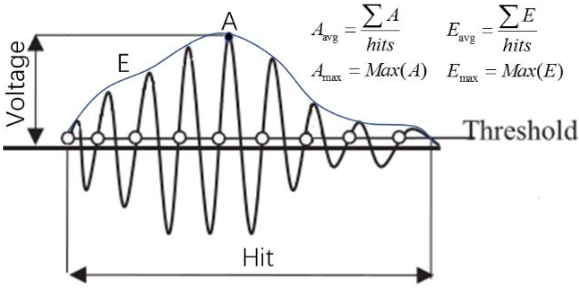
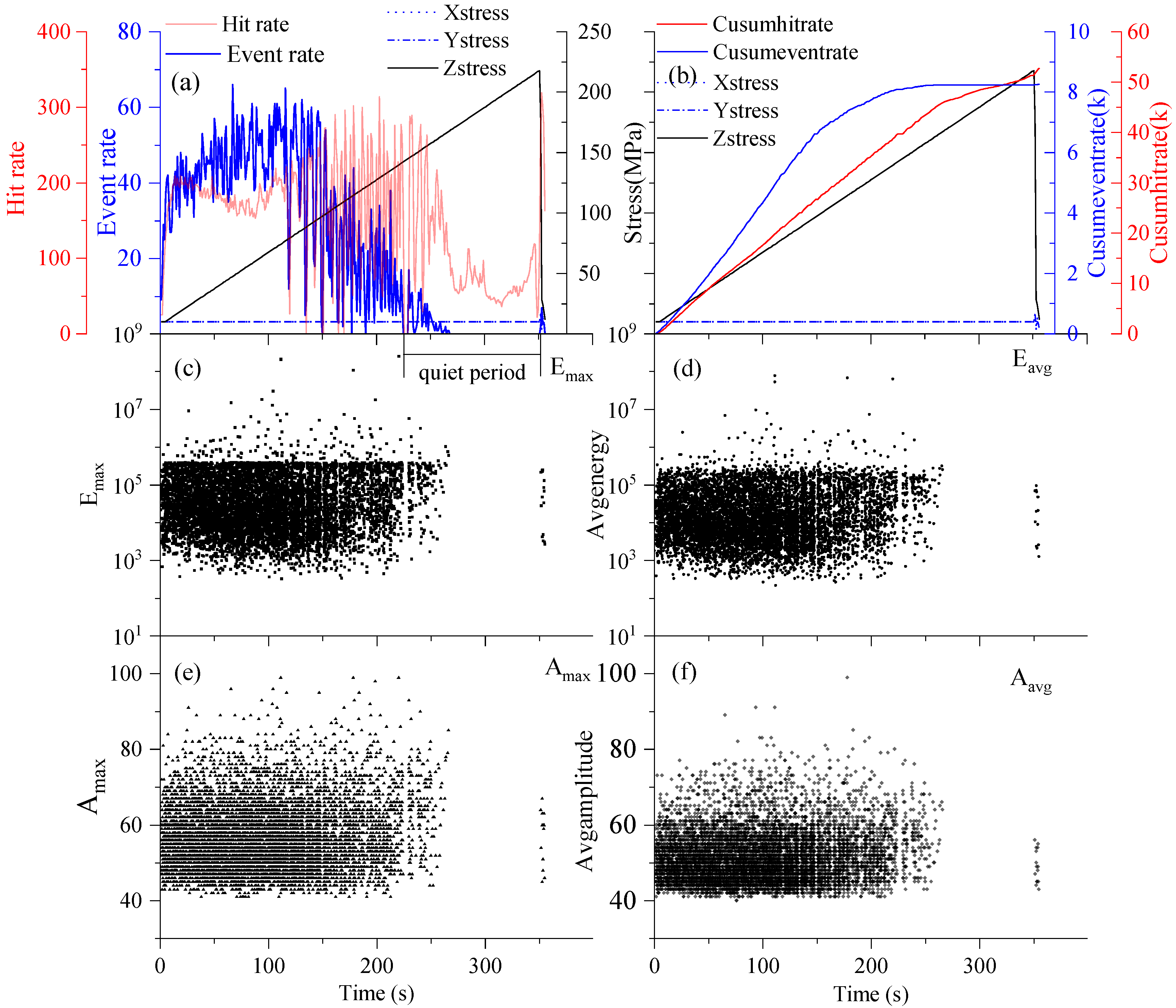
3.2. AE Signals
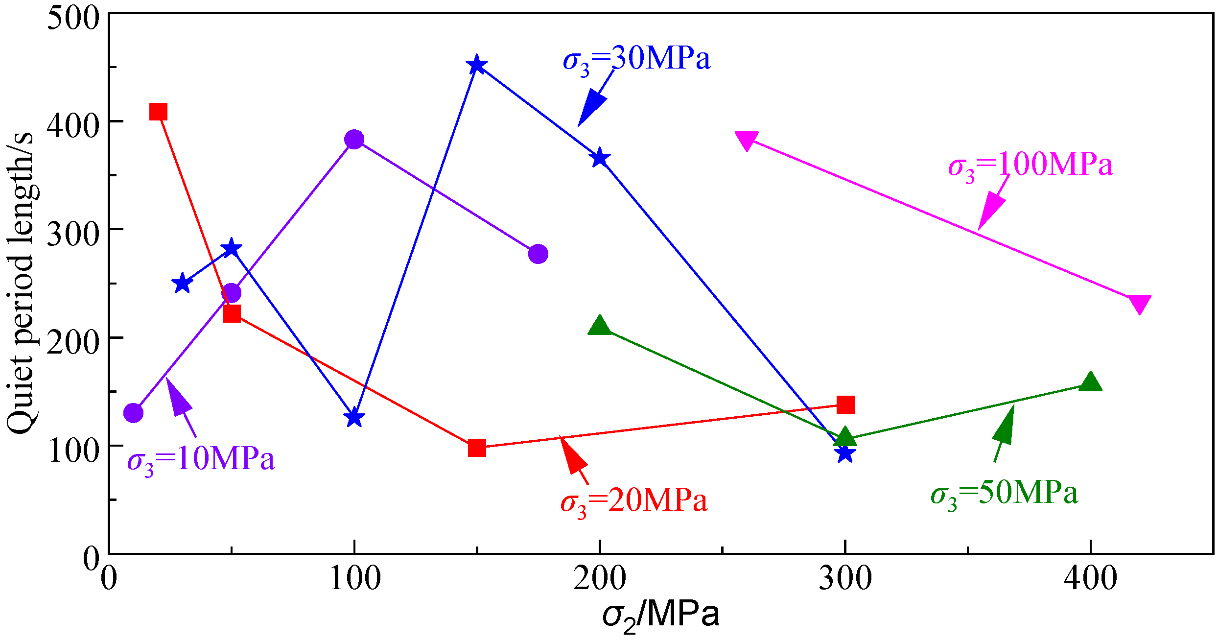
3.3. Quiet Period
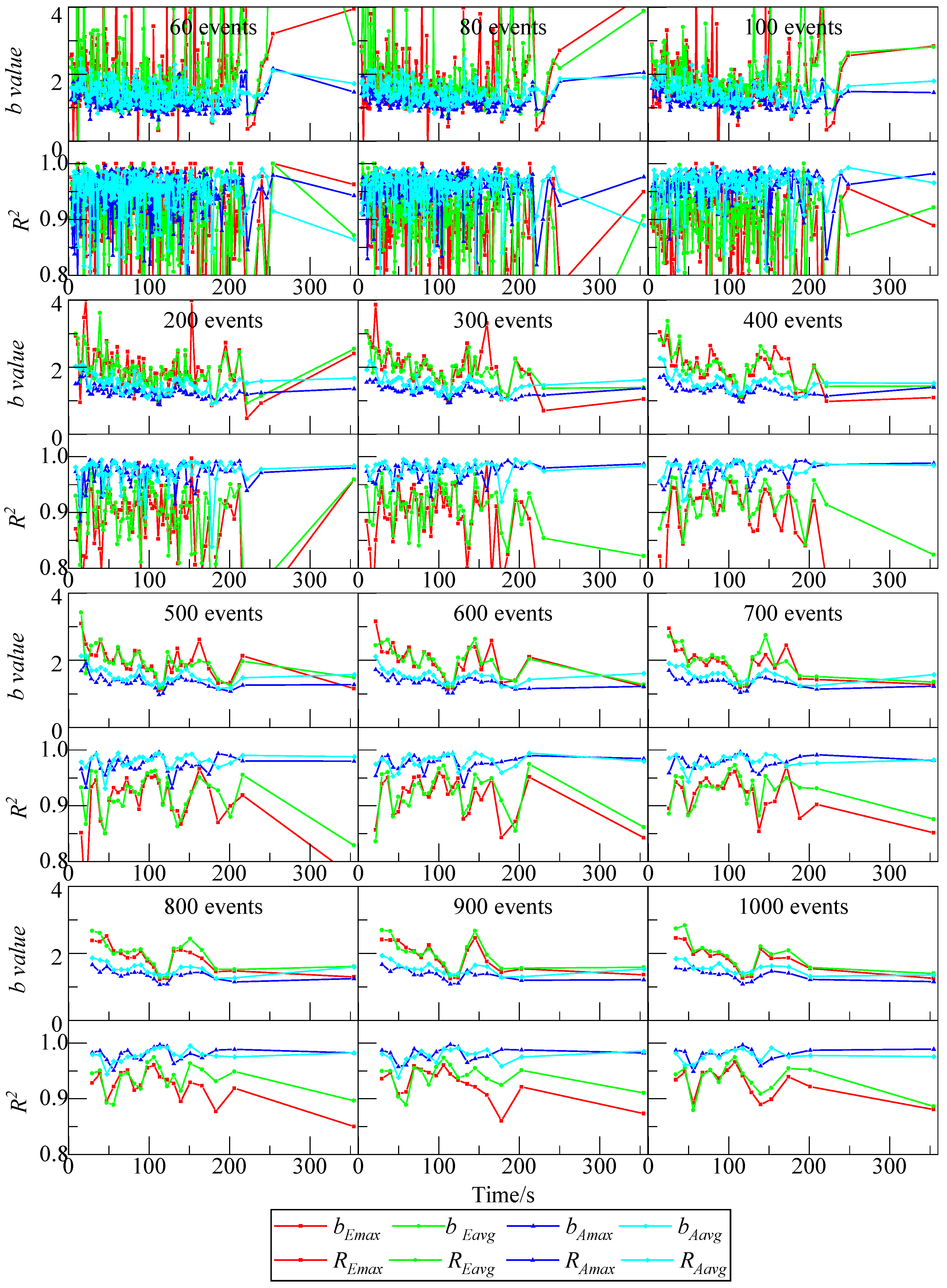
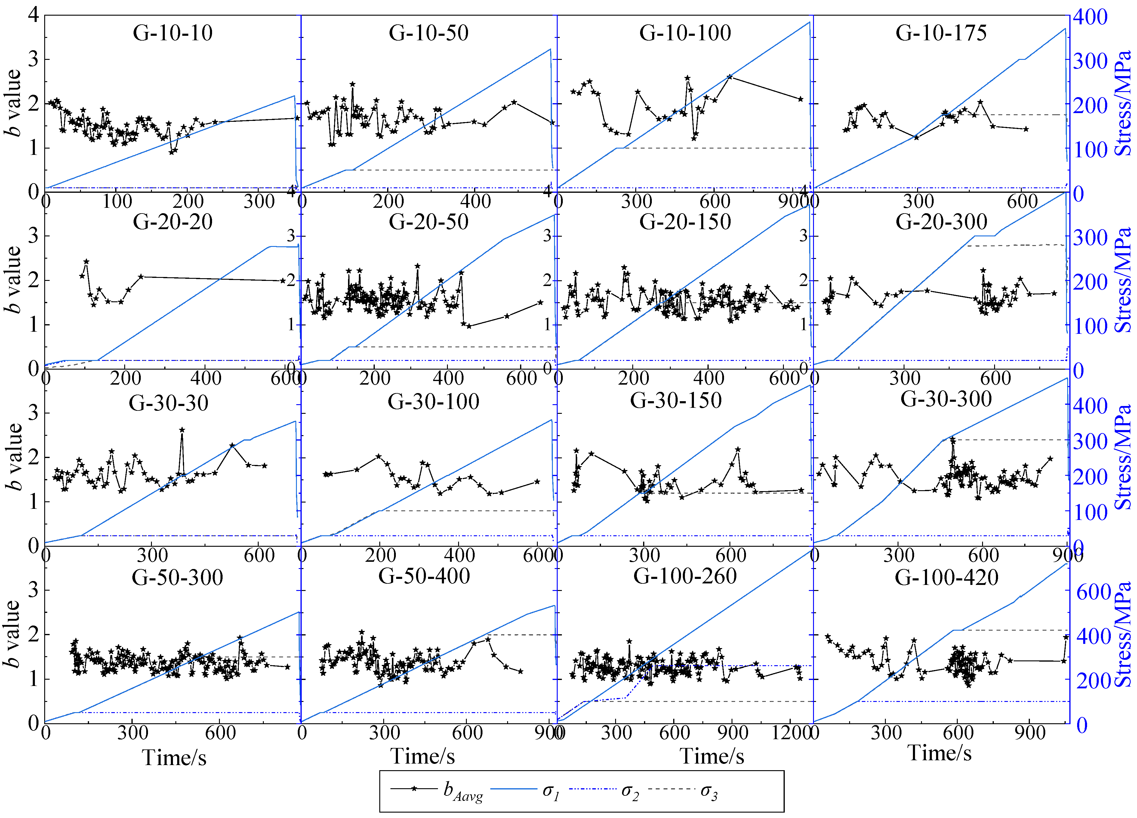
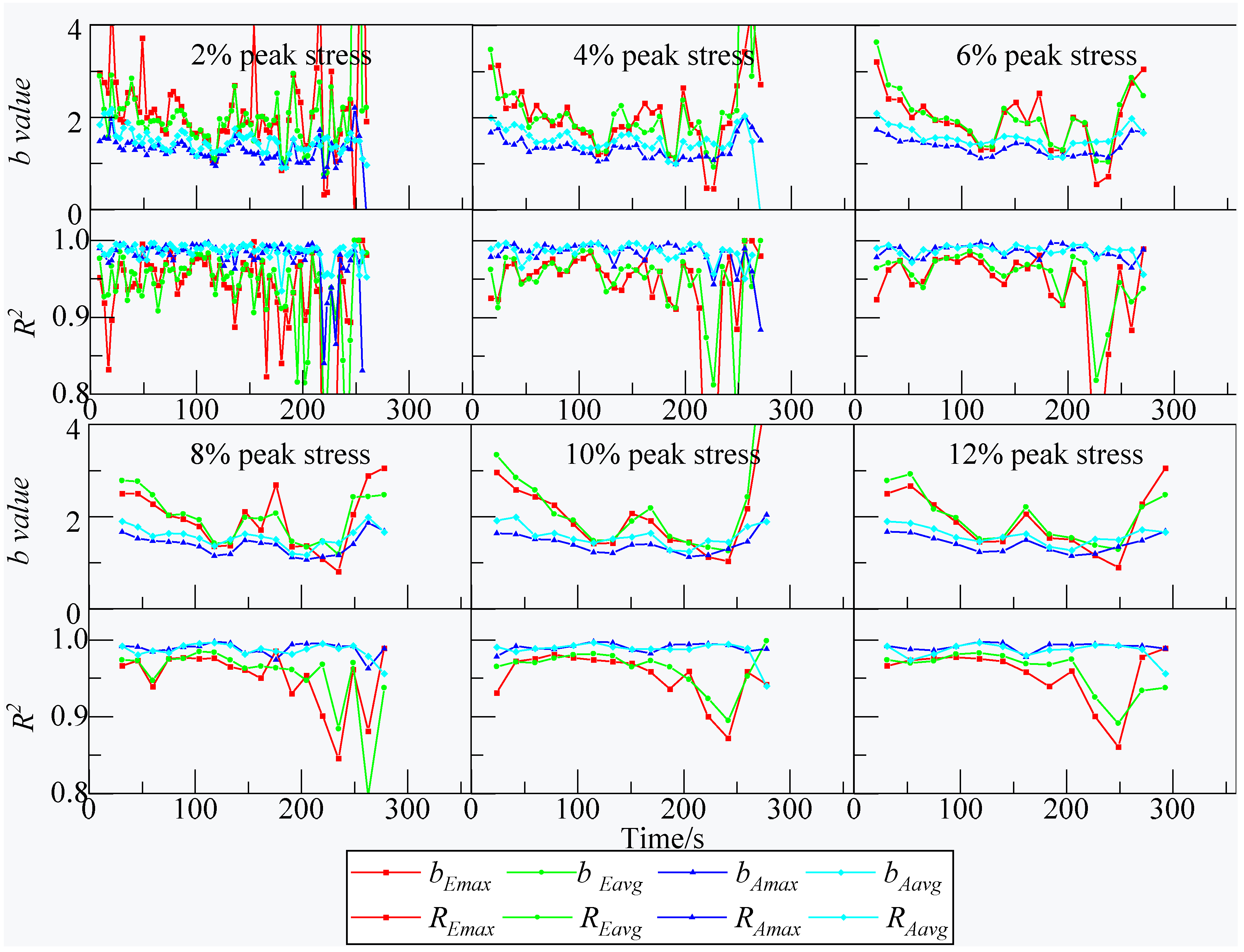
3.4. b Value
4. Conclusions
Author Contributions
Funding
Informed Consent Statement
Data Availability Statement
Conflicts of Interest
Abbreviations
| σ1 | maximum principal stress (MPa) |
| σ2 | intermediate principal stress (MPa) |
| σ3 | minimum principal stress (MPa) |
| Amax | maximum amplitude of an acoustic emission event (dB) |
| Aavg | average amplitude of an acoustic emission event (dB) |
| Emax | maximum absolute energy of an acoustic emission event (aJ) |
| Eavg | average absolute energy of an acoustic emission event (aJ) |
| bA | b value based on the amplitude |
| bE | b value based on the energy |
| bAmax | b value based on the maximum amplitude of multiple hits |
| bAavg | b value based on the average amplitude of multiple hits |
| bEmax | b value based on the maximum energy of multiple hits |
| bEavg | b value based on the average energy of multiple hits |
| R2 | goodness of fitting |
| RAmax | fitting goodness of b value based on the maximum amplitude of multiple hits |
| RAavg | fitting goodness of b value based on the average amplitude of multiple hits |
| REmax | fitting goodness of b value based on the maximum energy of multiple hits |
| REavg | fitting goodness of b value based on the average energy of multiple hits |
References
- Gutenberg, B.; Richter, C.F. Frequency of earthquakes in California. Bull. Seismol. Soc. Am. 1994, 34, 185–188. [Google Scholar] [CrossRef]
- Smith, W.D. The b-value as an earthquake precursor. Nature 1981, 289, 136–139. [Google Scholar] [CrossRef]
- Rao, M.V.M.S.; Lakshmi, K.J.P. Analysis of b-value and improved b-value of acoustic emissions accompanying rock fracture. Curr. Sci. 2005, 89, 1577–1582. [Google Scholar]
- Liu, X.L.; Han, M.S.; He, W.; Li, X.B.; Chen, D.L. A new b-value estimation method in rock acoustic emission testing. J. Geophys. Res. Solid Earth 2020, 125, e2020JB019658. [Google Scholar] [CrossRef]
- Jordan, T.H.; Chen, Y.T.; Gasparini, P.; Madariaga, R.; Main, I.G.; Marzocchi, W.; Papadopoulos, G.; Sobolev, G.; Yamaoka, K.; Zschau, J. Operational earthquake forecasting: State of Knowledge and Guidelines for Utilization. Ann. Geophys. Italy 2011, 54, 361–391. [Google Scholar]
- Sammonds, P.R.; Meredith, P.G.; Main, I.G. Role of pore fluids in the generation of seismic precursors to shear fracture. Nature 1992, 359, 228–230. [Google Scholar] [CrossRef]
- Kwiatek, G.; Goebel, T.H.W.; Dresen, G. Seismic moment tensor and b value variations over successive seismic cycles in laboratory stick-slip experiments. Geophys. Res. Lett. 2014, 41, 5838–5846. [Google Scholar] [CrossRef] [Green Version]
- Goh, A.T.C.; Zhang, W. Reliability assessment of stability of underground rock caverns. Int. J. Rock Mech. Min. Sci. 2012, 55, 157–163. [Google Scholar] [CrossRef]
- Jafari, M.A. The distribution of b-value in different seismic provinces of Iran. In Proceedings of the 14th World Conference on Earthquake Engineering, Beijing, China, 12–17 October 2008. [Google Scholar]
- Okal, E.A.; Romanowicz, B.A. On the variation of b -values with earthquake size. Phys. Earth Planet. Inter. 1994, 87, 55–76. [Google Scholar] [CrossRef]
- Scholz, C.H. Microfractures, aftershocks, and seismicity. Bull. Seismol. Soc. Am. 1968, 58, 1117–1130. [Google Scholar]
- Weeks, J.; Lockner, D.; Byerlee, J. Change in b-values during movement on cut surfaces in granite. Bull. Seismol. Soc. Am. 1978, 68, 333–341. [Google Scholar] [CrossRef]
- Lockner, D.A.; Byerlee, J.D.; Kuksenko, V.; Ponomarev, A.; Sidorin, A. Quasi-static fault growth and shear fracture energy in granite. Nature 1991, 350, 39. [Google Scholar] [CrossRef]
- Mondal, D.; Roy, P. Fractal and seismic b-value study during dynamic roof displacements (roof fall and surface blasting) for enhancing safety in the longwall coal mines. Eng. Geol. 2019, 253, 184–204. [Google Scholar] [CrossRef]
- Liu, X.; Liu, Z.; Li, X.; Gong, F.; Du, K. Experimental study on the effect of strain rate on rock acoustic emission characteristics. Int. J. Rock Mech. Min. Sci. 2020, 133, 104420. [Google Scholar] [CrossRef]
- Wang, S.; Tang, Y.; Wang, S. Influence of brittleness and confining stress on rock cuttability based on rock indentation tests. J. Cent. South Univ. 2021, 28, 2786–2800. [Google Scholar] [CrossRef]
- Lei, X.L. How do asperities fracture? An experimental study of unbroken asperities. Earth Planet. Sci. Lett. 2003, 213, 347–359. [Google Scholar] [CrossRef]
- Main, I.G.; Meredith, P.G.; Jones, C. A reinterpretation of the precursory seismic b-value anomaly from fracture mechanics. Geophys. J. Int. 1989, 96, 131–138. [Google Scholar] [CrossRef]
- Main, I.G.; Sammonds, P.R.; Meredith, P.G. Application of a modified Griffith criterion to the evolution of fractal damage during compressional rock failure. Geophys. J. Int. 1993, 115, 367–380. [Google Scholar] [CrossRef] [Green Version]
- Schroeder, M. Fractals, Chaos, Power Laws: Minutes From an Infinite Paradise. Phys. Today 1991, 44, 91. [Google Scholar] [CrossRef]
- Clauset, A.; Shalizi, C.R.; Newman, M.E.J. Power-Law Distributions in Empirical Data. Siam Rev. 2009, 51, 661–703. [Google Scholar] [CrossRef] [Green Version]
- Mogi, K. Study of elastic shocks caused by the fracture of heterogeneous materials and its relation to earthquake phenomena. Bull. Earthq. Res. Inst. Univ. Tokyo 1962, 40, 125–173. [Google Scholar]
- Scholz, C. The frequency-magnitude relation of microfracturing in rock and its relation to earthquakes. Bull. Seismol. Soc. Am. 1968, 58, 399–415. [Google Scholar] [CrossRef]
- Zitto, M.E.; Piotrkowski, R.; Gallego, A.; Sagasta, F.; Benavent-Climent, A. Damage assessed by wavelet scale bands and b-value in dynamical tests of a reinforced concrete slab monitored with acoustic emission. Mech. Syst. Signal Process. 2015, 60–61, 75–89. [Google Scholar] [CrossRef]
- Sagasta, F.; Zitto, M.E.; Piotrkowski, R.; Benavent-Climent, A.; Suarez, E.; Gallego, A. Acoustic emission energy b-value for local damage evaluation in reinforced concrete structures subjected to seismic loadings. Mech. Syst. Signal Process. 2018, 102, 262–277. [Google Scholar] [CrossRef]
- Wiemer, S.; Katsumata, K. Spatial variability of seismicity parameters in aftershock zones. J. Geophys. Res. 1999, 104, 13135–13151. [Google Scholar] [CrossRef]
- Wiemer, S.; Wyss, M. Minimum magnitude of completeness in earthquake catalogs: Examples from Alaska, the western United States, and Japan. Bull. Seismol. Soc. Am. 2000, 90, 859–869. [Google Scholar] [CrossRef]
- Cao, A.; Gao, S.S. Temporal variation of seismic b-values beneath northeastern Japan island arc. Geophys. Res. Lett. 2002, 29, 48-1–48-3. [Google Scholar] [CrossRef]
- Woessner, J.; Wiemer, S. Assessing the quality of earthquake catalogues: Estimating the magnitude of completeness and its uncertainty. Bull. Seismol. Soc. Am. 2005, 95, 684–698. [Google Scholar] [CrossRef]
- Dong, L.; Li, X.; Tang, L.; Gong, F. Mathematical Functions and Parameters for Microseismic Source Location without Pre-Measuring Speed. Chin. J. Rock Mech. Eng. 2011, 30, 2057–2067. [Google Scholar]
- Kda, B.; Cy, A.; Rui, S.A.; Ming, T.A.; Sw, A. Failure properties of cubic granite, marble, and sandstone specimens under true triaxial stress. Int. J. Rock Mech. Min. Sci. 2020, 130, 104309. [Google Scholar]
- Du, K.; Tao, M.; Li, X.B.; Zhou, J. Experimental Study of Slabbing and Rockburst Induced by True-Triaxial Unloading and Local Dynamic Disturbance. Rock Mech. Rock Eng. 2016, 49, 3437–3453. [Google Scholar] [CrossRef]
- Luo, Y.; Gong, F.; Liu, D.; Wang, S.; Si, X. Experimental simulation analysis of the process and failure characteristics of spalling in d-shaped tunnels under true-triaxial loading conditions. Tunn. Undergr. Space Technol. 2019, 90, 42–61. [Google Scholar] [CrossRef]
- Gong, F.Q.; Si, X.F.; Li, X.B.; Wang, S.Y. Experimental investigation of strain rockburst in circular caverns under deep three-dimensional high-stress conditions. Rock Mech. Rock Eng. 2019, 52, 1459–1474. [Google Scholar] [CrossRef]
- Wang, S.; Sun, L.C.; Li, X.; Wang, S.; Feng, F. Experimental investigation of cuttability improvement for hard rock fragmentation using conical cutter. Int. J. Geomech. 2020, 21, 06020039. [Google Scholar] [CrossRef]
- Nur, A.; Simmons, G. Stress-induced velocity anisotropy in rock: An experimental study. J. Geophys. Res. 1969, 74, 6667–6674. [Google Scholar] [CrossRef]
- Qi-Yue, L.I.; Dong, L.J.; Xi-Bing, L.I.; Yin, Z.Q.; Liu, X.L. Effects of Sonic Speed on Location Accuracy of Acoustic Emission Source in Rocks. Trans. Nonferrous Met. Soc. China 2011, 21, 2719–2726. [Google Scholar]
- Dong, L.J.; Tao, Q.; Qing-Chun, H.U. Influence of temperature on acoustic emission source location accuracy in underground structure. Trans. Nonferrous Met. Soc. China 2021, 31, 2468–2478. [Google Scholar] [CrossRef]
- Dong, L.; Zou, W.; Li, X.; Shu, W.; Wang, Z. Collaborative Localization Method Using Analytical and Iterative Solutions for Microseismic/Acoustic Emission Sources in the Rockmass Structure for Underground Mining. Eng. Fract. Mech. 2019, 210, 95–112. [Google Scholar] [CrossRef]
- Dong, L.J.; Tang, Z.; Li, X.B.; Chen, Y.C.; Xue, J.C. Discrimination of mining microseismic events and blasts using convolutional neural networks and original waveform. J. Cent. South Univ. 2020, 27, 3078–3089. [Google Scholar] [CrossRef]
- Dong, L.; Tong, X.; Hu, Q.; Tao, Q. Empty region identification method and experimental verification for the two-dimensional complex structure. Int. J. Rock Mech. Min. Sci. 2021, 147, 104885. [Google Scholar] [CrossRef]
- Dong, L.; Tong, X.; Ma, J. Quantitative investigation of tomographic effects in abnormal regions of complex structures. Engineering 2021, 7, 1011–1022. [Google Scholar] [CrossRef]
- Dong, L.J.; Li, X.B.; Zhou, Z.L.; Chen, G.H.; Ma, J. Three-dimensional analytical solution of acoustic emission source location for cuboid monitoring network without pre-measured wave velocity. Trans. Nonferrous Met. Soc. China 2015, 25, 293–302. [Google Scholar] [CrossRef]
- Dong, L.; Shu, W.; Li, X.; Han, G.; Wei, Z. Three dimensional comprehensive analytical solutions for locating sources of sensor networks in unknown velocity mining system. IEEE Access 2017, 5, 11337–11351. [Google Scholar] [CrossRef]
- Dong, L.; Sun, D.; Li, X.; Du, K. Theoretical and experimental studies of localization methodology for AE and microseismic sources without pre-measured wave velocity in mines. IEEE Access 2017, 5, 16818–16828. [Google Scholar] [CrossRef]
- Dong, L.; Hu, Q.; Tong, X.; Liu, Y. Velocity-free ms/ae source location method for three-dimensional hole-containing structures. Engineering 2020, 6, 827–834. [Google Scholar] [CrossRef]
- Chen, D.; Liu, X.; He, W.; Xia, C.; Gong, F.; Li, X.; Cao, X. Effect of attenuation on amplitude distribution and b value in rock acoustic emission tests. Geophys. J. Int. 2021. [Google Scholar] [CrossRef]
- Du, K.; Su, R.; Tao, M.; Yang, C.; Momeni, A.; Wang, S. Specimen shape and cross-section effects on the mechanical properties of rocks under uniaxial compressive stress. Bull. Eng. Geol. Environ. 2019, 78, 6061–6074. [Google Scholar] [CrossRef]


| Specimen No. | ST | ET | ST/ET | DT | σ1qp/MPa | σ1max/MPa | σ1qp/σ1max |
|---|---|---|---|---|---|---|---|
| G-10-10 | 226 | 356 | 0.37 | 130 | 142.35 | 217.90 | 0.65 |
| G-10-50 | 334 | 575 | 0.42 | 241 | 186.21 | 323.00 | 0.58 |
| G-10-100 | 583 | 966 | 0.40 | 383 | 231.51 | 351.00 | 0.66 |
| G-10-175 | 450 | 727 | 0.38 | 277 | 213.91 | 370.00 | 0.58 |
| G-20-20 | 224 | 633 | 0.65 | 409 | 75.12 | 293.20 | 0.26 |
| G-20-50 | 470 | 692 | 0.32 | 222 | 242.90 | 348.40 | 0.70 |
| G-20-150 | 571 | 669 | 0.15 | 98 | 325.16 | 390.00 | 0.83 |
| G-20-300 | 699 | 837 | 0.16 | 138 | 344.18 | 399.03 | 0.86 |
| G-30-30 | 455 | 705 | 0.35 | 250 | 236.66 | 353.39 | 0.67 |
| G-30-50 | 387 | 669 | 0.42 | 282 | 197.17 | 340.69 | 0.58 |
| G-30-100 | 510 | 636 | 0.20 | 126 | 281.73 | 357.33 | 0.79 |
| G-30-150 | 427 | 879 | 0.51 | 452 | 224.36 | 455.17 | 0.49 |
| G-30-200 | 586 | 952 | 0.38 | 366 | 307.85 | 500.21 | 0.62 |
| G-30-300 | 808 | 901 | 0.10 | 93 | 437.32 | 474.57 | 0.92 |
| G-50-200 | 773 | 982 | 0.21 | 209 | 409.69 | 535.07 | 0.77 |
| G-50-300 | 767 | 873 | 0.12 | 106 | 439.68 | 503.08 | 0.87 |
| G-50-400 | 764 | 921 | 0.17 | 157 | 458.77 | 532.66 | 0.86 |
| G-100-260 | 919 | 1303 | 0.29 | 384 | 548.55 | 750.00 | 0.73 |
| G-100-420 | 821 | 1054 | 0.22 | 233 | 538.00 | 815.00 | 0.66 |
| AE Event Interval | Mean of REmax | Mean of REavg | Mean of RAmax | Mean of RAavg |
|---|---|---|---|---|
| 60 | 0.890 | 0.902 | 0.945 | 0.945 |
| 80 | 0.883 | 0.900 | 0.955 | 0.954 |
| 100 | 0.879 | 0.892 | 0.959 | 0.960 |
| 200 | 0.881 | 0.895 | 0.968 | 0.971 |
| 300 | 0.888 | 0.910 | 0.973 | 0.977 |
| 400 | 0.897 | 0.917 | 0.974 | 0.978 |
| 500 | 0.905 | 0.917 | 0.974 | 0.980 |
| 600 | 0.916 | 0.923 | 0.976 | 0.980 |
| 700 | 0.920 | 0.929 | 0.979 | 0.979 |
| 800 | 0.923 | 0.935 | 0.979 | 0.978 |
| 900 | 0.926 | 0.939 | 0.980 | 0.976 |
| 1000 | 0.927 | 0.935 | 0.980 | 0.977 |
| Stress Proportion Interval | Mean of REmax | Mean of REavg | Mean of RAmax | Mean of RAavg |
|---|---|---|---|---|
| 2% | 0.867 | 0.875 | 0.955 | 0.971 |
| 4% | 0.883 | 0.896 | 0.970 | 0.973 |
| 6% | 0.887 | 0.907 | 0.973 | 0.974 |
| 8% | 0.904 | 0.909 | 0.977 | 0.973 |
| 10% | 0.906 | 0.928 | 0.980 | 0.974 |
| 12% | 0.914 | 0.919 | 0.982 | 0.971 |
| Stress Interval/MPa | Mean of REmax | Mean of REavg | Mean of RAmax | Mean of RAavg |
|---|---|---|---|---|
| 5 | 0.859 | 0.882 | 0.967 | 0.971 |
| 10 | 0.878 | 0.904 | 0.967 | 0.973 |
| 15 | 0.897 | 0.898 | 0.972 | 0.970 |
| 20 | 0.912 | 0.927 | 0.970 | 0.978 |
| 25 | 0.908 | 0.909 | 0.981 | 0.976 |
| 30 | 0.907 | 0.913 | 0.982 | 0.975 |
Publisher’s Note: MDPI stays neutral with regard to jurisdictional claims in published maps and institutional affiliations. |
© 2022 by the authors. Licensee MDPI, Basel, Switzerland. This article is an open access article distributed under the terms and conditions of the Creative Commons Attribution (CC BY) license (https://creativecommons.org/licenses/by/4.0/).
Share and Cite
Dong, L.; Zhang, L.; Liu, H.; Du, K.; Liu, X. Acoustic Emission b Value Characteristics of Granite under True Triaxial Stress. Mathematics 2022, 10, 451. https://doi.org/10.3390/math10030451
Dong L, Zhang L, Liu H, Du K, Liu X. Acoustic Emission b Value Characteristics of Granite under True Triaxial Stress. Mathematics. 2022; 10(3):451. https://doi.org/10.3390/math10030451
Chicago/Turabian StyleDong, Longjun, Lingyun Zhang, Huini Liu, Kun Du, and Xiling Liu. 2022. "Acoustic Emission b Value Characteristics of Granite under True Triaxial Stress" Mathematics 10, no. 3: 451. https://doi.org/10.3390/math10030451
APA StyleDong, L., Zhang, L., Liu, H., Du, K., & Liu, X. (2022). Acoustic Emission b Value Characteristics of Granite under True Triaxial Stress. Mathematics, 10(3), 451. https://doi.org/10.3390/math10030451