1. Introduction
The geological interpretation of polylines produced by geological logging in the process of exploration and production is more complex than the interpretation of polylines produced by drilling in geological explorations [
1]. In this case, the efficiency will be very low if the model is constructed by the contour triangulation method [
2] that uses triangulation for surface reconstruction. Moreover, exploration and production are carried out during the operation of the mine, which leads to the result that the traditional modeling methods cannot keep up with the mining plan. Modeling is the basis and premise of mine digital production [
3]. Efficient real-time modeling is of great significance for mine production and promoting the development of mine digital construction. The method we proposed can slightly process the geological interpretation polylines to carry out automatic implicit modeling, which greatly improves the modeling efficiency and quality.
In recent years, there has been great progress in both theory and methodology of implicit modeling. A range of implicit modeling methods based on different interpolation functions and geological rules have been proposed [
4,
5,
6,
7,
8]. The key to implicit orebody modeling is to figure out how to interpolate the unknown 3D orebody model based on the limited geological sampling data. For the complex geological sampling data, the quality of implicit modeling results largely depends on the reliability of constructed constraints. We attempt to solve the problem of normal estimation based on cross-contour polylines (non-parallel geological interpretation polylines) to improve the automation of implicit orebody modeling.
For two kinds of common geological sampling data, drillhole data and geological interpretation polylines, the implicit modeling methods based on them require estimating their normals. The implicit equation is solved based on the estimated normals. The implicit surface reconstruction is carried out based on the solved implicit equation. The research results of normal estimation for dense point clouds are considered relatively mature [
9,
10,
11,
12]. Generally speaking, they can be divided into three categories: the method based on the local plane fitting method first proposed by Hoppe et al. [
9], the method based on Delaunay/Voronoi first proposed by Amenta et al. [
10], and the method based on robust statistics [
11]. Compared with the point cloud, cross-contour polylines are more difficult to estimate the normals because of their more complex topological adjacency relationships [
13].
However, there have been many existing studies on the 3D modeling of directed contours. Shao et al. [
14] estimated the normals of the cross-section contours and the surface of the object in the design drawing, then reconstructed the surface to model the design sketch in 3D. Firstly, they proposed a method to estimate the normals of the cross-section contours and found a clear mathematical formula between the cross-section contours and the geometric relationship they convey. Secondly, they used this relationship to realize the algorithm of object surface reconstruction. The limitation of this method is that it is only suitable for constructing the model by normal estimation of the cross-section contours. Park et al. [
15] estimated the normal vectors of the 3D curves by a new algorithm. In addition, they established an optimization equation that can reflect the design intention. Through the above two steps, a model with insufficient geometric information can be constructed. Kniss et al. [
16] described the concept of multi-dimensional transfer functions in detail and used the functions to form a new technique for interactively constructing the surface of the object. Ijiri et al. [
17] improved the traditional methods [
18,
19] and proposed Bilateral Hermite Radial Basis Functions for Contour-based Volume Segmentation. In addition, they also proposed a cyclic LU decomposition scheme to accelerate B-HRBF calculation, which realized real-time and intuitive volume segmentation of real object images. However, it is difficult for novices to accurately place the cross-section to specify the contour of segmentation, which will affect the effect of segmentation. Zhong et al. [
20] proposed an improved method to reconstruct the orebody surface from a set of interpreted cross-sections. Moreover, they also proposed an iterative closest point correction algorithm, which can iteratively correct the distance field according to the constraint rules and the internal and external position relationship of the model. However, this method is only applicable to non-trivial and non-sparse areas of data
In the absence of prior contour polyline information, although various normal estimation methods have been proposed, it is still difficult to accurately estimate the real normals of cross-contour polylines due to the sparsity of sampling data.
In this work, we consider transforming the problem of orebody modeling based on non-parallel geological interpretation polylines in geological modeling into the problem of normal estimation of cross-contour polylines. Because geological interpretation polylines produced by geological logging in the process of exploration and production have a complex adjacency relationship, it is generally difficult to satisfy the requirements of orebody modeling using the normals obtained by the traditional normal estimation methods. On the one hand, the normal estimation of cross-contour polylines should consider more topological adjacency than that of parallel contours to obtain more accurate normal estimation results. On the other hand, the traditional method of normal estimation of contour polylines based on a single polyline is not suitable for the normal estimation of cross- contour polylines. Moreover, it is also difficult to estimate the normals of cross-contour polylines by the manual interaction method. As a result, it is necessary to provide an automatic normal estimation method of cross-contour polylines to improve the efficiency of implicit orebody modeling.
Because the adjacent segments at an intersection point have strong topological correlation characteristics and satisfy the conditions of the local fitting plane, we considered using the least square plane fitting method based on principal component analysis (PCA) to estimate the normal of cross-contour polylines. Inspired by the point cloud normal estimation strategy, we consider the normalized line segments endpoints in the intersection point neighborhood as a point cloud and use the PCA method to estimate the normal of the intersection point. Then, according to the geometric relationship, the normals of the beginning and the end segments of the corresponding polyline are estimated. Next, the normals of middle line segments are estimated using the linear interpolation method. After that, reorient the normal direction of all cross-contour polylines through the method based on the normal propagation.
After determining the normals of the contour polylines, we can use the implicit modeling [
21,
22,
23,
24] method based on radial basis function interpolation [
25,
26,
27,
28,
29,
30,
31,
32] to carry out 3D orebody modeling. To interpolate the directed contour polylines, firstly, we obtain the on-surface interpolation constraints by sampling contour polylines. Secondly, the off-surface interpolation constraints are constructed according to the idea of signed distance field [
33,
34,
35,
36,
37] and the way of adaptively offsetting sampling points. Finally, the radial basis function interpolation method is used to interpolate the corresponding constraints to obtain the implicit function representing the orebody model, and the implicit surface reconstruction method [
38,
39,
40,
41,
42,
43] is used to extract the isosurfaces.
The method we propose is based on the basic assumption that several segments connected to the intersection points of contour polylines satisfy the characteristics of local curvature. It is suitable for both the planar cross-contour polylines and non-planar cross- contour polylines. However, it requires that line segments must strictly intersect at points and can be interrupted at the points. In summary, we present an innovative method for normal estimation of cross-contour polylines and an innovative method for reorienting normal directions.
2. Method
The basic idea of normal estimation of cross-contour polylines in orebody modeling is to construct a virtual network using the orebody cross contour polylines obtained by geological interpretation, and then the normals of the cross-contour polylines can be estimated and reoriented.
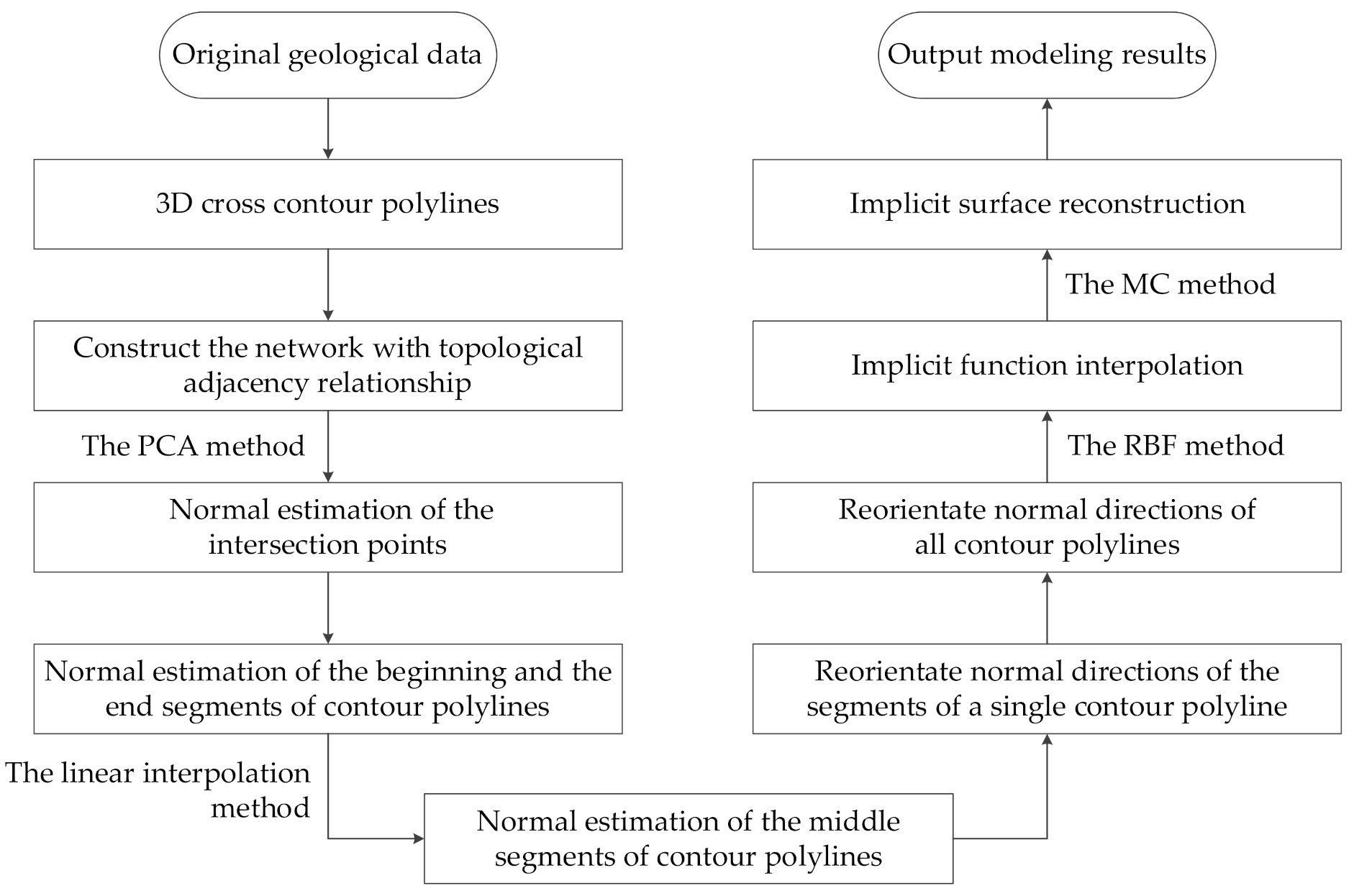
Figure 1 shows the overall process of the method, which mainly consists of the following three steps:
- (1)
According to the orebody cross-contour polylines obtained by geological interpretation in the process of exploration and production, a virtual network is constructed to determine the topological adjacency relationship of contour polylines and the corresponding intersection points. Next, the endpoints of the normalized line segments connected to the intersection points are regarded as point clouds, and the normals at the intersection points are obtained by using the method based on local plane fitting. Then, according to the spatial geometric relationship, the estimated normals of the beginning and the end segments of the contour polylines can be obtained. At last, the normals of the middle segments of the contour polylines can be estimated by the way of linear interpolation. Based on the above steps, we can obtain the unoriented normals of all contour polylines.
- (2)
The contour interpolation method requires that the normal directions of the contour polylines be consistent, so this stage is divided into two steps to realize it. Firstly, starting from one end of a contour polyline, the judgment vectors are obtained by cross multiplication of the direction vector projection and the normal vector of adjacent line segments. Then the point multiplication result of judgment vectors is used to adjust the normal directions of segments. Therefore, we can reorient the normal directions of a single contour polyline. Secondly, we can flip the normals of the polylines by comparing the normals of the adjacent line segments at each intersection points. Finally, the normal propagation method can be used to realize the normal direction reorientation of all polylines.
- (3)
Calculate the implicit function representing the orebody model by using the radial basis function interpolation method and extract the isosurface by the marching cubes (MC) method. Finally, we can obtain the orebody model.
2.1. Normal Estimation
According to the above general idea, to estimate the normal vectors of the cross-contour polylines, first, we should estimate the normals of the intersection points. The foundation of this step is to build a virtual network based on topological adjacency of the orebody contour polylines.
2.1.1. Construct the Network of Cross Contours
To construct a virtual network with topological adjacency relationship, we should preprocess the cross-contour polylines of the orebody (the polylines should be broken at intersection points exactly). The constructed virtual network is shown in
Figure 2.
2.1.2. Normal Estimation of the Intersection Points
Based on the normal estimation strategy of point clouds, we believe that the endpoints of the beginning segments connected to the intersection point of the contour polylines can be regarded as a point cloud. Based on the method of local plane fitting, the PCA method is used to estimate the normal of the intersection point. However, due to the different lengths of the line segments connected to the intersection point, they have different effect on the normal estimation. Normalization is carried out in this paper to ensure that the contribution of each segment for the normal estimation is same. The normalized segments can be obtained by clipping the original adjacent line segments using the unit length. And the least square plane of the intersection point can be solved by the endpoints of the normalized line segments (normalized neighborhood points). Based on the fitted plane, we can estimate the normal
of the intersection point:
Here,
represents the number of the normalized neighborhood points;
represents the estimated normal of the intersection point;
represents a normalized neighborhood point. In general, the point
can be calculated as the center of the normalized neighborhood points:
After the above steps, the objective function is:
The final form of the objective function is:
The eigenvalue decomposition of matrix
is carried out, and the eigenvector corresponding to the smallest eigenvalue is the normal vector
of the intersection point to be solved, as shown in
Figure 3.
When an intersection point is only connected to two polylines (that is, the segments connected with the intersection point are not collinear), there are only two normalized neighborhood points, and the least squares plane cannot be solved. In this case, the intersection point and two normalized neighborhood points may be combined to solve the least square plane, and then the normal of the intersection point can be estimated.
It is worth noting that in some special cases, there is no unique solution to the equation and it is impossible to estimate the normal of the intersection point. For example, when an intersection point is only connected with two polylines and the two segments connected with the intersection point are collinear, the least squares plane cannot be solved.
2.1.3. Normal Estimation of the Beginning and the End Segments
We use the normal
of the intersection point estimated in the previous steps to estimate the normals of the beginning and the end segments of a polyline, as shown in
Figure 4. Set the direction vector of the segment connected to the intersection point as
. If two vectors are perpendicular, their vector product is zero. Based on this fact, calculate normal vector
of the plane where
and
are located:
Then, we calculate the normal vector
of the plane where
and
are located.
is the estimated normal of the segment connected to the intersection point of the polyline:
2.2. Linear Interpolation
After the above steps, we can estimate the normals of all segments connected to the intersection points. Based on the estimated normals, we can interpolate the normals of the middle segments of the polyline using the linear interpolation method, as shown in
Figure 5.
For most contour polylines connected with the intersection points, we can obtain the estimated normal of their beginning and the end segments. In this case, we can use the linear interpolation method based on the normals of the beginning and the end segments to interpolate the normals of the middle segments of the polyline.
The normal vectors of the middle segments are affected by both the normal vectors of the beginning and the end segments and the direction vectors of themself. Therefore, in this paper, based on the normal vectors of the beginning and the end segments, we interpolate the tangent vectors instead of the normal vectors of the line segments. Set the direction vector and normal vector of one segment connected to the intersection point of the polyline as
and
. Then, we can calculate the tangent vector of the line segment:
Setting the direction vector and normal vector of the other segment connected to the intersection point of the polyline as
and
, then, we can calculate the tangent vector of line segment:
If:
then we flip the tangent vector
to ensure the reliability of linear interpolation results.
Set the tangent vector of segment
of the polyline as
, direction vector as
, normal vector as
.
represents the online distance between
and
.
represents the online distance between
and
:
where:
Then, based on the tangent vector, we can calculate the normal vector:
The normal direction of the whole polyline can be interpolated one by one. It is worth noting that for the polylines near the boundary of the cross-contour of the orebody and the polylines at some special positions, which have only one segment connected to the intersection point, they have only one estimated normal. For these polylines, the normals of the middle segments should be interpolated in another way.
Firstly, based on the known normal vector of the segment connected to the intersection point, calculate the tangent vector. Set the direction vector of this segment as
, normal vector as
. Then, we can calculate the tangent vector
:
Secondly, interpolation is carried out with 1 as the weight. It is assumed that the tangent vectors of all segments of the whole polyline are
. Set the direction vector of segment
of the polyline as
, normal vector as
:
2.3. Reorient Normal Directions
The normal vectors of all line segments can be estimated based on the above steps, but their directions may be inconsistent. To interpolate the contour polylines using the implicit modeling method, it is necessary to reorient the normal directions. Our idea is to make the normal directions of an initial polyline consistent first. Then the normal directions of multiple polylines adjacent to the intersection are reoriented. Finally, the normal directions of all polylines can be reoriented by using the normal propagation method.
2.3.1. Reorient Normal Directions of a Single Contour Polyline
Set the segments of a polyline in the cross-contour network as
,
direction vector of them as
,
normal vector as
,
. The tangent plane of
is
. The tangent plane of
is
. Plane
is perpendicular to
and
, and the intersection point of
and
is on it, as shown in
Figure 6.
The projection vector
and
are calculated by projecting the vector
and
into the plane
. Then, we can calculate the vector
and
as judgment vectors:
If:
then we flip
.
If:
then we retain the original orientation.
It should be noted that when and are coplanar, the above method is not applicable. In this case, the normal vectors and of line segments are directly used as the judgment vectors. Then we can calculate the sign of point multiplication to judge whether the normal directions are consistent.
2.3.2. Reorient Normal Directions of Multiple Contour Polylines
Based on the above steps, the normal directions of single one polyline are consistent, but the normal directions may not be consistent between polylines. By calculating the sign of the normal vectors of the intersection point and the connected segments, the orientations of the normal vectors can be reoriented, as shown in
Figure 7.
Set the estimated normal vector at an intersection in the cross-contour network as , the estimated normal vector of the segments connected to it as , :
If:
then we flip the normal vectors of the polyline where the segment
is located.
If:
then we retain the original orientation.
Based on the network of the cross-contour polylines, the normal propagation method is used to reorient normal directions of all polylines. To accelerate the speed of the reorientation process, the topological adjacency relationship between contour polylines and their intersection points in the network can be constructed in advance. Similar to the process of normal propagation of the point cloud, the breadth-first search (BFS) method is used to traverse each intersection point. According to the above correction formula, reorient the normal directions of the polylines connected to the intersection points. After determining the normals of the contour polylines, we can directly use the implicit modeling method based on RBF to reconstruct the orebody automatically.
2.4. Experiment Information
We implemented the algorithm of the proposed method using the C++ programming language and tested it on a Windows 64-bit computer equipped with a 3.70 GHz Intel (R) Core (TM) i7-8700U processor, 32 GB RAM, and an NVIDIA GeForce RTX 2080 GPU.
To make the experiments scientific and reasonable, we extract the experimental data from the real data obtained in the process of exploration and production of an actual metal mine. The experimental data is divided into four groups with different numbers of intersections and polylines. In order to verify the reliability of the proposed method, the experiment results of the first set data are compared with the results of explicit modeling using the same data.
3. Results and Discussion
We test the normal estimation method on four sets of cross-contour polylines data. These examples are taken from real geological data and obtained from geological logging during the process of exploration and production. The following experimental results clearly show the process of normal estimation, normal reorientation and implicit modeling of the original cross contour polylines step by step, as shown in
Figure 8,
Figure 9,
Figure 10,
Figure 11 and
Figure 12.
3.1. Examples
Figure 8 shows the normal estimation process and results as well as modeling results of the first set of cross-contour polylines.
Figure 8a is the original cross-contour polylines of the orebody. After processing, a network
Figure 8b with the topological adjacency relationship is constructed. The normals of each intersection point are estimated by using the method based on local plane fitting. As shown in
Figure 8c, the green lines represent the estimated normals of intersection points. According to the spatial geometric relationship, the beginning and the end segments of the contour polylines can be estimated. As shown in
Figure 8d, the red surface is the tangent plane of the line segment, the green surface and the blue surface represent the normals of the line segment. The blue surface points to the inside of the model and the green points to the opposite. As shown in
Figure 8e, the normals of the middle segments of the contour polylines can be estimated by linear interpolation, but up to now, the normal directions of the segments of a single polyline (such as polyline ④ in
Figure 8e) and between polylines (such as polyline ① and ② in
Figure 8e, ④ and ⑤ in
Figure 8e) are inconsistent. To interpolate the contour polylines using the implicit modeling method, it is necessary to make the polylines’ normal directions consistent. Therefore, firstly, we reorient normal directions of the segments of a single polyline, as shown in
Figure 8f. It can be seen that the consistency is reoriented for each polyline, but the normal directions between polylines are still inconsistent. Secondly, the normal directions of multiple polylines become consistent by using the method based on the normal propagation method, as shown in
Figure 8g. After the above steps, the normal directions of all polylines are consistent. Finally, implicit modeling is carried out, and the result is shown in
Figure 8i.
In addition, the model obtained using the method we proposed is compared with the model using the explicit modeling method. As is shown in
Figure 9. The comparison result shows that the models obtained by the two methods are similar.
3.2. Performance
The performance of the normal estimation method of cross-contour polylines mainly depends on the number of intersection points and polylines.
Table 1 shows the parameters, normal estimation time and modeling time of the cross-contour polylines. It can be found that the more intersection points and cross-contour polylines there be, the longer the normal estimation time will be.
3.3. Discussion
The above experimental results and data analysis show that even if there are more and more intersection points and polylines in the data, the normal estimation time is still very short and the efficiency is very high. The normal estimation method of cross-contour polylines proposed in this paper has a small computation burden and high operating efficiency. In addition, implicit modeling is carried out based on the estimated normal, and the model results are good.
The main reasons for the small amount of calculation are as follows. Firstly, the number of line segments associated with each intersection is small, so the amount of calculation of solving the equation is small in the process of using the PCA method to estimate the intersection normal. Secondly, the normals of the middle segments are estimated by linear interpolation, so the algorithm is near linear in time complexity. Thirdly, in terms of space complexity, the algorithm only needs to traverse each intersection to reorient the normals. Based on the above reasons, the algorithm has high operating efficiency.
Although an automatic normal estimation method of cross-contour polylines is discussed preliminarily, this method still has several limitations that need to be further studied. Firstly, the method requires that the local fitting surfaces calculated at the intersection points satisfy the geometry shape characteristics of the interpolated model; otherwise, it will affect the accuracy of the normal estimation of the contour polylines near the intersection points. Secondly, when the length of a single contour polyline is large or the shape changes greatly, the reliability of linear interpolation using normal of the beginning and the end segments of contour polylines may be reduced significantly. Because the result of this method relies too much on the estimated normals at the intersection points, the abnormal estimated normals will affect the normal propagation of the topological network. Finally, the method is suitable for the intersecting contour polylines, instead of the sparsely distributed contour polylines. In addition, because of the complexity of cross contour polylines, it is still necessary to manually adjust the abnormal normals of the contour polylines. Therefore, to further improve the accuracy of normal estimation for the complex contour polylines, it is necessary to develop a dynamic normal estimation method. The method allows geological engineers to adjust the normal direction of some segments dynamically according to the prior geological law and uses these correct normals as references to estimate the other normals dynamically.


