A Linear, Second-Order, and Unconditionally Energy-Stable Method for the L²-Gradient Flow-Based Phase-Field Crystal Equation

Abstract

To solve the $L^2$-gradient flow-based phase-field crystal equation accurately and efficiently, we present a linear, second-order, and unconditionally energy-stable method. We first truncate the quartic function in the Swift–Hohenberg energy functional. We also put the truncated function in the expansive part of the energy and add an extra term to have a linear convex splitting. Then, we apply the linear convex splitting to both the $L^2$-gradient flow and the nonlocal Lagrange multiplier terms and combine it with the second-order SSP-IMEX-RK method. We prove that the proposed method is mass-conservative and unconditionally energy-stable. Numerical experiments including standard tests in the classical $H^{-1}$-gradient flow-based phase-field crystal equation support that the proposed method is second-order accurate in time, mass conservative, and unconditionally energy-stable.

1. Introduction

The phase-field crystal (PFC) equation includes the microstructure evolution of atomic length and diffusive time scales [1,2]. The PFC equation:

$$\begin{array}{c}\hfill \frac{\partial \varphi }{\partial t}=\Delta \mu ,\mu :=\frac{\delta \mathcal{F}}{\delta \varphi }={\varphi }^3+(1-ϵ)\varphi +2\Delta \varphi +{\Delta }^2\varphi ,\end{array}$$

(1)

is the $H^{-1}$-gradient flow for the Swift–Hohenberg energy functional [3]:

$$\begin{array}{c}\hfill \mathcal{F}\left(\varphi \right):={\int }_{\Omega }\left(\frac{1}{4}{\varphi }^4+\frac{1-ϵ}{2}{\varphi }^2-{|\nabla \varphi |}^2+\frac{1}{2}{(\Delta \varphi )}^2\right)d\mathbf{x},\end{array}$$

(2)

where $\varphi$ is the density field and $0<ϵ<1$ is a constant with physical significance. In addition, $\mu$ is the chemical potential and $\frac{\delta }{\delta \varphi }$ is the variational derivative. We use periodic boundary conditions for $\varphi$ and $\mu$.

The PFC equation gives the mass conservation as well as needs special care to discretize the sixth-order linear and second-order nonlinear terms [4,5,6,7,8,9,10,11,12,13]. In [4,5,7,9,12], unconditionally and uniquely solvable and energy-stable methods were proposed based on the convex splitting idea. Gomez and Nogueira [6] introduced an unconditionally energy-stable method based on the Crank–Nicolson method. Dehghan and Mohammadi [8] used a semi-implicit method which splits the linear terms into backward and forward pieces while treating the nonlinear term explicitly. Yang and Han [10] developed linear and unconditionally energy-stable methods based on the invariant energy quadratization idea. Li and Shen [11] and Zhang and Yang [13] presented linear and unconditionally energy-stable methods based on the scalar auxiliary variable approach. Other methods [14,15] can be applied to solve the PFC equation.

Recently, the $L^2$-gradient flow-based PFC ($L^2$-PFC) equation was introduced to reformulate the PFC equation [16,17]:

$$\begin{array}{c}\hfill \frac{\partial \varphi }{\partial t}=-\mu +\frac{1}{|\Omega |}{\int }_{\Omega }\mu d\mathbf{x}.\end{array}$$

(3)

The $L^2$-PFC equation assures mass conservation and the energy stability property:

$$\begin{array}{c}\hfill \frac{d}{dt}{\int }_{\Omega }\varphi d\mathbf{x}={\int }_{\Omega }\frac{\partial \varphi }{\partial t}d\mathbf{x}=-{\int }_{\Omega }\mu d\mathbf{x}+{\int }_{\Omega }\mu d\mathbf{x}=0\end{array}$$

and

$$\begin{array}{ccc}\hfill \frac{d\mathcal{F}}{dt}& =& {\int }_{\Omega }\frac{\delta \mathcal{F}}{\delta \varphi }\frac{\partial \varphi }{\partial t}d\mathbf{x}={\int }_{\Omega }\left(-\frac{\partial \varphi }{\partial t}+\frac{1}{|\Omega |}{\int }_{\Omega }\mu d\mathbf{x}\right)\frac{\partial \varphi }{\partial t}d\mathbf{x}\hfill \\ & =& -{\int }_{\Omega }{\left(\frac{\partial \varphi }{\partial t}\right)}^{2}d\mathbf{x}+\frac{1}{|\Omega |}{\int }_{\Omega }\mu d\mathbf{x}{\int }_{\Omega }\frac{\partial \varphi }{\partial t}d\mathbf{x}=-{\int }_{\Omega }{\left(\frac{\partial \varphi }{\partial t}\right)}^{2}d\mathbf{x}\le 0.\hfill \end{array}$$

Although the PFC equation has been downgraded from the sixth-order to the fourth-order, we need to discretize the $L^2$-gradient flow and nonlocal Lagrange multiplier terms at the same time level to preserve the mass conservation. In addition, we need to treat the terms implicitly to preserve the energy stability. Zhang and Yang [16] constructed a mass-conservative and unconditionally energy-stable scheme for the $L^2$-PFC equation by combining the invariant energy quadratization idea with the stabilization technique. However, the scheme entails solving a linear system with complicated variable coefficients. Lee [17] developed a mass-conservative operator splitting method for the $L^2$-PFC equation. However, the method fails to preserve the energy stability.

This study is aimed at presenting a linear, second-order, and unconditionally energy-stable method for the $L^2$-PFC equation. To this end, we first truncate $\frac{1}{4}{\varphi }^4$ in $\mathcal{F}\left(\varphi \right)$. We also put the truncated function in the expansive part of the energy and add an extra term to have a linear convex splitting. Then, we apply the linear convex splitting to both the $L^2$-gradient flow and the nonlocal Lagrange multiplier terms, i.e., we discretize the terms at the same time level. Additionally, we combine with the second-order strong-stability-preserving implicit–explicit Runge–Kutta (SSP-IMEX-RK) method [18]. We prove that the proposed method is mass-conservative and unconditionally energy-stable. Moreover, the method entails solving a linear system with constant coefficients.

The outline of this paper is as follows. In Section 2, we construct the numerical method for the $L^2$-PFC equation and prove its mass conservation and unconditional energy stability. Numerical experiments, including standard tests in the PFC equation, are provided in Section 3 to illustrate the accuracy and energy stability of the constructed method. In Section 4, we give our conclusions.

2. Linear, Second-Order, and Unconditionally Energy-Stable Method

In the PFC system, $\varphi$ is relatively homogeneous in the liquid phase and spatially periodic in the solid phase, which implies that $\varphi$ is bounded. Thus, we can regularize $\frac{1}{4}{\varphi }^4$ in $\mathcal{F}\left(\varphi \right)$ by the following equation:

$$\begin{array}{c}\hfill f\left(\varphi \right)=\left\{\begin{array}{cc}\frac{3A^2}{2}{\varphi }^2-2A^3\varphi +\frac{3A^4}{4},\hfill & \varphi >A\hfill \\ \frac{1}{4}{\varphi }^4,\hfill & \varphi \in \left[-A,A\right]\hfill \\ \frac{3A^2}{2}{\varphi }^2+2A^3\varphi +\frac{3A^4}{4},\hfill & \varphi <-A,\hfill \end{array}\right.\end{array}$$

where $A>0$ is a constant and ${max}_{\varphi \in \mathbb{R}}\left|f^{″}\left(\varphi \right)\right|\le 3A^2$. Then, the $L^2$-PFC equation can be expressed as follows:

$$\begin{array}{c}\hfill \frac{\partial \varphi }{\partial t}=-\nu +\frac{1}{|\Omega |}{\int }_{\Omega }\nu d\mathbf{x},\nu :=f^{\prime }\left(\varphi \right)+(1-ϵ)\varphi +2\Delta \varphi +{\Delta }^2\varphi .\end{array}$$

(4)

Next, we suggest the following splitting:

$$\begin{array}{ccc}\hfill \mathcal{F}\left(\varphi \right)& =& {\mathcal{F}}_c\left(\varphi \right)-{\mathcal{F}}_e\left(\varphi \right)\hfill \\ & =& {\int }_{\Omega }\left(\frac{B+1-ϵ}{2}{\varphi }^2+\frac{1}{2}{(\Delta \varphi )}^2\right)d\mathbf{x}-{\int }_{\Omega }\left(\frac{B}{2}{\varphi }^2-f\left(\varphi \right)+{|\nabla \varphi |}^2\right)d\mathbf{x},\hfill \end{array}$$

(5)

where $B\ge 0$ is a constant.

Lemma 1.

Both ${\mathcal{F}}_c\left(\varphi \right)$ and ${\mathcal{F}}_e\left(\varphi \right)$ in (5) are convex provided $B\ge 3A^2$.

Proof. 

The convexity of ${\mathcal{F}}_c\left(\varphi \right)$ is obvious for $B\ge 0$. For ${\mathcal{F}}_e\left(\varphi \right)$,

$$\begin{array}{ccc}\hfill {\mathcal{F}}_e(\varphi +\eta \psi )& =& {\mathcal{F}}_e\left(\varphi \right)+\eta {\int }_{\Omega }\left(B\varphi -f^{\prime }\left(\varphi \right)-2\Delta \varphi \right)\psi d\mathbf{x}\hfill \\ & & +\frac{{\eta }^2}{2}{\int }_{\Omega }\left((B-f^{″}\left(\varphi \right)){\psi }^2+2{|\nabla \psi |}^2\right)d\mathbf{x}+O\left({\eta }^3\right).\hfill \end{array}$$

Then, we obtain the following:

$$\begin{array}{ccc}\hfill {\left.\frac{d^2{\mathcal{F}}_e(\varphi +\eta \psi )}{d{\eta }^2}\right|}_{\eta =0}& =& {\int }_{\Omega }\left((B-f^{″}\left(\varphi \right)){\psi }^2+2{|\nabla \psi |}^2\right)d\mathbf{x}\hfill \\ & \ge & {\int }_{\Omega }(B-f^{″}\left(\varphi \right)){\psi }^{2}d\mathbf{x}\ge 0\mathrm{if}B\ge 3A^2,\hfill \end{array}$$

where we used ${max}_{\varphi \in \mathbb{R}}\left|f^{″}\left(\varphi \right)\right|\le 3A^2$. Thus, the convexity of ${\mathcal{F}}_c\left(\varphi \right)$ and ${\mathcal{F}}_e\left(\varphi \right)$ is satisfied when $B\ge 3A^2$. □

We develop the numerical method for the $L^2$-PFC equation by applying the linear convex splitting (5) to both $\nu$ and $\frac{1}{|\Omega |}{\int }_{\Omega }\nu d\mathbf{x}$ in (4) and combining it with the second-order SSP-IMEX-RK method [18]:

$$\begin{array}{ccc}\hfill {\varphi }^{\left(1\right)}& =& {\varphi }^n-\Delta t\left({\nu }^{\left(1\right)}-\frac{1}{|\Omega |}{\int }_{\Omega }{\nu }^{\left(1\right)}d\mathbf{x}\right),\hfill \end{array}$$

(6)

$$\begin{array}{ccc}\hfill {\varphi }^{\left(2\right)}& =& -\frac{1}{2}{\varphi }^n+\frac{3}{2}{\varphi }^{\left(1\right)}-\frac{\Delta t}{2}\left({\nu }^{\left(2\right)}-\frac{1}{|\Omega |}{\int }_{\Omega }{\nu }^{\left(2\right)}d\mathbf{x}\right),\hfill \end{array}$$

(7)

$$\begin{array}{ccc}\hfill {\varphi }^{n+1}& =& -\frac{1}{2}{\varphi }^n+\frac{5}{2}{\varphi }^{\left(1\right)}-{\varphi }^{\left(2\right)}-\frac{\Delta t}{2}\left({\nu }^{n+1}-\frac{1}{|\Omega |}{\int }_{\Omega }{\nu }^{n+1}d\mathbf{x}\right),\hfill \end{array}$$

(8)

where ${\nu }^{\left(1\right)}:=\frac{\delta {\mathcal{F}}_c\left({\varphi }^{\left(1\right)}\right)}{\delta \varphi }-\frac{\delta {\mathcal{F}}_e\left({\varphi }^n\right)}{\delta \varphi }=(B+1-ϵ){\varphi }^{\left(1\right)}+{\Delta }^2{\varphi }^{\left(1\right)}-\left(B{\varphi }^n-f^{\prime }\left({\varphi }^n\right)-2\Delta {\varphi }^n\right)$, and ${\nu }^{\left(2\right)}$ and ${\nu }^{n+1}$ are similarly defined.

Theorem 1.

The methods (6)–(8) are mass-conservative.

Proof. 

From Equation (6), we obtain the following:

$$\begin{array}{c}\hfill \left({\varphi }^{\left(1\right)}-{\varphi }^n,\mathbf{1}\right)=-\Delta t\left(\left({\nu }^{\left(1\right)},\mathbf{1}\right)-\left({\nu }^{\left(1\right)},\mathbf{1}\right)\right)=0,\mathrm{i}.\mathrm{e}.,\left({\varphi }^{\left(1\right)},\mathbf{1}\right)=\left({\varphi }^n,\mathbf{1}\right),\end{array}$$

where $(·,·)$ is the $L^2$-inner product with respect to $\Omega$. In addition, we have the following from Equation (7):

$$\begin{array}{c}\hfill \left({\varphi }^{\left(2\right)},\mathbf{1}\right)=\left(-\frac{1}{2}{\varphi }^n+\frac{3}{2}{\varphi }^{\left(1\right)},\mathbf{1}\right)=-\frac{1}{2}\left({\varphi }^n,\mathbf{1}\right)+\frac{3}{2}\left({\varphi }^n,\mathbf{1}\right)=\left({\varphi }^n,\mathbf{1}\right).\end{array}$$

Finally, from Equation (8), we obtain:

$$\begin{array}{c}\hfill \left({\varphi }^{n+1},\mathbf{1}\right)=\left(-\frac{1}{2}{\varphi }^n+\frac{5}{2}{\varphi }^{\left(1\right)}-{\varphi }^{\left(2\right)},\mathbf{1}\right)=\left({\varphi }^n,\mathbf{1}\right).\end{array}$$

□

Theorem 2.

The methods (6)–(8) with $B\ge 3A^2$ are unconditionally energy-stable, i.e.,

$$\begin{array}{c}\hfill \mathcal{F}\left({\varphi }^{n+1}\right)-\mathcal{F}\left({\varphi }^n\right)\le 0\end{array}$$

for any $\Delta t>0$.

Proof. 

The convexity of ${\mathcal{F}}_c\left(\varphi \right)$ and ${\mathcal{F}}_e\left(\varphi \right)$ gives the following:

$$\begin{array}{ccc}& & \mathcal{F}\left({\varphi }^{n+1}\right)-\mathcal{F}\left({\varphi }^n\right)\hfill \\ & & =\left(\mathcal{F}({\varphi }^{\left(1\right)})-\mathcal{F}\left({\varphi }^n\right)\right)+\left(\mathcal{F}({\varphi }^{\left(2\right)})-\mathcal{F}({\varphi }^{\left(1\right)})\right)+\left(\mathcal{F}({\varphi }^{n+1})-\mathcal{F}({\varphi }^{\left(2\right)})\right)\hfill \\ & & \le \left(\frac{\delta {\mathcal{F}}_c\left({\varphi }^{\left(1\right)}\right)}{\delta \varphi }-\frac{\delta {\mathcal{F}}_e\left({\varphi }^n\right)}{\delta \varphi },{\varphi }^{\left(1\right)}-{\varphi }^n\right)+\left(\frac{\delta {\mathcal{F}}_c\left({\varphi }^{\left(2\right)}\right)}{\delta \varphi }-\frac{\delta {\mathcal{F}}_e\left({\varphi }^{\left(1\right)}\right)}{\delta \varphi },{\varphi }^{\left(2\right)}-{\varphi }^{\left(1\right)}\right)\hfill \\ & & +\left(\frac{\delta {\mathcal{F}}_c\left({\varphi }^{n+1}\right)}{\delta \varphi }-\frac{\delta {\mathcal{F}}_e\left({\varphi }^{\left(2\right)}\right)}{\delta \varphi },{\varphi }^{n+1}-{\varphi }^{\left(2\right)}\right)\hfill \\ & & =\left({\nu }^{\left(1\right)},{\varphi }^{\left(1\right)}-{\varphi }^n\right)+\left({\nu }^{\left(2\right)},{\varphi }^{\left(2\right)}-{\varphi }^{\left(1\right)}\right)+\left({\nu }^{n+1},{\varphi }^{n+1}-{\varphi }^{\left(2\right)}\right)\hfill \\ & & =\left({\nu }^{\left(1\right)}-\frac{1}{|\Omega |}{\int }_{\Omega }{\nu }^{\left(1\right)}d\mathbf{x},{\varphi }^{\left(1\right)}-{\varphi }^n\right)+\frac{1}{|\Omega |}{\int }_{\Omega }{\nu }^{\left(1\right)}d\mathbf{x}\left(\mathbf{1},{\varphi }^{\left(1\right)}-{\varphi }^n\right)\hfill \\ & & +\left({\nu }^{\left(2\right)}-\frac{1}{|\Omega |}{\int }_{\Omega }{\nu }^{\left(2\right)}d\mathbf{x},{\varphi }^{\left(2\right)}-{\varphi }^{\left(1\right)}\right)+\frac{1}{|\Omega |}{\int }_{\Omega }{\nu }^{\left(2\right)}d\mathbf{x}\left(\mathbf{1},{\varphi }^{\left(2\right)}-{\varphi }^{\left(1\right)}\right)\hfill \\ & & +\left({\nu }^{n+1}-\frac{1}{|\Omega |}{\int }_{\Omega }{\nu }^{n+1}d\mathbf{x},{\varphi }^{n+1}-{\varphi }^{\left(2\right)}\right)+\frac{1}{|\Omega |}{\int }_{\Omega }{\nu }^{n+1}d\mathbf{x}\left(\mathbf{1},{\varphi }^{n+1}-{\varphi }^{\left(2\right)}\right).\hfill \end{array}$$

Let ${\tilde{\nu }}^{\left(1\right)}={\nu }^{\left(1\right)}-\frac{1}{|\Omega |}{\int }_{\Omega }{\nu }^{\left(1\right)}d\mathbf{x}$ and ${\tilde{\nu }}^{\left(2\right)}$ and ${\tilde{\nu }}^{n+1}$ similarly. Then, by Theorem 1, we obtain the following equation:

$$\begin{array}{ccc}& & \mathcal{F}\left({\varphi }^{n+1}\right)-\mathcal{F}\left({\varphi }^n\right)\hfill \\ & & \le \left({\tilde{\nu }}^{\left(1\right)},{\varphi }^{\left(1\right)}-{\varphi }^n\right)+\left({\tilde{\nu }}^{\left(2\right)},{\varphi }^{\left(2\right)}-{\varphi }^{\left(1\right)}\right)+\left({\tilde{\nu }}^{n+1},{\varphi }^{n+1}-{\varphi }^{\left(2\right)}\right)\hfill \\ & & =-\Delta t\left(\left({\tilde{\nu }}^{\left(1\right)},{\tilde{\nu }}^{\left(1\right)}\right)+\left({\tilde{\nu }}^{\left(2\right)},\frac{1}{2}{\tilde{\nu }}^{\left(2\right)}+\frac{1}{2}{\tilde{\nu }}^{\left(1\right)}\right)+\left({\tilde{\nu }}^{n+1},\frac{1}{2}{\tilde{\nu }}^{n+1}-{\tilde{\nu }}^{\left(2\right)}-\frac{1}{2}{\tilde{\nu }}^{\left(1\right)}\right)\right)\hfill \\ & & =-\Delta t{\int }_{\Omega }\left({\tilde{\nu }}^{\left(1\right)},{\tilde{\nu }}^{\left(2\right)},{\tilde{\nu }}^{n+1}\right)\left(\begin{array}{ccc}1& \frac{1}{2}& -\frac{1}{2}\\ 0& \frac{1}{2}& -1\\ 0& 0& \frac{1}{2}\end{array}\right)\left(\begin{array}{c}{\tilde{\nu }}^{\left(1\right)}\\ {\tilde{\nu }}^{\left(2\right)}\\ {\tilde{\nu }}^{n+1}\end{array}\right)d\mathbf{x}=-\Delta t{\int }_{\Omega }{\mathbf{y}}^T\mathbf{M}\mathbf{y}d\mathbf{x}\le 0,\hfill \end{array}$$

where the equation we used, $\frac{1}{2}(\mathbf{M}+{\mathbf{M}}^T)$, has all real and positive eigenvalues. □

3. Numerical Experiments

We utilize the Fourier spectral method [9,12,17,18,19,20,21,22,23] to discretize the space.

3.1. Accuracy Test

We test the accuracy of the proposed method with an initial condition [4]

$$\begin{array}{ccc}\hfill \varphi (x,y,0)& =& 0.07-0.02cos\left(\frac{\pi (x-12)}{16}\right)sin\left(\frac{\pi (y-1)}{16}\right)\hfill \\ & & +0.02{cos}^2\left(\frac{\pi (x+10)}{32}\right){sin}^2\left(\frac{\pi (y+3)}{32}\right)-0.01{sin}^2\left(\frac{\pi x}{8}\right){sin}^2\left(\frac{\pi (y-6)}{8}\right)\hfill \end{array}$$

(9)

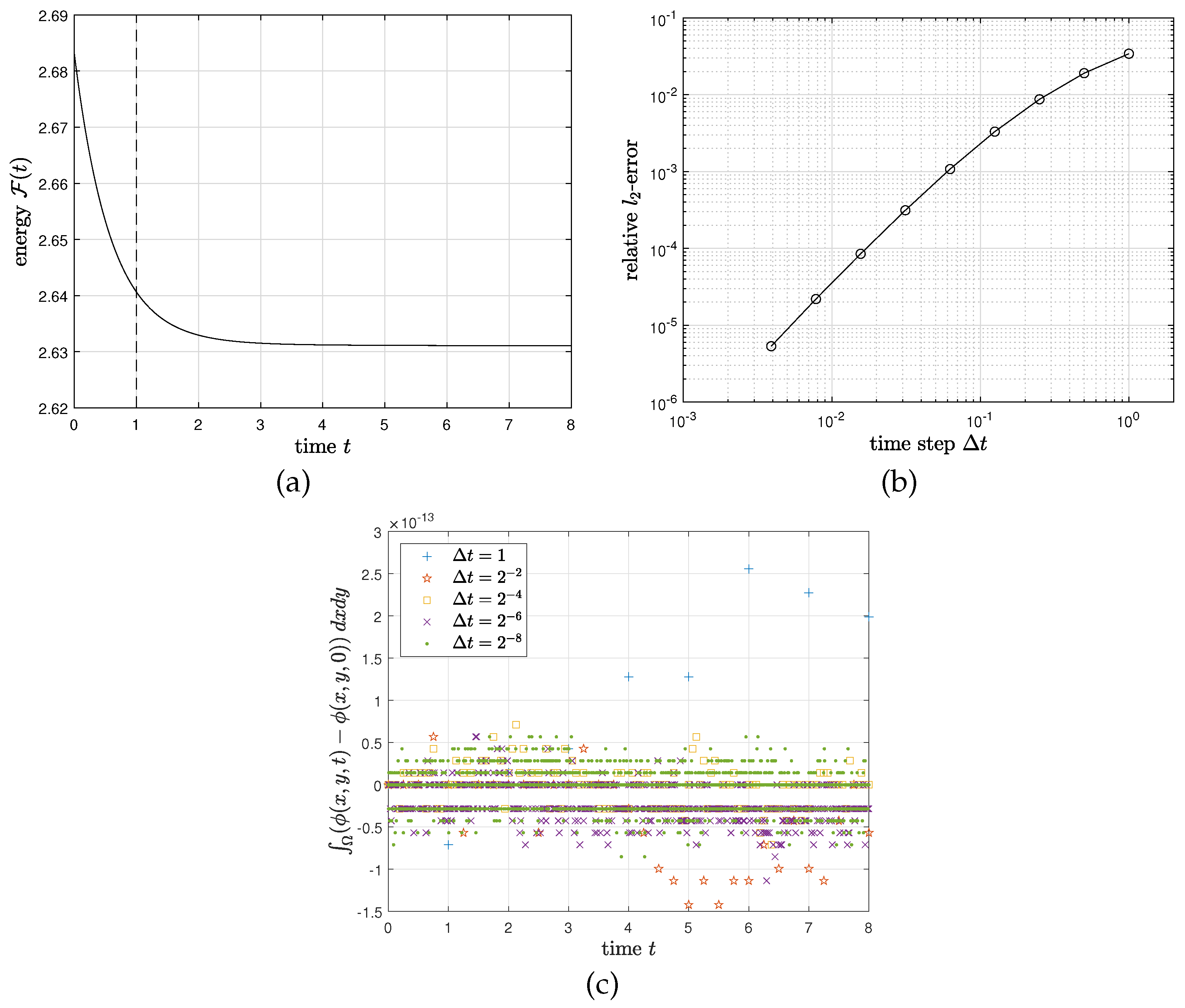
on $\Omega =[0,32]\times [0,32]$. We use $ϵ=0.025$, $A=1$, $B=3A^2$, and $\Delta x=\Delta y=\frac{1}{3}$. Figure 1a,b indicate the evolution of $\mathcal{F}\left(t\right)$ for the reference solution, with $\Delta t=2^{-10}$ and the relative $l_2$-errors of $\varphi (x,y,1)$ for various time steps, respectively. Here, the errors are calculated by comparison with the reference solution. Figure 1c also indicates the evolution of ${\int }_{\Omega }(\varphi (x,y,t)-\varphi (x,y,0))dxdy$. It is shown that the method is second-order convergent in time and conserves the mass.

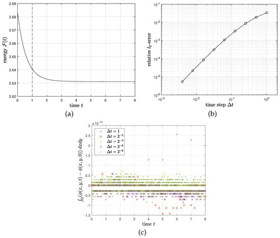
Figure 1. (a) Evolution of $\mathcal{F}\left(t\right)$ for the reference solution with $ϵ=0.025$, $\Delta x=\Delta y=\frac{1}{3}$, and $\Delta t=2^{-10}$. (b) Relative $l_2$-errors of $\varphi (x,y,1)$ for $\Delta t=2^{-8},2^{-7},\dots ,1$. (c) Evolution of ${\int }_{\Omega }(\varphi (x,y,t)-\varphi (x,y,0))dxdy$ for various time steps.

3.2. Energy Stability Test

To verify the energy stability of the proposed method, we take the initial condition (9) on $\Omega =[0,32]\times [0,32]$ and set $ϵ=0.25$, $A=1$, $B=3A^2$, and $\Delta x=\Delta y=\frac{1}{3}$. Figure 2a indicates the evolution of $\mathcal{F}\left(t\right)$ with several time steps. All energy curves non-increase over time, which demonstrates that the proposed method is unconditionally energy-stable (Theorem 2). Figure 2b indicates the evolution of $\varphi (x,y,t)$ with $\Delta t=2^{-4}$.

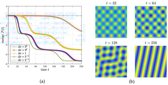
Figure 2. (a) Evolution of $\mathcal{F}\left(t\right)$ with several time steps. (b) Evolution of $\varphi (x,y,t)$ with $ϵ=0.25$, $\Delta x=\Delta y=\frac{1}{3}$, and $\Delta t=2^{-4}$. The yellow, green, and blue regions show $\varphi =0.6288$, $0.0688$, and $-0.4913$, respectively.

3.3. Pattern Formation

To compare the proposed method with other methods, we perform a long time simulation for pattern formation using the proposed method and the operator splitting method in [17]. An initial condition is:

$$\begin{array}{c}\hfill \varphi (x,y,0)=\overline{\varphi }+\mathrm{rand}(x,y)\end{array}$$

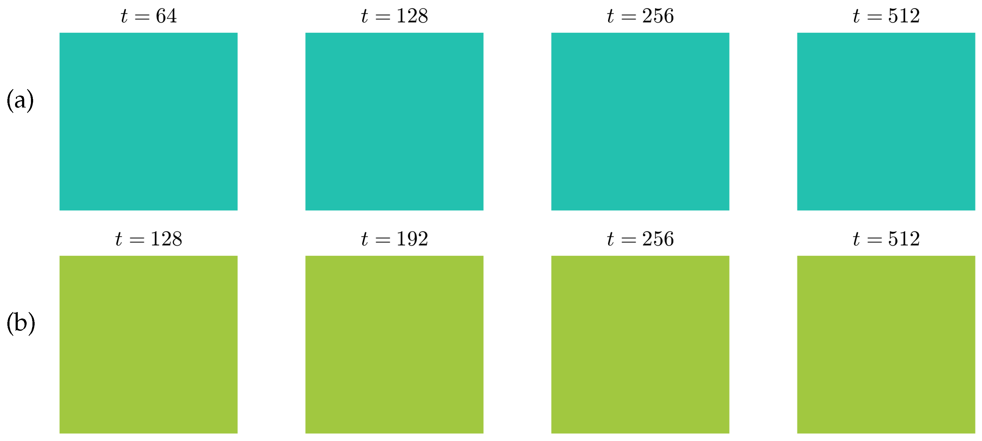
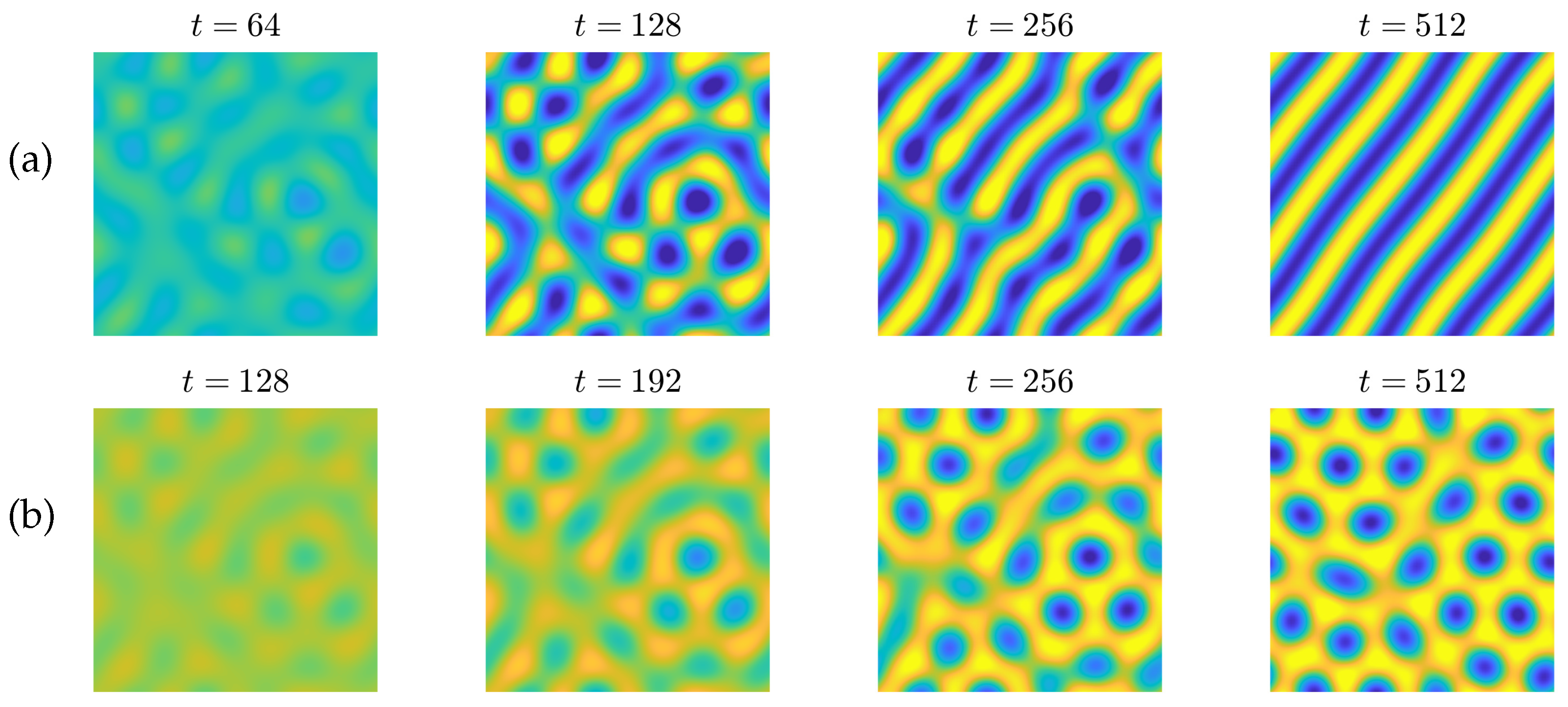
on $\Omega =[0,32]\times [0,32]$, where $\mathrm{rand}(x,y)$ is a random number between $-0.1$ and $0.1$ at the grid points. We choose $ϵ=0.2$, $A=1$, $B=3A^2$, $\Delta x=\Delta y=\frac{1}{3}$, and $\Delta t=2$. Figure 3a,b indicate evolutions of $\varphi (x,y,t)$ using the operator splitting method with $\overline{\varphi }=0.02$ and $0.2$, respectively. According to the phase diagram in [1], we expect striped and hexagonal states with $\overline{\varphi }=0.02$ and $0.2$, respectively. However, the operator splitting method with a large time step $\Delta t=2$ produces unexpected constant states. On the other hand, the proposed method leads to striped and hexagonal states even for $\Delta t=2$ (see Figure 4a,b).

Figure 3. Evolution of $\varphi (x,y,t)$ using the operator splitting method in [17] with (a) $\overline{\varphi }=0.02$ and (b) $0.2$. Here, $ϵ=0.2$, $\Delta x=\Delta y=\frac{1}{3}$, and $\Delta t=2$ are used. The yellow, green, and blue regions show $\varphi =0.5$, 0, and $-0.5$, respectively.

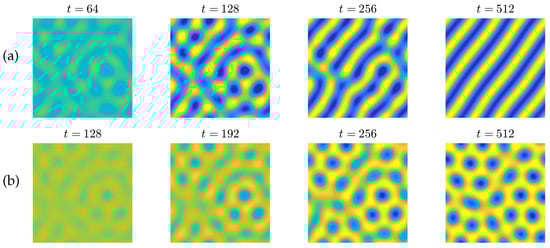
Figure 4. Evolution of $\varphi (x,y,t)$ using the proposed method with (a) $\overline{\varphi }=0.02$ and (b) $0.2$. Here, $ϵ=0.2$, $\Delta x=\Delta y=\frac{1}{3}$, and $\Delta t=2$ are used. The yellow, green, and blue regions show $\varphi =0.5$, 0, and $-0.5$, respectively.

3.4. Crystal Growth

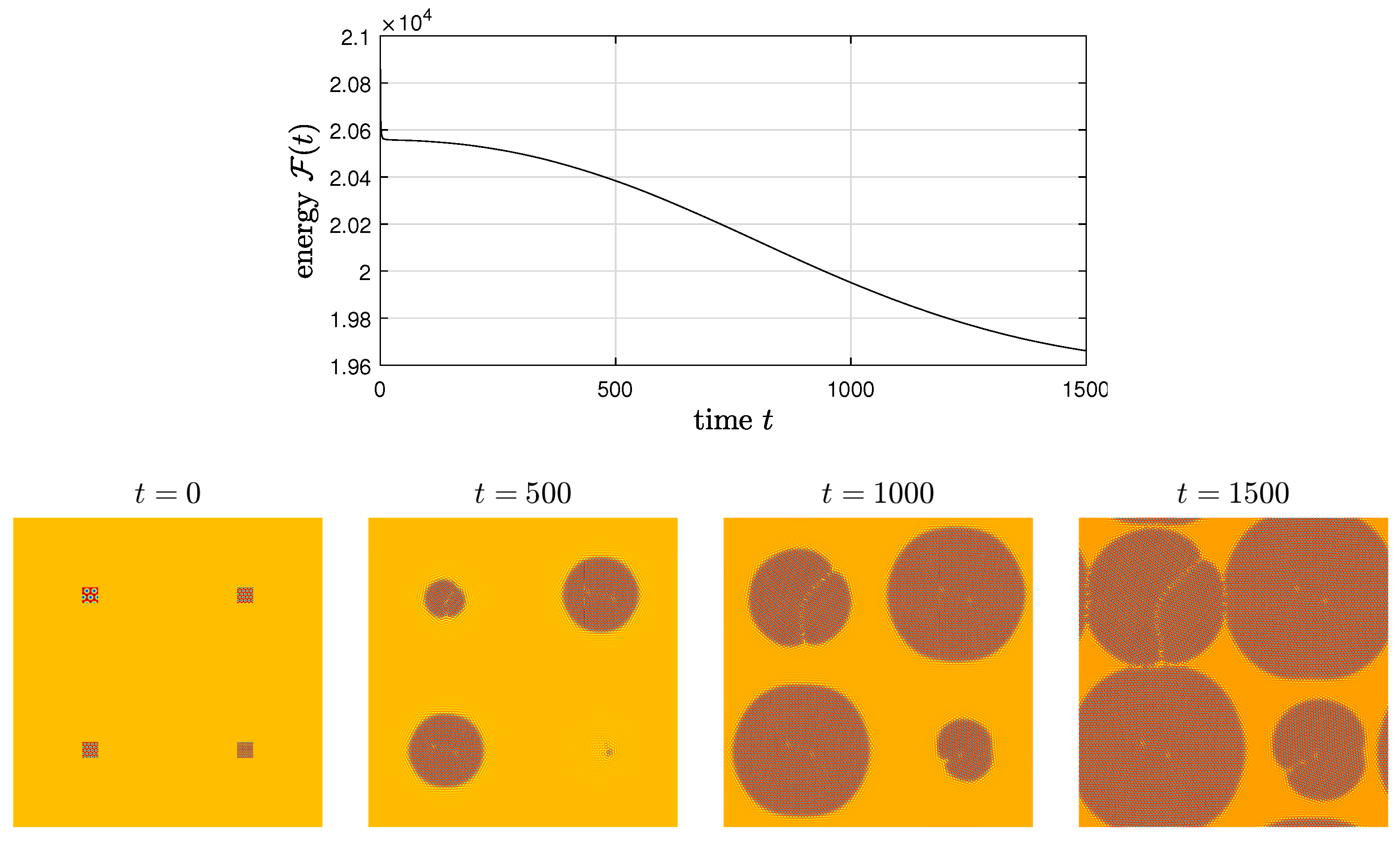
We simulate the growth and interaction of four crystallites on $\Omega =[0,512]\times [0,512]$ with $ϵ=0.25$, $A=1$, $B=3A^2$, $\Delta x=\Delta y=1$, and $\Delta t=1$. An initial condition is established by superposing the crystallites over a constant density field $\varphi (x,y,0)=\overline{\varphi }$. To define the crystallites, we employ the following expression:

$$\begin{array}{c}\hfill \varphi (x_l,y_l)=\overline{\varphi }+C\left(cos(\frac{q}{\sqrt{3}}{y}_l)cos(q{x}_l)-0.5cos(\frac{2q}{\sqrt{3}}{y}_l)\right),\end{array}$$

where $x_l$ and $y_l$ represent local Cartesian coordinates. For $\overline{\varphi }=0.285$, $C=0.45$, $q=0.5q_0,q_0,q_0,2q_0$ (from the top-left to the bottom-right), and $q_0=0.66$, Figure 5 indicates the evolution of $\mathcal{F}\left(t\right)$ and $\varphi (x,y,t)$. We can observe the energy dissipation and the interaction between growing crystallites.

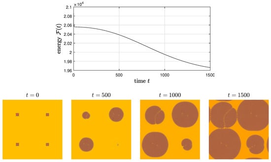
Figure 5. Evolution of $\mathcal{F}\left(t\right)$ and $\varphi (x,y,t)$ with $ϵ=0.25$, $\Delta x=\Delta y=1$, and $\Delta t=1$. The red, green, and blue regions show $\varphi =0.6475$, $0.0741$, and $-0.4993$, respectively.

4. Conclusions

To obtain numerical solutions for the $L^2$-PFC equation, we regularized $\frac{1}{4}{\varphi }^4$ in $\mathcal{F}\left(\varphi \right)$ by $f\left(\varphi \right)$ such that ${max}_{\varphi \in \mathbb{R}}\left|f^{″}\left(\varphi \right)\right|\le 3A^2$. Furthermore, we got the linear convex splitting by putting $f\left(\varphi \right)$ in ${\mathcal{F}}_e\left(\varphi \right)$, adding $\frac{B}{2}{\int }_{\Omega }{\varphi }^{2}d\mathbf{x}$ to ${\mathcal{F}}_e\left(\varphi \right)$, and setting $B\ge 3A^2$. Moreover, to preserve the mass conservation and energy stability, we applied the linear convex splitting to both $\nu$ and $\frac{1}{|\Omega |}{\int }_{\Omega }\nu d\mathbf{x}$. Finally, to achieve second-order time accuracy, we combined the second-order SSP-IMEX-RK method. Numerical experiments proved that the proposed method is second-order convergent in time, mass-conservative, and unconditionally energy-stable. By using the proposed method, we performed a long time simulation for pattern formation and crystal growth, where different patterns, depending on the value of $\overline{\varphi }$, and growing crystallites can be observed clearly.

References

- Elder, K.R.; Katakowski, M.; Haataja, M.; Grant, M. Modeling elasticity in crystal growth. Phys. Rev. Lett. 2002, 88, 245701. [Google Scholar] [CrossRef] [PubMed] [Green Version]
- Elder, K.R.; Grant, M. Modeling elastic and plastic deformations in nonequilibrium processing using phase field crystals. Phys. Rev. E 2004, 70, 051605. [Google Scholar] [CrossRef] [PubMed] [Green Version]
- Swift, J.; Hohenberg, P.C. Hydrodynamic fluctuations at the convective instability. Phys. Rev. A 1977, 15, 319–328. [Google Scholar] [CrossRef] [Green Version]
- Hu, Z.; Wise, S.M.; Wang, C.; Lowengrub, J.S. Stable and efficient finite-difference nonlinear-multigrid schemes for the phase field crystal equation. J. Comput. Phys. 2009, 228, 5323–5339. [Google Scholar] [CrossRef] [Green Version]
- Wise, S.M.; Wang, C.; Lowengrub, J.S. An energy-stable and convergent finite-difference scheme for the phase field crystal equation. SIAM J. Numer. Anal. 2009, 47, 2269–2288. [Google Scholar] [CrossRef] [Green Version]
- Gomez, H.; Nogueira, X. An unconditionally energy-stable method for the phase field crystal equation. Comput. Methods Appl. Mech. Engrg. 2012, 249–252, 52–61. [Google Scholar] [CrossRef]
- Vignal, P.; Dalcin, L.; Brown, D.L.; Collier, N.; Calo, V.M. An energy-stable convex splitting for the phase-field crystal equation. Comput. Struct. 2015, 158, 355–368. [Google Scholar] [CrossRef] [Green Version]
- Dehghan, M.; Mohammadi, V. The numerical simulation of the phase field crystal (PFC) and modified phase field crystal (MPFC) models via global and local meshless methods. Comput. Methods Appl. Mech. Engrg. 2016, 298, 453–484. [Google Scholar] [CrossRef]
- Shin, J.; Lee, H.G.; Lee, J.-Y. First and second order numerical methods based on a new convex splitting for phase-field crystal equation. J. Comput. Phys. 2016, 327, 519–542. [Google Scholar] [CrossRef]
- Yang, X.; Han, D. Linearly first-and second-order, unconditionally energy stable schemes for the phase field crystal model. J. Comput. Phys. 2017, 330, 1116–1134. [Google Scholar] [CrossRef] [Green Version]
- Li, X.; Shen, J. Stability and error estimates of the SAV Fourier-spectral method for the phase field crystal equation. Adv. Comput. Math. 2020, 46, 48. [Google Scholar] [CrossRef]
- Shin, J.; Lee, H.G.; Lee, J.-Y. Long-time simulation of the phase-field crystal equation using high-order energy-stable CSRK methods. Comput. Methods Appl. Mech. Eng. 2020, 364, 112981. [Google Scholar] [CrossRef]
- Zhang, J.; Yang, X. Efficient fully discrete finite-element numerical scheme with second-order temporal accuracy for the phase-field crystal model. Mathematics 2022, 10, 155. [Google Scholar] [CrossRef]
- Nawaz, R.; Ali, N.; Zada, L.; Shah, Z.; Tassaddiq, A.; Alreshidi, N.A. Comparative analysis of natural transform decomposition method and new iterative method for fractional foam drainage problem and fractional order modified regularized long-wave equation. Fractals 2020, 28, 2050124. [Google Scholar] [CrossRef]
- Farid, S.; Nawaz, R.; Shah, Z.; Islam, S.; Deebani, W. New iterative transform method for time and space fractional (n+1)-dimensional heat and wave type equations. Fractals 2021, 29, 2150056. [Google Scholar] [CrossRef]
- Zhang, J.; Yang, X. Numerical approximations for a new L2-gradient flow based Phase field crystal model with precise nonlocal mass conservation. Comput. Phys. Commun. 2019, 243, 51–67. [Google Scholar] [CrossRef]
- Lee, H.G. A new conservative Swift-Hohenberg equation and its mass conservative method. J. Comput. Appl. Math. 2020, 375, 112815. [Google Scholar] [CrossRef]
- Lee, H.G. Stability condition of the second-order SSP-IMEX-RK method for the Cahn–Hilliard equation. Mathematics 2020, 8, 11. [Google Scholar] [CrossRef] [Green Version]
- Chen, X.; Song, M.; Song, S. A fourth order energy dissipative scheme for a traffic flow model. Mathematics 2020, 8, 1238. [Google Scholar] [CrossRef]
- Shin, J.; Lee, H.G. A linear, high-order, and unconditionally energy stable scheme for the epitaxial thin film growth model without slope selection. Appl. Numer. Math. 2021, 163, 30–42. [Google Scholar] [CrossRef]
- Kim, J.; Lee, H.G. Unconditionally energy stable second-order numerical scheme for the Allen–Cahn equation with a high-order polynomial free energy. Adv. Differ. Equ. 2021, 2021, 416. [Google Scholar] [CrossRef]
- Lee, H.G. A non-iterative and unconditionally energy stable method for the Swift–Hohenberg equation with quadratic–cubic nonlinearity. Appl. Math. Lett. 2022, 123, 107579. [Google Scholar] [CrossRef]
- Lee, H.G.; Shin, J.; Lee, J.-Y. A high-order and unconditionally energy stable scheme for the conservative Allen–Cahn equation with a nonlocal Lagrange multiplier. J. Sci. Comput. 2022, 90, 51. [Google Scholar] [CrossRef]
Publisher’s Note: MDPI stays neutral with regard to jurisdictional claims in published maps and institutional affiliations. |
© 2022 by the author. Licensee MDPI, Basel, Switzerland. This article is an open access article distributed under the terms and conditions of the Creative Commons Attribution (CC BY) license (https://creativecommons.org/licenses/by/4.0/).