Article

Nonparametric Estimation of the Density Function of the Distribution of the Noise in CHARN Models

by
Joseph Ngatchou-Wandji
1,2,*,
Marwa Ltaifa
2,
Didier Alain Njamen Njomen
3 and
Jia Shen
4
1
EHESP French School of Public Health, 35043 Rennes, France
2
Institut Élie Cartan de Lorraine, University of Lorraine, 54052 Vandoeuvre-Lès-Nancy, France
3
Department of Mathematics and Computer Science, Faculty of Science, University of Maroua, Maroua P.O. Box 814, Cameroon
4
Department of Statistics, Fudan University, Shanghai 200433, China
*
Author to whom correspondence should be addressed.
Mathematics 2022, 10(4), 624; https://doi.org/10.3390/math10040624
Submission received: 31 December 2021 / Revised: 13 February 2022 / Accepted: 14 February 2022 / Published: 17 February 2022
(This article belongs to the Section Probability and Statistics)

Abstract

:
This work is concerned with multivariate conditional heteroscedastic autoregressive nonlinear (CHARN) models with an unknown conditional mean function, conditional variance matrix function and density function of the distribution of noise. We study the kernel estimator of the latter function when the former are either parametric or nonparametric. The consistency, bias and asymptotic normality of the estimator are investigated. Confidence bound curves are given. A simulation experiment is performed to evaluate the performance of the results.

1. Introduction

The importance of multivariate time series is highlighted in a number of papers. They are widely studied in the econometric and statistical literature as can be seen, for instance, in [1,2,3,4,5,6]. Because of the interesting features of conditional heteroscedastic models in the analysis of financial time series, a lot of work has been devoted to the study of ARCH models [7,8,9] which, motivated by many reasons, have been generalized to CHARN models [10]. The CHARN model we deal with here is described as follows:
X t = T ( Y t ) + V ( Y t ) ε t , t Z ,
where the sequence { X t = ( X t , 1 , , X t , k ) } is a stationary and ergodic k-dimensional process; the Y t = ( X t 1 , X t 2 , , X t p ) R p k are a p k -dimensional random vector; the ε t = ( ε t , 1 , , ε t , k ) , t Z are i.i.d. k-dimensional standard white noise with density function f; and ε t is uncorrelated with the σ -algebra spanned by the Y s ’s, s < t . The k-dimensional function T ( x ) = ( T 1 ( x ) , , T k ( x ) ) and the k × k positive definite matrix function V ( x ) = ( V i j ( x ) : 1 i , j k ) are either of unknown or known forms but depend on unknown parameters. Note that the T j ’s and V i , j ’s, 1 i , j k are real-valued functions defined on R p k .
It is well-known (see, for example, [6]) that an estimator of the noise distribution can be used for testing model assumptions. This is often used in time series analysis at the model validation step (see, for example, [11], Section 5.3, p. 164), where one checks whether the residuals from the model fit behave in a consistent manner with the model. In this sense, when the current model is fitted to observations, one should check if the residuals behave like observations from iid random vectors with a specified density f = f 0 . There are many existing tests, for the iid assumption (see, for example, [11]). If f 0 is the Gaussian density, one can use the Shapiro–Wilk test for testing the Gaussianity of the residuals. For a more general density, a simple test based on confidence bound functions for f can be used if these bounds can be constructed. Then, if the curve of the given f 0 lies between the bounds, one would accept that f = f 0 and that the residuals are from f 0 . Confidence bounds can be obtained if one constructs a consistent and asymptotic normal estimator of f. The present work focuses on the study of the kernel estimator of f based on the residuals. All along the paper, we assume that this function is positive, uniformly continuous and twice differentiable, with continuous and bounded derivatives.
If the ε t s are observed, the kernel estimator of f would be defined by
f n ( x ) = 1 n a n k t = 1 n K x ε t a n , x R k ,
where a n is the smoothing parameter and K a Parzen–Rosenblatt kernel ( | | x | | k K ( x ) 0 , | | x | | k ). Since these are never observed, they have to be substituted for estimates as, for example, residual series from parametric or nonparametric fits. In this paper, we study the asymptotic behavior of such an estimator. In Section 2, we write a short review on the kernel estimation of the density function. In Section 3, we study some asymptotic properties of f n ( x ) when the functions T and V are parametric and the ε t s are substituted for the residuals from the fit. In Section 4, the same is done when the latter functions are nonparametric. We do not study the asymptotic normality in this case, as it is too technical and lengthy. The results are illustrated by a simulation experiment in Section 5, and Section 6 contains our conclusion. In order to have a self-contained paper, the external results used along the current work are gathered in Appendix A.

2. On the Kernel Density Estimation

2.1. A Short Review

During the last four decades, nonparametric functional estimation has undergone considerable developments. In particular, the estimation of the density of a probability law in R k , k 1 , has been studied by very different methods, some of which include Refs. [12,13,14,15,16,17,18,19].
The first work in this field goes back to [20,21], which focused on the solution densities of a differential equation:
d g d x = ( x a ) g b 0 + b 1 x + b 2 x 2 ,
where the constants a , b 0 , b 1 and b 2 are expressed as functions of the first four moments of the distribution of the density g. For estimating g, the technique was to estimate the moments of this distribution.
Subsequently, many other methods have been proposed. Because of its ease, the kernel method received the most attention. This method was introduced by [22], from the idea of Fix and Hodges invoked in [23]. The idea consisted in estimating the density g at a point x by counting the number of observations located in the interval [ x a , x + a ] for a > 0 . Rosenblatt proposed a more general estimator defined by
g n ( x ) = 1 n a n i = 1 n K x U i a n , x R ,
where K is a probability density on R , ( a n ) is a sequence of positive real numbers, and U 1 , , U n is a sample from g. In the literature, g n is commonly referred to as the Parzen–Rosenblatt estimator [22,24]. Its extension to the multivariate case was studied by [25] who proposed as the estimator
g n ( x ) = 1 n a n k i = 1 n K x U i a n , x R k , k 1 ,
where K is a probability density on R k and the U i s are k-dimensional samples.
The scaling factor a n k appearing in the denominator in the right-hand side of (4) can be seen as the determinant of a k × k diagonal matrix with the a n s on the main diagonal. Moreover, the argument of the function K can also be seen as the transformation of x U i by the inverse of this matrix. From these observations [14], instead of considering a diagonal matrix, we rather considered a full matrix and defined the estimator
g ˜ n ( x ) = 1 n | det ( H n ) | i = 1 n K ( H n 1 ( x U i ) ) , x R k ,
where H n is an invertible k × k matrix with determinant det ( H n ) .
Ref. [26] introduced a new class of kernel estimators of the density of a probability distribution on R k , k 1 . The originality of these estimators compared to the previous ones is that the usual bandwidth a n is a function of the observations and its moments of orders 1 and 2 coincide with the empirical moments of the law to be estimated. However, this study was done for the normal kernel only.
For more on the kernel density estimation, the reader can refer to the monographs of [13,16,18,19,27,28]. A more recent book is that of [29], which also gathers numerous recent references on the subject.

2.2. Some Properties of the Kernel Estimator

The method which seems convenient, simple to implement, robust and does not require a multiple choice of parameters is the kernel method, which has attracted the most interest since [22,24]. The properties of the resulting kernel estimator g n have been largely studied in the literature.
Several modes of convergence of the kernel estimator g n to g have been studied. Ref. [24] for k = 1 and [25] for k > 1 , have established the convergence in probability. That is, as n , in probability,
sup x R k | g n ( x ) g ( x ) | 0 ,
and the convergence to 0 of the mean square error ( M S E )
M S E = E { [ g n ( x ) g ( x ) ] 2 } .
Ref. [30] obtained, for k = 1 , the convergence to 0 of the mean integrated squared error ( M I S E )
M I S E = R k E { [ g n ( x ) g ( x ) ] 2 } d x .
Ref. [18] stated and proved various results on the properties of the kernel estimator g n . Most of them are about its pointwise and uniform consistency, its asymptotic bias and variance, or its asymptotic normality. Those of these results used to establish our results are recalled in the last section.

2.3. Bandwidth Selection

Bandwidth selection is an important issue in the kernel estimation of density functions. It is crucial to the estimation accuracy. However, it is a difficult problem which has been the subject of a large amount of work (see, for example, [31] for a review). Unlike data-driven methods, such as least square or cross-validation selection (see, for example, [32]), the plug-in methods demonstrate their simplicity and adequacy in the symmetric density shape case. The following plug-in method is proposed by [14,33]. Resulted from the optimization of the M I S E above in certain cases, their bandwidth a n is taken to be
a n = K 2 ( t ) d t ( t 2 K ( t ) d t ) 2 1 / 5 S n ( 3 / 8 π ) 1 / 5 n 1 / 5 ,
where S n 2 = n 1 i = 1 n ( U i U ¯ ) 2 is the sample variance. With the Epanechnikov kernel, this bandwidth is approximately defined as
a n = 1.0486 S n n 1 / 5 .
It is this bandwidth that is further used in the numerical study in Section 5 of this paper.

3. The Semi-Parametric Models Case

Here, we consider model (1) with the aim of estimating f by a kernel method in the case T ( x ) = M ( θ ; x ) and V ( x ) = Σ ( θ ; x ) for some k-dimensional vector M and k × k matrix Σ functions of known forms, with the unknown parameter θ = ( θ 1 , , θ q ) lying within a subset Θ of R q . More precisely, we study some of the asymptotic properties of f n ( x ) defined by (2) when the ε t s are substituted for the residuals from the fit. This requires the estimation of the parameter vector θ . In the following subsection, we briefly review some recent results on this estimation.

3.1. The Parameter Estimation

There is an increasing body of work on the parameter estimation of many classes of models contained within CHARN models (1). In this subsection, we give an overview of some of them.
The main estimators encountered in the time series literature are of least squares (LS) or of the likelihood type. Besides these, are some other less popular ones. Ref. [34] constructed a Godambe’s estimator, which they denoted by G, and proved that it is more efficient than the conditional least-squares estimator (CL) for autoregressive conditional heteroscedasticity (ARCH) models. In [35], the efficiency of the CL- and G-estimators for the CHARN model was studied. Ref. [35] deduced the condition according to which the estimator G is asymptotically optimal. The author proved the asymptotic normality of these two estimators and concluded that the G-estimator is less efficient than the CL-estimator.
The aim of [36] was to study the estimation function theory proposed by [37,38,39] for CHARN models. More precisely, Ref. [36] proposed a general estimator of the estimation function and derived its asymptotic distribution.
Ref. [40] introduced a method for the parameters estimation of ARCH models. They derived the optimal estimating function (EF) by combining linear and quadratic estimating functions. They proved that this estimator is more efficient than the quasi-maximum-likelihood estimator and, under the conditional normality assumption, the constructed EF-estimator is identical to that obtained by using the maximum-likelihood method in finite samples. The simulation results show that the finite-sample properties of the EF-estimators are attractive. The latter tends to display less bias and root mean squared error than the quasi-maximum likelihood estimator.
Ref. [41] studied parameter estimation in a class of CHARN models. He investigated the properties of the conditional least-squares estimators and those of the conditional likelihood estimators. He defined the kernel estimators of noise density and its derivatives, and showed that they are uniformly consistent.
Several papers discussed the problem of estimation and inference in the exponential autoregressive models (EXPAR) introduced by [42]. Among others, one can cite [43,44,45,46,47,48].

3.2. The Kernel Estimation of the Density Function of the Noise

Denote by | | U | | an appropriate norm of a vector or a matrix U, and by U θ ( θ ; z ) the matrix of the partial derivatives with respect to θ , of the entries of a vector or matrix function U ( θ ; z ) . In the sequel, we restrict ourselves to identifiable models (1) for which the following hold:
(A1) 
For all θ Θ R q and z R p k , Σ ( θ ; z ) is invertible with inverse Σ 1 ( θ ; z ) .
(A2) 
The functions θ M ( θ ; z ) , θ Σ ( θ ; z ) and θ Σ 1 ( θ ; z ) are each continuously differentiable with respect to θ int ( Θ ) . There exists a finite positive number r such that the closed ball B ¯ ( θ 0 , r ) is contained within int ( Θ ) , and a positive function γ ( z ) with E γ 2 + β ( Y 0 ) < such that
max sup θ B ¯ ( θ 0 , r ) M θ ( θ ; z ) , sup θ B ¯ ( θ 0 , r ) Σ θ ( θ ; z ) , sup θ B ¯ ( θ 0 , r ) Σ 1 θ ( θ ; z ) γ ( z ) .
(A3) 
The true parameter θ 0 Θ has a consistent estimator θ ˜ n = ( θ ˜ n , 1 , , θ ˜ n , q ) satisfying
E [ | | n ( θ ˜ n θ 0 ) | | 2 ] ρ < , n
and
n ( θ ˜ n θ 0 ) N ( 0 , Δ ) ,
where “⟹” denotes the convergence in distribution, and Δ is a q × q positive definite matrix.
Remark 1.
Assumptions (A1)–(A2) hold at least for some usual stationary multivariate time series models, such as vector ARMA, vector EXPAR or vector ARCH models. Assumption (A3) holds for the estimators θ ˜ n satisfying the so-called Bahadur representation, as the likelihood, pseudo-likelihood, least-squares, conditional likelihood or conditional least-square estimators.
From model (1), by (A1), define for any t Z , and for any θ Θ ,
ε t ( θ ) = Σ 1 ( θ ; Y t ) X t M ( θ ; Y t ) , θ Θ , a n d ε ˜ t = ε t ( θ ˜ n ) .
Proposition 1.
Assume that assumptions (A1)–(A3) hold. Then, for any t Z ,
ε t ˜ P ε t ( θ 0 ) , n .
Proof. 
For any t Z , one can write
ε ˜ t ε t ( θ 0 ) = ε t ( θ ˜ n ) ε t ( θ 0 ) = Σ 1 ( θ ˜ n ; Y t ) X t M ( θ ˜ n ; Y t ) Σ 1 ( θ 0 ; Y t ) X t M ( θ 0 ; Y t ) = Σ 1 ( θ ˜ n ; Y t ) M ( θ 0 ; Y t ) M ( θ ˜ n ; Y t ) Σ 1 ( θ 0 ; Y t ) Σ 1 ( θ ˜ n ; Y t ) X t M ( θ 0 ; Y t ) = Σ 1 ( θ ˜ n ; Y t ) M ( θ 0 ; Y t ) M ( θ ˜ n ; Y t ) Σ 1 ( θ 0 ; Y t ) Σ 1 ( θ ˜ n ; Y t ) Σ ( θ 0 ; Y t ) ε t ( θ 0 ) .
Applying a first-order Taylor expansion to the differences within the above couples of brackets, since θ ˜ n is consistent to θ 0 , the desired result follows immediately by assumptions (A2) and (A3).
Let K ˜ be an almost-everywhere-differentiable Parzen–Rosenblatt kernel with gradient function K ˜ x ( x ) at x. One considers the kernel estimator of f defined by
f ˜ n ( x ) = 1 n a n k t = 1 n K ˜ x ε ˜ t a n , x R k ,
where the kernel function K ˜ and the bandwidth a n satisfy the following assumptions:
(A4) 
K ˜ is positive, even, and has compact support and bounded variation.
(A5) 
a n 0 , n a n k , n .
(A6) 
For all 0 and x , y R k , a n y K ˜ x ( x a n 1 ) 0 , as n , and y y 0 , and the sequence of functions a n K ˜ x ( x a n 1 ) is bounded.
Remark 2.
It can be easily verified that assumptions (A4) and (A6) hold at least for Gaussian and Epanechnikov kernels. As a consequence of (A4), | | y | | 2 K ˜ ( y ) d y < . Assumption (A5) implies that n a n k / log ( n ) as n .

3.2.1. The Consistency of f ˜ n to f

Proposition 2.
Assume that the assumptions (A1)–(A6) are satisfied. Then,
sup x R k | f ˜ n ( x ) f ( x ) | = o P ( 1 ) .
Proof. 
For any t Z , recall the form of the k × q matrix ε t θ :
ε t θ = ε t , 1 θ ε t , k θ ,
where for any, t Z , 1 j k ,
ε t , j θ = ε t , j θ 1 , , ε t , j θ q .
For any x R k ,
f ˜ n ( x ) f n ( x ) = 1 n a n k t = 1 n K ˜ x ε ˜ t a n K ˜ x ε t a n 1 n a n k t = 1 n K ˜ x ε ˜ t a n K ˜ x ε t a n 1 n t = 1 n 1 a n k + 1 ( ε ˜ t ε t ) K ˜ x x ε . t a n ,
where ε . t lies between ε ˜ t and ε t .
Since for t Z , ε ˜ t tends in probability to ε t as n tends to infinity, in view of our assumptions, one has that, in probability,
1 a n k + 1 ( ε ˜ t ε t ) K ˜ x x ε . t a n 0 as n .
By a stochastic version of the Cesàro theorem (see Appendix A), one has that, in probability, the right-hand side of the last inequality tends to 0 as n tends to infinity. Consequently, in probability,
sup x R k f ˜ n ( x ) f n ( x ) 0 , n .
Now, by Theorem 1 in Appendix A.1, it follows that, in probability,
sup x R k f n ( x ) f ( x ) 0 as n .
Whence, in probability,
sup x R k f ˜ n ( x ) f ( x ) 0 as n .

3.2.2. The Bias Study

Proposition 3.
Assume that assumptions (A1)–(A6) hold. Then,
x R k , E [ f ˜ n ( x ) ] f ( x ) 0 , n .
Proof. 
For all x = ( x 1 , , x k ) R k , define the function
χ k ( x ) = 1 i , j k 2 f x i x j ( x ) t i t j K ( t 1 , , t k ) d t 1 d t k .
Then for all x = ( x 1 , , x k ) R k ,
E [ f ˜ n ( x ) ] f ( x ) = E [ f ˜ n ( x ) f n ( x ) ] + [ E ( f n ( x ) ) f ( x ) ] = 1 n a n k t = 1 n E [ K ˜ x ε ˜ t a n K ˜ x ε t a n ] + a n 2 2 χ k ( x ) + o ( a n 2 ) .
For all t Z and x R k , define the functions
d t ( x ) = 1 a n k E K ˜ x ε ˜ t a n K ˜ x ε t a n w n ( x ) = 1 n t = 1 n d t ( x ) .
With these, one can write, for all x R k ,
E [ f ˜ n ( x ) ] f ( x ) = w n ( x ) + a n 2 2 χ k ( x ) + o ( a n 2 ) .
Now, we show that for all x R k , in probability, w n ( x ) 0 as n tends to .
By a first-order Taylor expansion of the function K ˜ , one obtains for all x R k and t Z ,
K ˜ x ε ˜ t a n K ˜ x ε t a n = 1 a n ( ε ˜ t ε t ) K ˜ x x ε t . a n ,
where for all t Z , ε t . lies between ε t and ε ˜ t .
By another first-order Taylor expansion applied to ε t = ε t ( θ ) , one then obtains, for some θ ˙ n = ( θ ˙ 1 n , , θ ˙ q n ) lying between θ ˜ n and θ ,
K ˜ x ε ˜ t a n K ˜ x ε t a n = 1 a n ε t θ ( θ ˙ n ) ( θ ˜ n θ ) K ˜ x x ε t . a n
It results that, for all t Z and x R k ,
d t ( x ) = 1 n a n k E 1 a n ε t θ ( θ ˙ n ) n ( θ ˜ n θ ) K ˜ x x ε t . a n .
By the Cauchy–Schwarz inequality, one has for all t Z and x R k ,
| d t ( x ) | 1 n a n k E 1 / 2 ε t θ ( θ ˙ n ) 1 a n K ˜ x x ε t . a n 2 E 1 / 2 | | n ( θ ˜ θ ) | | 2 .
By our assumptions and the dominated convergence theorem, it is easy to see that for all t Z , x R k ,
d t ( x ) 0 , n .
Whence, by Cesàro’s theorem (see Appendix A), one has that for all x R k ,
w n ( x ) = 1 n t = 1 n d t ( x ) 0 , n .
Given that for all x R k , a n 2 2 χ k ( x ) + o ( a n 2 ) tends to 0 as n tends to , one can then conclude that for all x R k ,
E [ f ˜ n ( x ) ] f ( x ) = w n ( x ) + a n 2 2 χ k ( x ) + o ( a n 2 ) 0 , n .
This shows that for all x R k , f ˜ n ( x ) is an asymptotically unbiased estimator of f ( x ) . □

3.2.3. Asymptotic Normality

Proposition 4.
Assume that (A1)–(A6) hold. Then
x R k , n a n k f ˜ n ( x ) f ( x ) ( f ( x ) K ˜ 2 ( u ) d u ) 1 / 2 N ( 0 , 1 ) .
Proof. 
One has for all x R k ,
n a n k [ f ˜ n ( x ) f ( x ) ] = n a n k [ f ˜ n ( x ) f n ( x ) ] + n a n k [ f n ( x ) f ( x ) ] .
We first study the first term in the right-hand side of the above equality.
For all x = ( x 1 , , x k ) R k , by applications of Taylor expansions to K ˜ and ε t respectively, one can write
n a n k [ f ˜ n ( x ) f n ( x ) ] = 1 n a n k t = 1 n K ˜ x ε ˜ t a n K ˜ x ε t a n = 1 n a n k t = 1 n 1 a n ( ε t ε ˜ t ) K ˜ x x ε . t a n . = 1 n a n k t = 1 n 1 a n ε t θ ( θ ˙ n ) ( θ ˜ θ ) K ˜ x x ε . t a n . = 1 n t = 1 n 1 a n 1 + k 2 ε t θ ( θ ˙ n ) n ( θ ˜ θ ) K ˜ x x ε . t a n ,
where ε . t lies between ε t and ε ˜ t , and θ ˙ n lies between θ ˜ n and θ .
Define for all t Z and all x R k ,
l t ( x ) = 1 a n 1 + k ε t θ ( θ ˙ n ) K ˜ x x ε . t a n .
By our assumptions, for any x R k , l t ( x ) tends in probability to 0 as n tends to infinity. Now, it is easy to see that
n a n k [ f ˜ n ( x ) f n ( x ) ] 1 n t = 1 n l t ( x ) | | n ( θ ˜ n θ ) | | a n .
By assumption (A3), | | n ( θ ˜ n θ ) | | is tight. Thus, for all t Z and all x R k , l t ( x ) | | n ( θ ˜ n θ ) | | a n tends in probability to 0 as n tends to infinity. By a stochastic version of the Cesàro theorem (see Appendix A.4), for all x R k , in probability,
n a n k [ f ˜ n ( x ) f n ( x ) ] 0 , n .
Since from Theorem A3 in Appendix A.3, one has that for all x R k ,
n a n k f n ( x ) f ( x ) N 0 , f ( x ) K ˜ 2 ( u ) d u ,
it results that for all x R k , as n tends to infinity,
n a n k [ f ˜ n ( x ) f ( x ) ] N 0 , f ( x ) K ˜ 2 ( u ) d u .
Then one concludes that for all x R k , as n tends to infinity,
n a n k f ˜ n ( x ) f ( x ) ( f ( x ) K ˜ 2 ( u ) d u ) 1 / 2 N ( 0 , 1 ) .
Proposition 5.
Assume that assumptions (A1)–(A6) hold. Then,
n a n k f ˜ n ( t i ) f ( t i ) f ( t i ) K ˜ 2 ( u ) d u 1 2 , 1 i N N ( 0 , I ) ,
where N ( 0 , I ) denotes the standard ℓ-dimensional Gaussian random vector, N , t i R k , 1 i k .
Proof. 
For all N , one can write
n a n k f ˜ n ( t i ) f ( t i ) f ( t i ) K ˜ 2 ( u ) d u 1 2 , 1 i = n a n k f ˜ n ( t i ) f n ( t i ) f ( t i ) K ˜ 2 ( u ) d u 1 2 , 1 i + n a n k f n ( t i ) f ( t i ) f ( t i ) K ˜ 2 ( u ) d u 1 2 , 1 i .
From Theorem A3 in Appendix A.3, as n , one has that
n a n k f n ( t i ) f ( t i ) f ( t i ) K ˜ 2 ( u ) d u 1 2 , 1 i N .
It follows from the proof of the above Proposition 4 that for t R k , fixed,
n a n k f ˜ n ( t ) f n ( t ) f ( t ) K ˜ 2 ( u ) d u 1 2 0 ,   n .
It results from the above that as n , one has that
n a n k f ˜ n ( t i ) f n ( t i ) f ( t i ) K ˜ 2 ( u ) d u 1 2 , 1 i ( 0 , , 0 ) .
So, as n , one has
n a n k f ˜ n ( t i ) f ( t i ) f ( t i ) K ˜ 2 ( u ) d u 1 2 , 1 i N .
A direct consequence of the above proposition is given by the following result. □
Proposition 6.
Assume that assumptions (A1)–(A6) hold. Then, for all x R k , a confidence band for f ( x ) at risk α [ 0 , 1 ] is given by
C B α ( x ) = f ˜ n ( x ) q 1 α 2 ( f ˜ n ( x ) K ˜ 2 ( u ) d u ) 1 / 2 n a n k ; f ˜ n ( x ) + q 1 α 2 ( f ˜ n ( x ) K ˜ 2 ( u ) d u ) 1 / 2 n a n k ,
where q 1 α 2 stands for the ( 1 α 2 ) -quantile of the standard Gaussian distribution.

4. The Nonparametric Models Case

Here, considering model (1), we estimate f by a kernel method in the case that the vector and matrix functions T and V ( x ) are unknown with unknown forms. That is, they are nonparametric functions. Because the study is lengthy and too technical, unlike in the preceding section, we only study the consistency and the bias of f n ( x ) defined by (2) when the ε t s are substituted for the residuals from the fit. In the first subsection, we give a brief review of some recent results on nonparametric estimation of T and V. The consistency and the bias studies are performed in the second subsection.

4.1. The Conditional Mean and Variance Functions Estimation

In the literature, the conditional mean (autoregression function) and the conditional variance (volatility) are estimated in various nonparametric methods. The estimators of the autoregression function are generally constructed and studied in the same ways as those of the well-known regression function. The pointwise convergence of this function was studied by [49,50,51]. The uniform convergence due to [52] generalizes the earlier results of [53,54,55,56]. The speed of convergence was treated by [57,58]. The L p convergence was obtained by [59,60,61,62], Gyorfi (1981). The assessment of bias and asymptotic variance were obtained by [49] for k = 1 and [63,64] for k 1 .
Ref. [65] considered model (1) in which both T and V are unknown functions of the past. Nonparametric estimators of these functions are constructed based on local polynomial fitting. They examined the rate of convergence of these estimators and established their asymptotic normality. Indeed, they generalized the result of [9] to a wider class of conditional mean and variance functions that can be seen as a limit of CHARN models, which themselves are generalizations of the ARCH structure.
Ref. [66] studied kernel methods based on weighted averages of response variables. The resulting estimators are very sensitive to large fluctuations in the data. To overcome this drawback, Ref. [67] used a robust estimation. This allowed the authors to extend the results of [66] to a large class of processes under stationarity and ergodicity. They proposed a family of robust nonparametric estimators of the regression or autoregression functions based on the kernel method. They subsequently established the uniform convergence of this family of estimators in the case that the observations are not bounded and belong to an increasing series of compacts. Ref. [68] considered model (1). They proposed an efficient and adaptive method for estimating the conditional variance. Their basic idea is to apply local linear regression to the squared residuals. They proved that, without knowing the regression function, they can estimate the conditional variance asymptotically as well as if the regression were given. Ref. [69] surveyed the semi-parametric and nonparametric methods in univariate and multivariate ARCH/GARCH models. They introduced some specific semi-parametric models and investigated the semi-parametric and nonparametric estimation techniques applied to the error density, the functional form of the volatility functions, the relationships between mean and variance, long memory processes, locally stationary processes, continuous time processes and multivariate models. Ref. [70] applied bootstrap methods to CHARN models and gave non-parametric estimators of the trend and volatility function. Ref. [71] studied the estimation of regression and volatility functions of nonlinear autoregressive models with ARCH errors. In [72], the nonparametric local exponential estimator was applied to estimate conditional volatility functions, ensuring its non-negativity. It is proved there that the obtained estimator is asymptotically fully adaptive to unknown conditional mean functions. Ref. [73] proposed a kernel weighted version of the standard realized integrated volatility estimator and gave sample properties. In addition, Ref. [74] constructed a spot volatility estimator for high-frequency financial data which contain market microstructure noise, proved the consistency of this estimator and derived its asymptotic distribution. The aim of [75] was to establish asymptotic results for estimators of functions and functionals linked to various models. The studied estimators are built on the basis of nonparametric methods. Ref. [76] considered a multidimensional nonparametric additive regression model with dependent observations. the authors used the marginal integration technique and wavelets methodology to develop a new adaptive estimator for a component of the additive regression function. Refs. [67,77,78] proposed a family of robust nonparametric estimators for regression or autoregression functions in a univariate or multivariate context.

4.2. The Kernel Estimation of the Density of the Noise

In this subsection, we assume the functions T and V unknown and nonparametric with unknown forms. We study the kernel estimator defined by (2) when the ε t s are substituted for the residuals from the fit. For the reasons mentioned in the introduction, we do not study the asymptotic normality of this estimator.
Let T ^ = ( T ^ 1 , , T ^ k ) , V ^ = ( V ^ i j ) and V ^ 1 = ( V ^ i j 1 ) be nonparametric estimators of T = ( T 1 , , T k ) , V = ( V i j ) and V 1 = ( V i j 1 ) , respectively, satisfying, for any t Z ,
(A7) 
T ^ ( Y t ) T ( Y t ) = o P ( 1 ) , V ^ ( Y t ) V ( Y t ) = o P ( 1 ) , V ^ 1 ( Y t ) V 1 ( Y t ) = o P ( 1 ) .
Remark 3.
(A7) is readily satisfied by estimators derived in some of the references cited above. T ^ can be obtained by kernel methods as in [66,67] or by local polynomial methods as in [6], or by adaptive methods as in [76]. V ^ can be obtained by local polynomial approaches as in [1,6,65] or by a local exponential method as in [72].
For any t Z , define
ε t = ε t ( T , V ) = V 1 ( Y t ) X t T ( Y t ) a n d ε ^ t = ε t ( T ^ , V ^ ) .
It is easy to see from assumption (A7) that for any t Z ,
ε ^ t = ε t + o P ( 1 ) .
In the sequel, the kernel considered is denoted by K ^ rather than K ˜ as in the preceding section. We study the asymptotic behavior of the following kernel estimator:
f ^ n ( x ) = 1 n a n k t = 1 n K ^ x ε ^ t a n , x R k .
Proposition 7.
Assume that (A4)–(A7) hold. Then, in probability,
sup x R k f ^ n ( x ) f ( x ) 0 , n .
Proof. 
For all x = ( x 1 , , x k ) R k , one can write
f n ^ ( x ) f n ( x ) = 1 n a n k t = 1 n K ^ x ε ^ t a n K ^ x ε t a n = | 1 n a n k t = 1 n [ K ^ x V ^ 1 ( Y t ) X t T ^ ( Y t ) a n K ^ x V 1 ( Y t ) X t T ( Y t ) a n ] | 1 n a n k t = 1 n | K ^ x V ^ 1 ( Y t ) X t T ^ ( Y t ) a n K ^ x V 1 ( Y t ) X t T ( Y t ) a n | .
Recalling that K x ( x ) denotes the transpose of K x ( x ) , by a Taylor expansion of K ^ , one has
K ^ x V ^ 1 ( Y t ) X t T ^ ( Y t ) a n K ^ x V 1 ( Y t ) X t T ( Y t ) a n = 1 a n K ^ x ε . t , x a n V 1 ( Y t ) X t T ( Y t ) V ^ 1 ( Y t ) X t T ^ ( Y t ) ,
where for any t Z , x R k , ε . t , x is a random vector lying between x ε t and x ε ^ t .
Now, observing that
V 1 ( Y t ) X t T ( Y t ) V ^ 1 ( Y t ) X t T ^ ( Y t ) = V 1 ( Y t ) V ^ 1 ( Y t ) ε t ( T , V ) + V ^ 1 ( Y t ) T ^ ( Y t ) T ( Y t )
It results from this that
sup x R k f ^ n ( x ) f n ( x ) 1 n t = 1 n sup x R k | 1 a n k + 1 K ^ x ε . t , x a n V 1 ( Y t ) V ^ 1 ( Y t ) ε t ( T , V ) + V ^ 1 ( Y t ) T ^ ( Y t ) T ( Y t ) | .
By our assumptions, the terms in the summand in the right-hand side of the above inequality tends to 0 as n tends to infinity. Then, by a stochastic version of the Cesàro theorem (see Appendix A.4), in probability,
sup x R k f ^ n ( x ) f n ( x ) 0 , n .
It is well known (see Theorem A1, Appendix A.1) that, in probability,
sup x R k | f n ( x ) f ( x ) | 0 , n .
Consequently, in probability,
sup x R k f ^ n ( x ) f ( x ) 0 , n .

Bias Study of f ^ n

Proposition 8.
Assume that (A4)–(A7) hold, and that K ^ is bounded by a positive number. Assume that | | x | | f ( x ) d x < . Then, for all x R k , f ^ n ( x ) is an asymptotically unbiased estimator of f ( x ) .
Proof. 
For all x R k ,
E [ f ^ n ( x ) ] f ( x ) = E [ f ^ ( x ) f n ( x ) ] + E [ f n ( x ) ] f ( x ) .
By Theorem A2 in Appendix A.2, as n ,
E f n ( x ) f ( x ) 0 .
Now, we show that for all x R k , as n ,
E [ f ^ n ( x ) f n ( x ) ] 0 .
Indeed, for x R k ,
E [ f ^ n ( x ) f n ( x ) ] = 1 n a n k t = 1 n E K ^ x ε ^ t a n K ^ x ε t a n = 1 n t = 1 n E 1 a n k + 1 ( ε ^ t ε t ) K ^ x x ε . t a n = 1 n t = 1 n L t ( x ) ,
where, for any t Z and x R k ,
L t ( x ) = E 1 a n k + 1 ( ε ^ t ε t ) K ^ x x ε . t a n = E { 1 a n k + 1 K ^ x x ε . t a n V 1 ( Y t ) V ^ 1 ( Y t ) ε t ( T , V ) + V ^ 1 ( Y t ) T ^ ( Y t ) T ( Y t ) } ,
where for all t Z , ε t . lies between ε ^ t and ε t .
Since for all t Z , T ( Y t ) T ^ ( Y t ) and V 1 ( Y t ) V ^ 1 ( Y t ) 0 in probability as n . The above terms in the pairs of brackets tend to 0 in probability as n tends to infinity. It follows from our assumptions that for all t Z and all x R k ,
L t ( x ) 0 , n .
Thus, by the Cesàro Theorem, for all x R k ,
E [ f ^ n ( x ) f n ( x ) ] = 1 n t = 1 n L t ( x ) 0 , n .
This concludes the proof of the result. □

5. Simulation Experiments

In this section, we conduct a simulation experiment to evaluate the finite sample properties of the estimators studied in the preceding sections. We restrict to the cases k = 1 , 2 . For k = 1 , we study the situation where the conditional mean and variance functions are parametric, and where they are nonparametric. For k = 2 , we only study the case that these functions are parametric.
Although we do not study the asymptotic normality of the kernel estimator in the case that the functions T and V are nonparametric, we construct heuristically asymptotic confidence-bound functions in the lines of those obtained in the case that T and V are parametric.

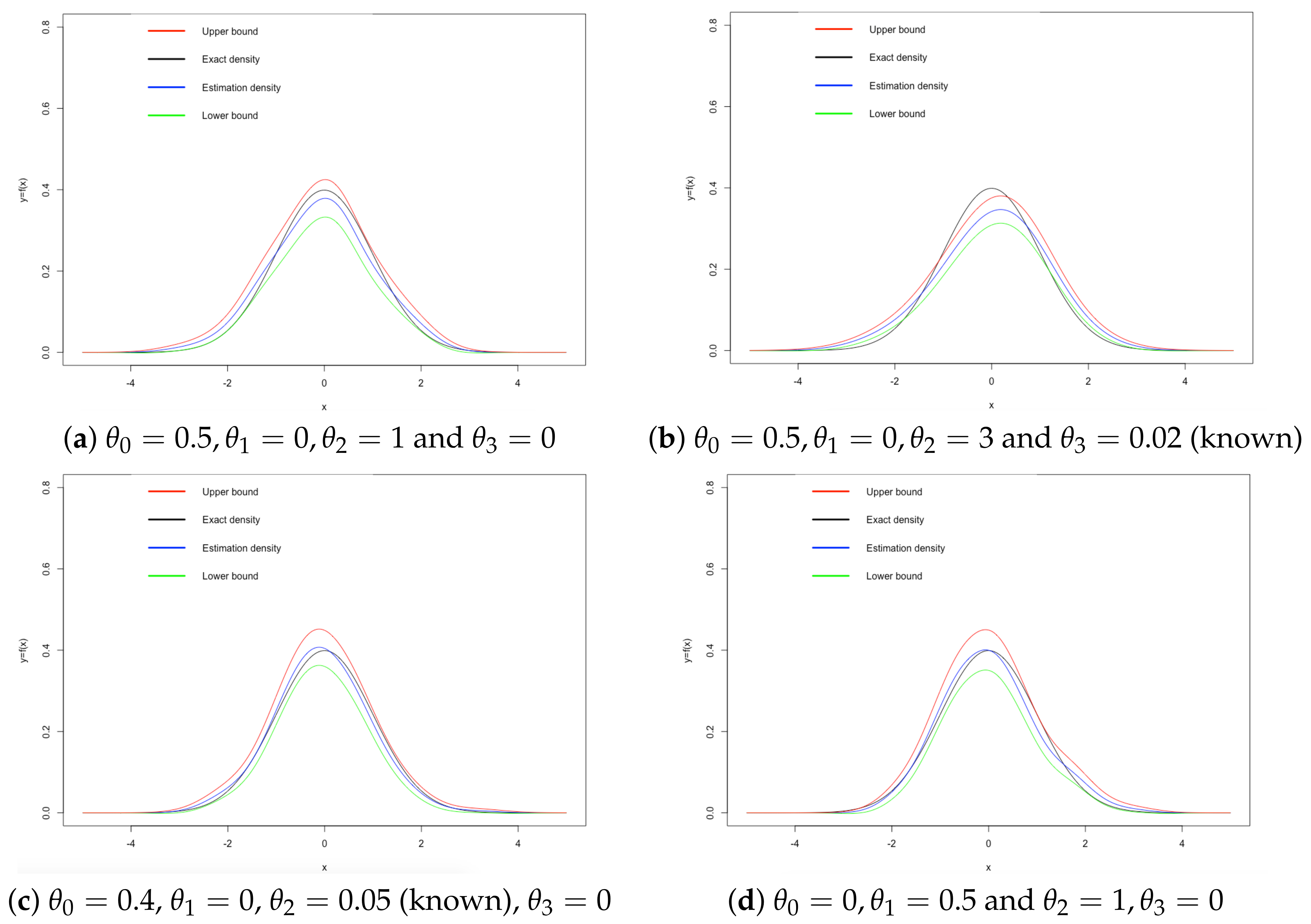
5.1. Unidimensional Case

Let θ = ( θ 0 , θ 1 , θ 2 , θ 3 ) . For several values of θ , we generate n observations from model (1) with
T ( x ) = θ 0 + θ 1 e 0.03 x 2 x and V ( x ) = θ 2 + θ 3 x 2
and f is the standard Gaussian density function. Once the data are generated, in order to apply our results, we first assume that functions T and V have the above forms with unknown θ , estimated by a maximum likelihood method. Next, we assume that the forms of these functions are unknown and they are estimated by a kernel method.
For all the kernel methods used, the bandwidth is the same a n = σ n n 1 / 5 , with σ n 2 standing for the sample variance of the simulated observations. The kernel considered is the Gaussian kernel. For any x R , the kernel estimator of f ( x ) and its associated confidence bounds are computed on the basis of 1000 replications for a sample size of n = 200 at each replication.
Figure 1 and Figure 2 respectively exhibit the results corresponding to the parametric and nonparametric cases. They both show the graph of the true density (black color), the upper-bound graph (red), the lower-bound graph (green) and that of the estimator f n (blue). Either of these graphs indicate that the Gaussian density of the noise is globally well estimated for the examples considered.

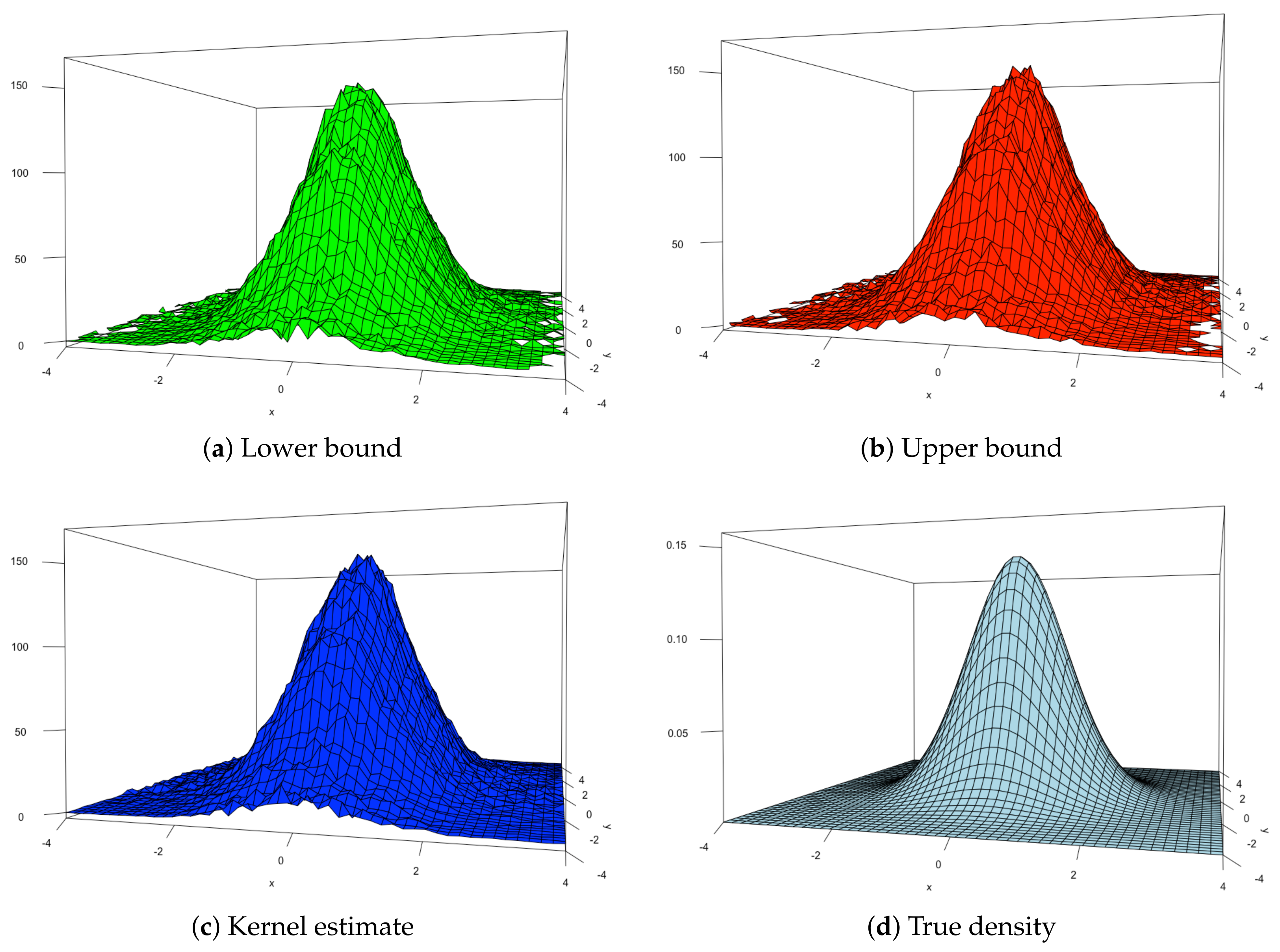
5.2. Bidimensional Case

Let θ = ( θ 1 , θ 2 ) . For k = 2 , we generate n observations X 1 = ( X 1 , 1 , X 1 , 2 ) , , X n = ( X n , 1 , X n , 2 ) from model (1) with T ( x ) = ( T 1 ( x ) , T 2 ( x ) ) , where for any x = ( x 1 , x 2 ) R 2 , T 1 ( x ) = θ 1 e 0.03 x 1 2 x 1 , T 2 ( x ) = θ 2 x 2 , V ( x ) = 1 , and f is the standard bidimensional density function. We do this for θ 1 = 0.5 , θ 2 = 0.75 .
As mentioned above, we only treat the parametric case. That is, we now assume that the functions T and V have the above parametric form with unknown θ estimated by a maximum likelihood method. Then, the kernel estimator of f is computed with a bidimensional standard Gaussian kernel. Since this can be written as a product of two univariate standard Gaussian kernels, we consider, for each of these kernels, the smoothing parameters a n , j = σ n , j n 1 5 , where σ n , j 2 is the sample variance of the X 1 , j , , X n , j , j = 1 , 2 .
Here, we take n = 800 , although smaller values give satisfactory results. For any x R 2 , f n ( x ) and its confidence bounds are computed on the basis of 1000 replications. Figure 3 shows, for the single model considered, the graph of the true density (blue color), the upper-bound graph (red), the lower-bound graph (green) and that of the estimator f n (blue). The four graphs indicate that the bidimensional Gaussian density of the noise is well estimated for the example considered.

6. Conclusions

We studied the kernel estimation of the density f of the noise in model (1) when the functions T and V are both parametric and when they are both nonparametric. In the former case, the consistency of the estimator as well as its pointwise asymptotic normality are established. This led to the construction of pointwise confidence-bound functions. It is interesting to note that from Proposition 5, Wald-type tests can be constructed for goodness-of-fit tests on f. In the case that T and V are nonparametric, only the the consistency of the estimator is studied. The main reason for this is that the study seemed to us too long and too technical.
The simulation experiment conducted shows that the estimator behaves quite well on the examples considered. It can be seen from the graphics associated with the results obtained for the parametric functions T and V that the curve of the true density function generally lies within the curves of the pointwise confidence-bound functions. Despite the fact that the pointwise asymptotic normality of f ^ n was not established (T and V are nonparametric), in light of the case where they are parametric, we wrote down the expressions of the confidence bound functions for f. It seems from the simulation results (see Figure 2) that the curve of true density is usually between those of the confidence-bound curves.

Author Contributions

Investigation, D.A.N.N. and J.S.; Methodology, J.N.-W. and M.L.; Supervision, J.N.-W.; Writing—original draft, J.N.-W., M.L. and D.A.N.N.; Writing—review & editing, J.N.-W. and M.L. Software, M.L. All authors have read and agreed to the published version of the manuscript.

Funding

This research received no external funding.

Institutional Review Board Statement

Not applicable.

Informed Consent Statement

Not applicable.

Data Availability Statement

Not applicable.

Acknowledgments

We thank the referees for their comments and suggestions, which led to an improvement of this work.

Conflicts of Interest

The authors declare no conflict of interest.

Appendix A

Appendix A.1. Theorem III.3 of Bosq and Lecoutre (1987), p. 65

Definition A1.
A kernel function K ( · ) is said to be a Geffroy kernel function if the following hold:
1.
The set of discontinuity points of K ( · ) has zero measure;
2.
The function x sup { | K ( u ) | : u x < 1 } is integrable on R k .
Some examples are the following:
1.
The indicator function I [ 1 / 2 , 1 / 2 ] is a Geffroy kernel;
2.
Any bounded variation kernel is a Geffroy kernel.
Theorem A1.
Suppose that the density function f is uniformly continuous. Let f n be the density estimator associated with any kernel K ( · ) . Then the convergence in probability
sup x R k | f n ( x ) f ( x ) | 0 , n
implies
h n 0 , n h n k log n .
Conversely, if K ( · ) is a Geffroy kernel, the condition
h n 0 , n h n k log n
implies the almost complete convergence
sup x R k | f n ( x ) f ( x ) | 0 , n .
Remark A1.
When a Geffroy kernel K ( · ) is used, the above condition on h n is equivalent to the convergence of the density estimator f n in probability, almost surely and almost completely.

Appendix A.2. Theorem V.2 of Bosq and Lecoutre (1987), p. 75

Theorem A2.
Suppose that the density function f is twice differentiable, all its partial derivatives are continuous and bounded. Let K ( · ) be an even kernel with | | y | | 2 K ( y ) d y < . Denote χ k ( x ) = 1 i , j k 2 f x i x j ( x ) t i t j K ( t ) d t . Then, under the condition h n 0 , n h n k log n , we have following asymptotic developments:
E [ f n ( x ) ] f ( x ) = h n 2 2 χ k ( x ) + o ( h n 2 ) , V a r ( f n ( x ) ) = f ( x ) n h n k K 2 + o 1 n h n k .
In consequence, we have
E { [ f n ( x ) f ( x ) ] 2 } = h n 4 4 χ k 2 ( x ) + f ( x ) n h n k K 2 + o h n 4 + 1 n h n k .

Appendix A.3. Theorem VIII.2 of Bosq and Lecoutre (1987), p. 86

Theorem A3.
Suppose that the density function f is continuous and strictly positive at distinct points t 1 , , t m R k . Let f n be the density estimator associated to a kernel K ( · ) . Then the condition h n 0 , n h n k log n implies the asymptotic normality
n h n k f n ( t i ) E f n ( t i ) ( f ( t i ) K 2 ) 1 / 2 ; 1 i m N ( 0 , I m ) ,
where N ( 0 , I m ) is the m-dimensional standard normal distribution.

Appendix A.4. Cesàro Means

Theorem A4.
Let ( a n ) be a sequence of numbers. Let
b n = a 1 + a 2 + + a n n .
If a n a , then
lim n b n = a .

References

  1. Ruppert, D.; Wand, M.; Holst, U.; Hösjer, O. Local polynomial variance-function estimation. Technometrics 1997, 39, 262–273. [Google Scholar] [CrossRef]
  2. Härdle, W.; Tsybakov, A. Local polynomial estimators of the volatility function in nonparametric autoregression. J. Econom. 1997, 81, 223–242. [Google Scholar] [CrossRef]
  3. Neumeyer, N.; Pablo, A.; Perri, F. Business cycles in emerging economies: The role of interest rates. J. Monet. Econ. 2005, 52, 345–380. [Google Scholar] [CrossRef] [Green Version]
  4. Pardo-Fernández, J.; Van Keilegom, I.; González-Manteiga, W. Testing for the equality of k regression curves. Stat. Sin. 2007, 17, 1115–1137. [Google Scholar]
  5. Dette, H.; Neumeyer, N.; Van Keilegom, I. A new test for the parametric form of the variance function in non-parametric regression. J. R. Stat. Soc. Ser. B 2007, 69, 903–917. [Google Scholar] [CrossRef] [Green Version]
  6. Neumeyer, N.; Van Keilegom, I. Estimating the error distribution in nonparametric multiple regression with applications to model testing. J. Multivar. Anal. 2010, 101, 1067–1078. [Google Scholar] [CrossRef] [Green Version]
  7. Engle, R. Autoregressive conditional heteroscedasticity with estimates of the variance of United Kingdom inflation. Econometrica 1982, 50, 987–1007. [Google Scholar] [CrossRef]
  8. Bollerslev, T.; Chou, R.; Kroner, K. ARCH modeling in finance: A review of the theory and empirical evidence. J. Econom. 1992, 52, 5–59. [Google Scholar] [CrossRef]
  9. Gourieroux, C.; Monfort, A. Qualitative threshold ARCH models. J. Econom. 1992, 52, 159–199. [Google Scholar] [CrossRef] [Green Version]
  10. Härdle, W.; Mammen, E.; Müller, M. Testing parametric versus semiparametric modeling in generalized linear models. J. Am. Stat. Assoc. 1998, 93, 1461–1474. [Google Scholar] [CrossRef]
  11. Brockwell, P.; Davis, R. Introduction to Time Series and Forecasting; Springer: Berlin/Heidelberg, Germany, 2002. [Google Scholar]
  12. Geffroy, J. Sur la convergence uniforme des estimateurs d’une densité de probabilité. Séminaire de Statistique ISUP 1973. [Google Scholar]
  13. Scott, D.; Tapia, R.; Thompson, J. Multivariate density estimation by discrete maximum penalized likelihood methods. In Graphical Representation of Multivariate Data; Elsevier: Amsterdam, The Netherlands, 1978; pp. 169–182. [Google Scholar]
  14. Deheuvels, P. Estimation non paramétrique de la densité par histogrammes généralisés. Rev. Stat. Appliquée 1977, 25, 5–42. [Google Scholar]
  15. Deheuvels, P. Non Parametric Tests of Independence. In Statistique non Paramétrique Asymptotique; Springer: Berlin/Heidelberg, Germany, 1980; pp. 95–107. [Google Scholar]
  16. Prakasa-Rao, B. Asymptotic theory for non-linear least squares estimator for diffusion processes. J. Theor. Appl. Stat. 1983, 14, 195–209. [Google Scholar] [CrossRef]
  17. Devroye, L.; Gyorfi, L. Nonparametric Density Estimation: The L1 View; Wiley: New York, NY, USA, 1985. [Google Scholar]
  18. Bosq, D.; Lecoutre, J.P. Theorie de L’estimation Fonctionnelle; Economica: Paris, France, 1987. [Google Scholar]
  19. Silverman, B. Density Estimation for Statistics and Data Analysis; Chapman and Hall: London, UK, 1986. [Google Scholar]
  20. Pearson, K. On the systematic fitting of curves to observations and measurements I, II. Biometrika 1902, 1, 265–303. [Google Scholar] [CrossRef]
  21. Pearson, K. On the systematic fitting of curves to observations and measurements I, II. Biometrika 1902, 2, 1–23. [Google Scholar] [CrossRef]
  22. Rosenblatt, M. Remark on some nonparametric estimates of a density function. Ann. Math. Statist. 1956, 27, 832–837. [Google Scholar] [CrossRef]
  23. Silverman, B.; Jones, M. E. Fix and J.L. Hodges (1951): An important contribution to nonparametric discriminant analysis and density estimation. Int. Stat. Rev. 1989, 57, 233–247. [Google Scholar] [CrossRef]
  24. Parzen, E. On estimation of a probability density function and mode. Ann. Math. Stat. 1962, 33, 1065–1076. [Google Scholar] [CrossRef]
  25. Cacoullos, T. On a Class of Admissible Partitions. Ann. Math. Stat. 1966, 37, 189–195. [Google Scholar] [CrossRef]
  26. Bierens, H. Uniform consistency of kernel estimators of a regression function under generalized conditions. J. Am. Stat. Assoc. 1983, 78, 699–707. [Google Scholar] [CrossRef]
  27. Devroye, L.; Penrod, C. Distribution-free lower bounds in density estimation. Ann. Stat. 1984, 12, 1250–1262. [Google Scholar] [CrossRef]
  28. Abdous, B. Étude d’une classe d’estimateurs à noyaux de la densité une loi de probabilité. Ph.D. Thesis, Paris, France, 1986. [Google Scholar]
  29. Tsybakov, A. Introduction to Nonparametric Estimation; Springer: Berlin/Heidelberg, Germany, 2009. [Google Scholar]
  30. Tiago de Oliveira, M. Chromatographic isolation of monofluoroacetic acid from Palicourea marcgravii St. Hil. Experientia 1963, 19, 586–587. [Google Scholar] [CrossRef] [PubMed]
  31. Heidenreich, N.B.; Schindler, A.; Sperlich, S. Bandwidth selection for kernel density estimation: A review of fully automatic selectors. Adv. Stat. Anal. 2013, 97, 403–433. [Google Scholar] [CrossRef] [Green Version]
  32. Li, Q.; Racine, J. Nonparametric Econometrics: Theory and Practice; Princeton University Press: Princeton, NJ, USA, 2007. [Google Scholar]
  33. Lecoutre, J.P. Convergence et Optimisation de Certains Estimateurs des Densités de Probabilité. Ph.D. Thesis, 1975. [Google Scholar]
  34. Chandra, S.; Taniguchi, M. Estimating functions for nonlinear time series models. Ann. Inst. Stat. Math. 2001, 53, 125–141. [Google Scholar] [CrossRef]
  35. Amano, T. Asymptotic Optimality of Estimating Function Estimator for CHARN Model. Adv. Decis. Sci. 2012, 2012, 515494. [Google Scholar] [CrossRef]
  36. Kanai, H.; Ogata, H.; Taniguchi, M. Estimating function approach for CHARN models. Metron 2010, 68, 1–21. [Google Scholar] [CrossRef]
  37. Godambe, V. An optimum property of regular maximum likelihood estimation. Ann. Math. Stat. 1960, 31, 1208–1211. [Google Scholar] [CrossRef]
  38. Godambe, V. The foundations of finite sample estimation in stochastic processes. Biometrika 1985, 72, 419–428. [Google Scholar] [CrossRef]
  39. Hansen, L. Large sample properties of generalized method of moments estimators. J. Econom. Soc. 1982, 50, 1029–1054. [Google Scholar] [CrossRef]
  40. Li, D.; Turtle, H. Semiparametric ARCH models: An estimating function approach. J. Bus. Econ. Stat. 2000, 18, 174–186. [Google Scholar]
  41. Ngatchou-Wandji, J. Estimation in a class of nonlinear heteroscedastic time series models. Electron. J. Stat. 2008, 2, 40–62. [Google Scholar] [CrossRef]
  42. Ozaki, T. Non-linear time series models for non-linear random vibrations. J. Appl. Probab. 1980, 17, 84–93. [Google Scholar] [CrossRef]
  43. Chan, K.S.; Tong, H. On the use of the deterministic Lyapunov function for the ergodicity of stochastic difference equations. Adv. Appl. Probab. 1985, 17, 666–678. [Google Scholar] [CrossRef]
  44. Al-Qassam, M.; Lane, J. Forecasting exponential autoregressive models of order 1. J. Time Ser. Anal. 1989, 10, 95–113. [Google Scholar] [CrossRef]
  45. Koul, H.L.; Schick, A. Efficient estimation in nonlinear autoregressive time-series models. Bernoulli 1997, 3, 247–277. [Google Scholar] [CrossRef]
  46. Ismail, M. Bayesian analysis of exponential AR models. Far East J. Stat. 2001, 5, 1–15. [Google Scholar]
  47. Baragona, R.; Battaglia, F.; Cucina, D. A note on estimating autoregressive exponential models. Quad. Stat. 2002, 4, 71–88. [Google Scholar]
  48. Ghosh, H.; Gurung, B.; Gupta, P. Fitting EXPAR models through the extended Kalman filter. Sankhya B 2015, 77, 27–44. [Google Scholar] [CrossRef]
  49. Rosenblatt, M. Conditional Probability Density and Regression Estimator; Academic Press: New York, NY, USA, 1969. [Google Scholar]
  50. Noda, K. Estimation of a regression function by the Parzen kernel type density estimators. Ann. Inst. Statist. Math. 1976, 28, 221–234. [Google Scholar] [CrossRef]
  51. Greblicki, W.; Krzyzak, A. Asymptotic properties of kernel estimates of a regression function. J. Stat. Plan. Inference 1980, 4, 81–90. [Google Scholar] [CrossRef]
  52. Collomb, G. Conditions nécessaires et suffisantes de convergence uniforme d’un estimateur de la régression, estimation des dérivées de la régression. CRAS 1979, A, 161–163. [Google Scholar]
  53. Nadaraya, E.A. Some new estimates for distribution functions. Theory Probab. Appl. 1964, 9, 497–500. [Google Scholar] [CrossRef]
  54. Nadaraya, E. On non-parametric estimates of density functions and regression curves. Theory Probab. Appl. 1965, 10, 186–190. [Google Scholar] [CrossRef]
  55. Devroye, L. The uniform convergence of nearest neighbor regression function estimators and their application in optimization. IEEE Trans. Inf. Theory 1978, 24, 142–151. [Google Scholar] [CrossRef] [Green Version]
  56. Devroye, L.P. The uniform convergence of the nadaraya-watson regression function estimate. Can. J. Stat. 1978, 6, 179–191. [Google Scholar] [CrossRef]
  57. Schuster, E.; Yakowitz, S. Contributions to the theory of nonparametric regression, with application to system identification. Ann. Stat. 1979, 7, 139–149. [Google Scholar] [CrossRef]
  58. Hardle, W.; Luckhaus, S. Uniform consistency of a class of regression function estimators. Ann. Stat. 1984, 12, 612–623. [Google Scholar] [CrossRef]
  59. Devroye, L.; Wagner, T. Distribution-free consistency results in nonparametric discrimination and regression function estimation. Ann. Stat. 1980, 8, 231–239. [Google Scholar] [CrossRef]
  60. Devroye, L.; Wagner, T. The strong uniform consistency of kernel density estimates. In Proceedings of the fifth International Symposium on Multivariate Analysis, New York, NY, USA, 1 January 1980; Volume 5, pp. 59–77. [Google Scholar]
  61. Spiegelman, C.; Sacks, J. Consistent window estimation in nonparametric regression. Ann. Stat. 1980, 8, 240–246. [Google Scholar] [CrossRef]
  62. Devroye, L. On the almost everywhere convergence of nonparametric regression function estimates. Ann. Stat. 1981, 9, 1310–1319. [Google Scholar] [CrossRef]
  63. Collomb, G. Estimation non paramétrique de la régression par la méthode du noyau: Propriété de convergence asymptotiquememt normale indépendante. Mathematics 1977, 65, 24–46. [Google Scholar]
  64. Collomb, G. Estimation non-paramétrique de la régression: Revue bibliographique. Int. Stat. Rev. 1981, 49, 75–93. [Google Scholar] [CrossRef]
  65. Härdle, W.; Tsybakov, A.; Yang, L. Nonparametric vector autoregression. J. Stat. Plan. Inference 1998, 68, 221–245. [Google Scholar] [CrossRef]
  66. Collomb, G.; Härdle, W. Strong uniform convergence rates in robust nonparametric time series analysis and prediction: Kernel regression estimation from dependent observations. Stoch. Process. Their Appl. 1986, 23, 77–89. [Google Scholar] [CrossRef] [Green Version]
  67. Laïb, N.; Ould-Saïd, E. A robust nonparametric estimation of the autoregression function under an ergodic hypothesis. Can. J. Stat. 2000, 28, 817–828. [Google Scholar] [CrossRef] [Green Version]
  68. Fan, J.; Yao, Q. Efficient estimation of conditional variance functions in stochastic regression. Biometrika 1998, 85, 645–660. [Google Scholar] [CrossRef] [Green Version]
  69. Linton, O.; Yan, Y. Semi-and nonparametric arch processes. J. Probab. Stat. 2011, 2011, 906212. [Google Scholar] [CrossRef] [Green Version]
  70. Franke, J.; Neumann, M.; Stockis, J.P. Bootstrapping nonparametric estimators of the volatility function. J. Econom. 2004, 118, 189–218. [Google Scholar] [CrossRef]
  71. Laïb, N. Kernel estimates of the mean and the volatility functions in a nonlinear autoregressive model with ARCH errors. J. Stat. Plan. Inference 2005, 134, 116–139. [Google Scholar] [CrossRef]
  72. Ziegelmann, F. Nonparametric estimation of volatility functions: The local exponential estimator. Econom. Theory 2002, 18, 985–991. [Google Scholar] [CrossRef]
  73. Kristensen, D. Nonparametric filtering of the realized spot volatility: A kernel-based approach. Econom. Theory 2010, 26, 60–93. [Google Scholar] [CrossRef]
  74. Zu, Y.; Boswijk, H. Estimating spot volatility with high-frequency financial data. J. Econom. 2014, 181, 117–135. [Google Scholar] [CrossRef] [Green Version]
  75. Maillot, B. Propriétés Asymptotiques de Quelques Estimateurs Non-Paramétriques Pour des Variables Vectorielles et Fonctionnelles. Ph.D. Thesis, Université du Littoral, Paris, France, 2008. [Google Scholar]
  76. Chesneau, C.; Fadili, J.; Maillot, B. Adaptive estimation of an additive regression function from weakly dependent data. J. Multivar. Anal. 2015, 133, 77–94. [Google Scholar] [CrossRef]
  77. Crambes, C.; Delsol, L.; Laksaci, A. Robust nonparametric estimation for functional data. J. Nonparametr. Stat. 2008, 20, 573–598. [Google Scholar] [CrossRef]
  78. Gheriballah, A.; Laksaci, A.; Rouane, R. Robust nonparametric estimation for spatial regression. J. Stat. Plan. Inference 2010, 140, 1656–1670. [Google Scholar] [CrossRef]
Figure 1. Kernel estimation of the density of the noise for k = 1 and parametric conditional mean and variance functions. (ad): exact density, kernel estimator, lower and upper confidence bounds curves.
Mathematics 10 00624 g001
Figure 2. Kernel estimation of the density of the noise for k = 1 and nonparametric conditional mean and variance functions. (ad): exact density, kernel estimator, lower and upper confidence bounds curves.
Mathematics 10 00624 g002
Figure 3. Kernel estimation of the density of the noise for k = 2 and parametric conditional mean and variance functions. (a): lower confidence bound curve; (b): upper confidence bound curve; (c): kernel estimate; (d): exact density.
Mathematics 10 00624 g003
Publisher’s Note: MDPI stays neutral with regard to jurisdictional claims in published maps and institutional affiliations.

