Abstract
The main task of this article is to study the patterns of mixed-mode oscillations and non-smooth behaviors in a Filippov system with external excitation. Different types of periodic spiral crossing mixed-mode oscillation patterns, i.e., “cusp-F/fold-F” oscillation, “cusp-F/two-fold/two-fold/fold-F” oscillation and “two-fold/fold-F” oscillation, are explored. Based on the analysis of the equilibrium and tangential singularities of the fast subsystem, spiral crossing oscillation around the tangential singularities is investigated. Meanwhile, by combining the fast and slow analysis methods, we can observe that the cusp, two-fold and fold-cusp singularities play an important role in generating all kinds of complex mixed-mode oscillations.
Keywords:
mixed-mode oscillations; tangential singularity; spiral crossing oscillations; external excitation MSC:
34C15; 34C05; 37G10; 37G18
1. Introduction
As a typical non-smooth dynamic system, the Filippov system reflected in the mathematical model can be expressed as discontinuous differential equations whose right-hand side is discontinuous [1]. The main motivation for studying the Filippov system comes from the fact that non-smooth factors in many practical engineering systems can be described by this kind of model, such as mechanical systems with friction [2], switched electronic systems [3], discontinuous control systems [4] and others [5,6]. Generally, a Filippov system always has a switching surface which connects two types of flows. When the trajectory touches the switching surface, the system is redefined, which can cause the qualitative changes in the system’s dynamics, such as boundary equilibrium bifurcations, multiple collision and non-smooth periodic orbit bifurcations [7,8,9,10]. Especially, the system may exhibit various types of special phenomena on the switching surface, such as sliding motion and fold, cusp, two-fold, fold-cusp tangential singularities [11,12].
On the other hand, many important practical engineering problems also involve coupling of different time scales [13,14,15,16]. This type of system may cause mixed-mode oscillations, which are formed by a relatively large excursion and nearly harmonic small amplitude oscillation during every evolution period. For example, Abdelouahab et al. [17] studied the existence of mixed-mode oscillations and canard oscillations in the neighborhoods of Hopf-like bifurcation points based on the global and local canard explosion search algorithm. Liu et al. [18] found that the folded surface and critical manifold both play an important role in the existence of mixed-mode oscillations at the folded saddle in the perturbed system. Ma et al. [19] explored the evolution mechanism of different mixed-mode oscillation patterns caused by the pitchfork bifurcation and related delay behaviors in a van der Pol–Duffing system with parameter excitation. Yu et al. [20] studied the singular Hopf bifurcation conditions and MMO behaviors in the parametric perturbed BVP system and investigated the mechanisms of two different types of MMOs using a generalized fast-slow analysis method. Chen et al. [21] explored multiple fast-slow motions, including “periodic bursts with quasi-periodic spiking”, “torus/short transient” mixed mode oscillations, “pitchfork/long transient” periodic mixed mode oscillations, amplitude-modulated and irregular oscillations from numerical method. It can be seen that the behaviors of the mixed-mode oscillation can be produced by many factors, such as different kinds of bifurcation structures [22,23], delay behaviors [24,25], and hysteresis loops [26,27]. However, most of the results about mixed-mode oscillations are made for smooth systems. When the non-smooth vector field contains multiple time scale couplings, mixed-mode oscillations may also observed. For example, Simprson et al. [28] investigated a piecewise-smooth linear FitzHugh–Nagumo system and showed that the piecewise-smooth linear model may exhibit MMO more easier than the classical FitzHugh–Nagumo model which contains a cubic polynomial as the only nonlinear term. Wang et al. [29] found that the delayed C-bifurcation leads to different types of transitions between multiple attractors, and explained the mechanism of mixed-mode oscillations in a typical Chua’s system with external excitation and a piecewise resistor. Even so, up to now, the influences of a non-smooth vector field on the vibration of mixed modes are rarely studied.
This paper investigates the mixed-mode oscillations and non-smooth dynamical behaviors in a piecewise nonlinear system with external excitation, focusing on the effects of the tangential singularities on the mixed-mode oscillations. For this purpose, we continue to analyze a realistic model in the literature [30], focusing on the effect of the external excitation. The basic circuit model with the external excitation is presented in Figure 1, where stands for the voltage source and R represents a resistive load. The voltage across R is the system output.
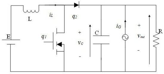
Figure 1.
The basic circuit with a periodic excitation.
The structure of the paper is set up as follows. The differential equation model of the circuit is established and the stabilities of the equilibrium and tangential singularities conditions of the fast subsystem are given in Section 2. Then, three new mixed-mode oscillation patterns, i.e., “cusp-F/fold-F” oscillation, “cusp-F/two-fold/two-fold/fold-F” oscillation and “two-fold/fold-F” oscillation are reported and the associated evolution mechanism are presented in Section 3. In Section 4, we present a brief conclusion of the paper.
2. Hybrid Model
2.1. Mathematical Model
Considering the inductor current and the voltage as state variables, the circuit described in Figure 1 can be written as
where and are either 0 or 1 and not simultaneously equal to 0 or 1, is the excitation amplitude and is the excitation frequency. The voltage output is given by , i.e.,
Considering that and , thus and the above model can be simplified as follows
By using the dimensionless transformation
the model (3) can be expressed in the form
where the new parameters are . According to Ponce and Pagano [30], a new differential equation was introduced, and the sliding control scheme can be defined as
where , and is the normalized voltage and . It can be seen that the system with the above sliding mode scheme is obtained by connecting two vector fields
according to the sign of , where . h defines the discontinuity manifold , and dividing the whole state space into two regions: one is , and the other is .
Since the excitation frequency is much less than the natural frequency, the extraneous excitation term evolves very slowly with the change of time, which indicates that the whole system has two time scales. Thus, the system can be thought of as the coupling of two subsystems, one is a slow subsystem, which is a piecewise-smooth dynamical system (6), and the other is a fast subsystem written as . Furthermore, the main characteristics of the whole system is determined by the fast subsystem, while the slow subsystem plays a moderating role in the behaviors of the whole system. Therefore, we first study the stability and bifurcation dynamics of the fast subsystem, by considering as a modulation parameter.
The equilibrium points for the vector fields and are
respectively. is a stable node (for or or stable focus (for ) since the associated eigenvalues have a negative real part, namely
Because , is an admissible stable equilibrium if , while if , is a boundary equilibrium, else is a virtual stable equilibrium. is always a admissible stable node since the associated eigenvalues are real and negative, namely , and .
2.2. Tangential Singularities
Since the fast subsystem in Equation (6) is a piecewise-smooth dynamical system, the type of contact between the smooth vector fields and the switching surface ∑ can be explained by the Lie derivatives where and denote the canonical inner product and the gradient of switching boundary function h, respectively. The m-order Lie derivatives are defined as .
The point is called tangential singularity (i.e., the orbit from is tangent to ∑) if . A point is called double tangency point (i.e., the trajectory of the smooth vector fields from is both tangent to ∑) if . The tangential sets corresponding to are given by the space lines:
It is well known that tangential singularities are important for the understanding of dynamical behaviors at a switching boundary and they form the boundaries dividing the switching surface ∑ into a crossing region and a sliding/escaping region:
Crossing regions are defined by and ;
The sliding region is defined by ;
The escaping region is defined by .
In the 3-dimensional dynamical system, two important types of generic tangential singularities that are encountered on smooth portions of ∑ are as follows:
A point is a fold point about the smooth vector field if , while , and the gradient vectors of and are linearly independent. Moreover, is a cusp point with respect to the vector field if , while , and the gradient vectors of , and are linearly independent [31].
With the same method, fold and cusp point related to the smooth vector field can also be defined. Moreover, it is possible for a point to be a double tangency point. When is a fold point, the cusp point with respect to the vector fields , is called a two fold, two-cusp singularity, respectively. If is a fold singularity with respect to one vector field and a cusp singularity with respect to the other one, we call as a fold-cusp singularity [32].
The next result summarizes the conditions of the tangential singularities which will be covered in this paper according to the parameter and fixing .
The double tangency point is given by , i.e.,
The point is a two-cusp singularity if and or a fold-cusp singularity if and (fold for , cusp for ) or (cusp for , fold for ). In the other case, the point is a two-fold singularity.
A straightforward calculation shows that the point with
and the point with
are cusp points related to and , respectively, due to the fact that and .
3. Mixed-Mode Oscillation and Its Mechanism
Based on the results of the analysis of the equilibria and the tangential singularities of Equation (6), we find that mixed-mode oscillations are obtained when the whole system undergoes a transformation between the fast system and slow system connected by the different types of tangential points on the switched surface.
In the following discussion, the parameters are always fixed and the excited frequency is fixed at . We study the evolution of the mixed-mode oscillation dynamics and the associated mechanism of the non-smooth behaviors at the switching boundary when the amplitude A is changed.
Note that is an admissible stable focus if , a boundary stable focus if or a virtual stable focus if , while is always a admissible stable node for the fixed parameters. A typical trajectory of the fast system is shown in Figure 2 for . The trajectory locally wraps around the singularity until the trajectory in the open region meets with or is near to the tangential sets and then moves to the admissible stable node .
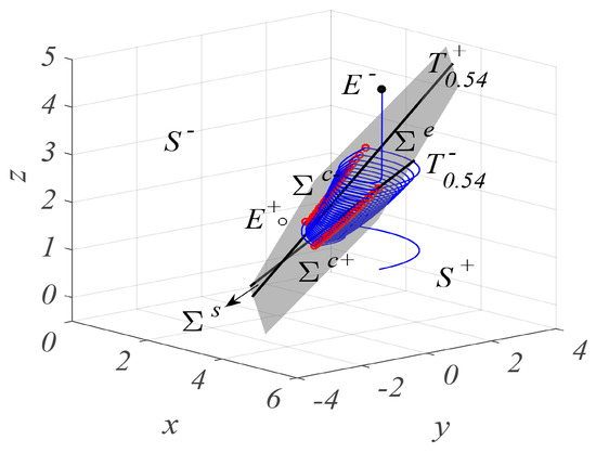
Figure 2.
is a virtual stable focus; is an admissible stable note. A typical orbit of the fast subsystem is shown: trajectories locally wrap around the tangential sets for .
3.1. Cusp-F/Fold-F Periodic Spiral Crossing Oscillation
As shown in Figure 3a, a periodic mixed-mode oscillation can be obtained when the amplitude is fixed at . It is seen that the periodic mixed-mode oscillation can be divided into two parts (seen in Figure 3b), i.e., the spiral crossing oscillation and the periodic oscillation which are connected by the tangential singularities.
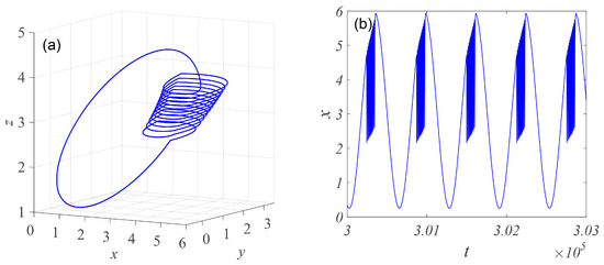
Figure 3.
A typical mixed-mode oscillation pattern for . (a) Phase portrait; (b) time series of the mixed-mode oscillation.
To explain the mechanism of this mixed-mode oscillation, Figure 4a shows the overlap of the phase portraits of different amplitudes, while Figure 4b shows the transformed phase portrait and tangential singularities with the variation of the parameter . The green line in Figure 4b refers to the two-fold singularities, the black line denotes the cusp singularities with respect to the vector field , while the black point corresponds to the fold-cusp singularity.
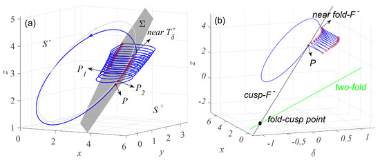
Figure 4.
(a) Stable limit cycles with (the gray orbit) and (the blue orbit); (b) overlap of the tangential singularities branches and transformed phase portrait on the .
As is shown in Figure 4a, the limit cycle (the gray orbit) with is completely in the open region and does not meet the switching boundary ∑ when it oscillates around the admissible stable node in counter-clockwise direction. When , the limit cycle (the blue orbit) contact with the switching surface ∑ at with . Based on Equation , the point P is the cusp singularity with respect to (seen in Figure 4b), which means that the trajectory in the open region is tangent to the switching boundary ∑ at P and then crosses through the switching surface ∑ to the open region governed by the vector field . Since is the virtual stable focus under the parameter conditions, the trajectory inevitably contacts with the switching surface ∑ at the point in when it scrolls down to the stable focus , then returns to the open region governed by the the admissible stable node .
In the process of moving from the the point to the stable , the trajectory may contact with the switching boundary again at in the crossing region , which may cause the trajectory to scroll down to the virtual stable focus. In this way, the trajectory may spiral around the switching surface ∑ from the cusp singularity P until the trajectory in the open region meets with or is near to the tangential sets , causing the trajectory to return back to the point P along the limit cycle in open region . We can refer to such mixed-oscillation formation as the cusp-/fold- periodic spiral crossing oscillation.
3.2. Cusp-F/Two-Fold/Two-Fold/Fold F Periodic Spiral Crossing Oscillation
When A increases from 0.92, the mixed-mode oscillation obtained in Equation (6) may exhibit some interesting behaviors. For example, Figure 5 shows a group of mixed-mode oscillation patterns in Equation (6) with increasing values of A for fixed and . It can be seen that the spiral crossing oscillation in the mixed-mode oscillation (see Figure 5a) may be divided into two parts, i.e., the left and right spiral crossing oscillation parts (see Figure 5b) with the increase of the parameter A. The corresponding phase portraits are shown in Figure 5c,d. We may find that the left trajectories may spiral around the boundary , while the right trajectories may spiral around the boundary .
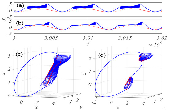
Figure 5.
Tangential singularities-induced mixed-mode oscillation patterns in Equation (6), where (the dashed line) is overlayed to give a clear view that the frequency of the periodic mixed-mode oscillation is equal to . (a,c) ; (b,d) .
The phenomenon can be also understood by the analysis of the contact between the orbit and the tangential singularities. As shown in Figure 6, when the parameter A increases from 0.92 to 1.437, the trajectories of the cusp-F/fold-F periodic spiral crossing oscillation may get to the two-fold singularity at , which imply that spiral crossing trajectories may split into two parts, i.e., the left trajectories spiraled around the boundary , and the right trajectories spiraled around the boundary , connected by two two-fold points (see in Figure 6b). We can refer to such mixed oscillation formation as the cusp-F/two-fold/two-fold/fold F periodic spiral crossing oscillation.
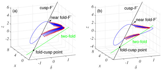
Figure 6.
Overlap of the tangential singularities branches and transformed phase portrait on the . (a) ; (b) .
3.3. Two-Fold/Fold-F Periodic Spiral Crossing Oscillation
By a further increase of parameter A, the left spiral crossing oscillation around the boundary may gradually disappear, and only the right spiral crossing oscillation is left, which still wraps around the boundary , as shown in Figure 7a for . The corresponding phase portrait is presented in Figure 7b.
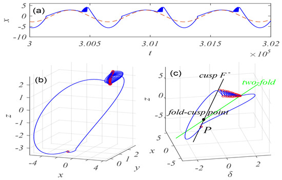
Figure 7.
A typical mixed-mode oscillation pattern for . (a) Time history; (b) phase portrait; (c) transformed phase portrait.
The mechanism analysis is obtained by the overlap of the phase diagram on the space of with the tangential singularities with the change of the parameter , as presented in Figure 7c. The mechanism can be explained simply. When A increases through 2.25, the point P where the limit cycle of the vector intersects the boundary may pass through the fold-cusp singularity (fold respect to and cusp respect to , shown in Figure 7c) along the cusp singularity at , causing the trajectory to pass through the boundary and experience a sharp turn down to the two-fold point. The trajectories of the cusp-F/two-fold/two-fold/fold F periodic spiral crossing oscillation may become unstable at , causing the left spiral crossing oscillation part to disappear (shown in Figure 5d) and evolve to a new mixed-mode oscillation pattern seen in Figure 7b. We can refer to such mixed oscillation formation as the two-fold/fold- periodic spiral crossing oscillation.
4. Conclusions
This article studies mixed-mode oscillation dynamics in a Filippov system with external excitation. When the amplitude of the excitation is changed, three new mixed-mode oscillation patterns, i.e., “cusp-F/fold-F” oscillation, “cusp-F/two-fold/two-fold/fold-F” oscillation and “two-fold/fold-F” oscillation are first reported. By regarding the excitation term as a bifurcation parameter, the stabilities of the (admissible and boundary) equilibrium and the conditions of different types of tangential points, such as cusp, two-fold and fold-cusp singularity, are explored. With the decrease of the excitation amplitude, when the excitation term passes through the two-fold point, the periodic spiral crossing oscillation may become unstable and a periodic oscillation with two (left and right) spiral crossing trajectories is created. When the excitation term passes through the fold-cusp point, the left spiral crossing trajectory of the periodic oscillation may suddenly disappear and only the right spiral crossing trajectory is left. Besides, the results proposed in this paper are advantageous to understand the mixed-mode oscillation in non-smooth dynamical systems. Our further work will focus on the effect of the different behaviors of mixed-mode oscillation caused by various switched scheme and the potential applications on Filippov system.
Author Contributions
Formal analysis, C.Z.; methodology, C.Z. and Q.T.; writing—original draft preparation, Q.T.; writing—review and editing, C.Z. All authors have read and agreed to the published version of the manuscript.
Funding
This work is supported by the National Natural Science Foundation of China (Grant Nos. 11502091 and 11801209).
Institutional Review Board Statement
Not applicable.
Informed Consent Statement
Not applicable.
Data Availability Statement
Not applicable.
Acknowledgments
We would like to express our deep thanks to the anonymous referees for their valuable comments.
Conflicts of Interest
The author declares no conflict of interest.
References
- Filippov, A.F. Differential Equations with Discontinuous Righthand Sides. In Mathematics and Its Applications; Soviet Series; Arscott, F.M., Ed.; Springer: Dordrecht, The Netherlands; Kluwer Academic: Boston, MA, USA, 1988. [Google Scholar]
- Polekhin, I. On Montions without falling of an interted pendulum with dry friction. J. Geom. Mech. 2018, 10, 411–417. [Google Scholar] [CrossRef]
- Meo, S.; Toscano, L. On the existence and uniqueness of the ODE solution and its approximation using the means averaging approach for the class of power electronic converters. Mathematics 2021, 10, 1146. [Google Scholar] [CrossRef]
- Baier, R.; Braun, P.; Grune, L.; Kellett, C.M. Numerical calculation of nonsmooth control lyapunov functions via piecewise affine approximation. IFAC-PapersOnLine 2019, 52, 370–375. [Google Scholar] [CrossRef]
- Bhattacharyya, J.; Roelke, D.L.; Pal, S.; Banerjee, S. Sliding mode dynamics on a prey-predator system with intermittent harvesting policy. Nonlinear Dyn. 2019, 98, 1299–1314. [Google Scholar] [CrossRef]
- Popov, M. Friction under large-amplitude normal oscillations. Facta Univ.-Ser. Mech. Eng. 2021, 19, 105–113. [Google Scholar] [CrossRef]
- Antali, M.; Stepan, G. Sliding and crossing dynamics in extended Filippov systemsm. SIAM J. Appl. Dyn. Syst. 2018, 17, 823–858. [Google Scholar] [CrossRef]
- Walsh, J.; Widiasih, E. A discontinuous ODE model of the glacial cycles with diffusive heat transport. Mathematics 2021, 8, 316. [Google Scholar] [CrossRef]
- Althubiti, S.; Aldawish, I.; Awrejcewicz, J.; Bazighifan, O. New oscillation results of even-order emden-fowler neutral differential equations. Symmetry 2021, 13, 2177. [Google Scholar] [CrossRef]
- Santra, S.S.; Alotaibi, H.; Noeiaghdam, S.; Sidorov, D. On nonlinear forced impulsive differential equations under canonical and non-canonical conditions. Symmetry 2021, 13, 2066. [Google Scholar] [CrossRef]
- Freire, E.; Ponce, E.; Torres, F. On the critical crossing cycle bifurcation in planar Filippov systems. J. Differ. Equ. 2015, 259, 7086–7107. [Google Scholar] [CrossRef]
- Cristiano, R.; Pagano, D.J. Two-parameter boundary equilibrium bifurcations in 3D-Filippov systems. J. Nonlinear Sci. 2019, 29, 2845–2875. [Google Scholar] [CrossRef]
- Han, X.J.; Zhang, Y.; Bi, Q.S.; Kurths, J. Two novel bursting patterns in the Duffing system with multiple-frequency slow parametric excitations. Chaos 2018, 28, 043111. [Google Scholar] [CrossRef] [PubMed]
- Yu, Y.; Zhang, Z.D.; Han, X.J. Periodic or chaotic bursting dynamics via delayed pitchfork bifurcation in a slow-varying controlled system. Commun. Nonlinear Sci. Numer. Simul. 2018, 56, 380–391. [Google Scholar] [CrossRef]
- Ma, X.D.; Jiang, W.A.; Zhang, X.F.; Han, X.J.; Bi, Q.S. Complex bursting dynamics of a Mathieu-van der Pol-Duffing energy harvester. Phys. Scr. 2021, 96, 015213. [Google Scholar] [CrossRef]
- Duan, L.X.; Liang, T.T.; Zhao, Y.Q.; Xi, H.G. Multi-time scale dynamics of mixed depolarization block bursting. Nonlinear Dyn. 2021, 103, 1043–1053. [Google Scholar] [CrossRef]
- Abdelouahab, M.S.; Lozi, R. Hopf-like bifurcation and mixed mode oscillation inn a fractional-order FitzHugh-Nagumo model. In Proceedings of the Third International Conference of Mathematical Sciences, Istanbul, Turkey, 4–8 September 2019; Volume 2183, p. 100003. [Google Scholar]
- Liu, Y.R.; Lu, S.Q.; Lu, B.; Kurths, J. Mixed-mode oscillations for slow-fast perturbed systems. Phys. Scr. 2021, 96, 125258. [Google Scholar] [CrossRef]
- Ma, X.D.; Yu, Y.; Wang, L.F. Complex mixed-mode vibration types triggered by the pitchfork bifurcation delay in a driven van der Pol-Duffing oscillator. Appl. Math. Comput. 2021, 411, 126522. [Google Scholar] [CrossRef]
- Yu, Y.; Zhang, C.; Chen, Z.Y.; Zhang, Z.D. Canard-Induced Mixed Mode Oscillations as a Mechanism for the Bonhoeffer-van der Pol Circuit under Parametric Perturbation; Emerald Publishing Limited: Bingley, UK, 2021. [Google Scholar] [CrossRef]
- Chen, Z.Y.; Chen, F.Q.; Zhou, L.Q. Slow-fast motions induced by multi-stability and strong transient effects in an accelerating viscoelastic beam. Nonlinear Dyn. 2021, 106, 45–66. [Google Scholar] [CrossRef]
- Wojcik, J.; Shilnikov, A. Voltage interval mappings for activity transitions in neuron models for elliptic bursters. Phys. D Nonlinear Phenom. 2011, 240, 1164–1180. [Google Scholar] [CrossRef]
- Zhang, C.; Bi, Q.S. On two-parameter bifurcation analysis of the periodic parameter-switching Lorenz oscillator. Nonlinear Dyn. 2015, 81, 577–583. [Google Scholar] [CrossRef]
- Yue, Y.; Han, X.J.; Zhang, C.; Bi, Q.S. Mixed-mode oscillations in a nonlinear time delay oscillator with time varying parameters. Commun. Nonlinear Sci. Numer. Simul. 2017, 47, 23–34. [Google Scholar] [CrossRef]
- Karamchandani, A.J.; Graham, J.N.; Riecke, H. Pulse-coupled mixed-mode oscillators: Cluster states and extreme noise sensitivity. Chaos 2018, 28, 043115. [Google Scholar] [CrossRef] [PubMed]
- Meng, P.; Wang, Q.Y.; Lu, Q.S. Bursting synchronization dynamics of pancreatic β-cells with electrical and chemical coupling. Cogn. Neurodyn. 2013, 7, 197–212. [Google Scholar] [CrossRef][Green Version]
- Han, X.J.; Bi, Q.S.; Zhang, C.; Yue, Y. Delayed bifurcations to repetitive spiking and classifcation of delay-induced bursting. Int. J. Bifurc. Chaos 2014, 24, 1450098. [Google Scholar] [CrossRef]
- Simpson, D.J.W.; Kuske, R. Mixed-mode oscillations in a stochastic piecewise-linear system. Phys. D Nonlinear Phenom. 2011, 240, 1189–1198. [Google Scholar] [CrossRef][Green Version]
- Wang, Z.X.; Zhang, Z.D.; Bi, Q.S. Bursting oscillations with delayed C-bifurcations in a modified Chua’s circuit. Nonlinear Dyn. 2020, 100, 2899–2915. [Google Scholar] [CrossRef]
- Ponce, E.; Pagano, D.J. Chaos through sliding bifurcations in a boost converter under a SMC strategy. IFAC Proc. Vol. 2009, 42, 279–284. [Google Scholar] [CrossRef]
- Jeffrey, M.R.; Colombo, A. The two-fold singularity of discontinuous vector fields. SIAM J. Appl. Dyn. Syst. 2009, 8, 624–640. [Google Scholar] [CrossRef]
- de Carvalho, T.; Teixeira, M.A. Basin of attraction of a cusp-fold singularity in 3D piecewise smooth vector fields. J. Math. Anal. Appl. 2014, 418, 11–30. [Google Scholar] [CrossRef]


Publisher’s Note: MDPI stays neutral with regard to jurisdictional claims in published maps and institutional affiliations. |
© 2022 by the authors. Licensee MDPI, Basel, Switzerland. This article is an open access article distributed under the terms and conditions of the Creative Commons Attribution (CC BY) license (https://creativecommons.org/licenses/by/4.0/).