Generalized Type-2 Fuzzy Control for Type-I Diabetes: Analytical Robust System

Abstract

The insulin injection rate in type-I diabetic patients is a complex control problem. The mathematical dynamics for the insulin/glucose metabolism can be different for various patients who undertake different activities, have different lifestyles, and have other illnesses. In this study, a robust regulation system on the basis of generalized type-2 (GT2) fuzzy-logic systems (FLSs) is designed for the regulation of the blood glucose level. Unlike previous studies, the dynamics of glucose–insulin are unknown under high levels of uncertainty. The insulin-glucose metabolism has been identified online by GT2-FLSs, considering the stability criteria. The learning scheme was designed based on the Lyapunov approach. In other words, the GT2-FLSs are learned using adaptation rules that are concluded from the stability theorem. The effect of the dynamic estimation error and other perturbations, such as patient activeness, were eliminated through the designed adaptive fuzzy compensator. The adaptation laws for control parameters, GT2-FLS rule parameters, and the designed compensator were obtained by using the Lyapunov stability theorem. The feasibility and accuracy of the designed control scheme was examined on a modified Bergman model of some patients under different conditions. The simulation results confirm that the suggested controller has excellent performance under various conditions.

1. Introduction

Through the development of electronic devices and sensors, modern control systems are extensively used in medical applications. One of the challenging problems is the glucose regulation of type-I diabetes (T1D). Many people all over the world are suffering from this illness. In T1D, the pancreas cannot produce enough insulin, and then the blood glucose exceeds the desired range. Insulin is a vital hormone which supports the body’s cells in its slow conversion from glucose into energy. When conversion does not happen, the blood glucose level increases and it can reach a dangerous level. The patients with this condition should always inject insulin to stay alive [1,2].

The control systems for this problem can be categorized into three classes: No-sensor (open-loop) control systems, classical controllers, and neuro-fuzzy control systems. In the first case, the insulin is injected by a predefined plan [3]. The main drawback of these methods is that the insulin injection plan can be different form one patient to another. Additionally, the effect of other illnesses of patients and other unpredicted activities are not considered. Generally, these methods do not result in the desired performance [4].

The classic controllers that are frequently used for glucose regulation can be classified into three cases: PID controllers, sliding mode controllers (SMCs), and model-based predictive controllers (MPCs). For the PID control scheme, various approaches have been presented for optimization of the PID gains. For example, in the Ref. [5], the PID controller was optimized by the Grasshopper optimization technique, and the quantity of injection times was investigated. In the Ref. [6], the various approaches were reviewed, and the effect of meal conditions was investigated. In the Ref. [7], the fractional-order PID was designed and its performance was studied in comparison with integer-order PID. Similar to the Ref. [7], the genetic algorithm was employed in the Ref. [8] to adjust the fractional-order PID controller, and the Bergman minimal model was employed for evaluation. Various versions of the SMC scheme have been applied to the glucose regulation problem. For example, the simple SMC scheme was developed in the Refs. [9,10] for glucose regulation. In the Ref. [11], the output feedback SMC was designed to retain the glucose value in a desired level, and its performance was compared with the open-loop approaches. In the Ref. [12], the particle-swarm optimization scheme was used to tune a SMC scheme, and it was shown that the glucose level was kept near to the desired range. The terminal SMC was developed in the Ref. [13], and the effect of mathematical uncertainties was analyzed. The other control system which has frequently been reported in the literature for glucose regulation is the MPC system [14]. Generally, the MPC methods result in better performance than the approaches discussed above.

In most of the aforementioned studies, the controller was designed on the basis of the Bergman model. To tackle the effects of an uncertain model, some fuzzy logic controllers (FLCs) have been developed [15,16]. In this class of controllers, fuzzy logic systems (FLSs) are often combined with the above-discussed controllers to estimate the uncertainties. For example, in the Ref. [17], a FLS was used in the SMC scheme to develop the regulation performance. An FLS approach based on a deep learned scheme was suggested in the Ref. [18] to predict the glucose level in a long-term horizon. In the Ref. [19], the FLSs were used to estimate some uncertain functions in the Bergman model. In the Ref. [20], the blood glucose situation was analyzed by FLSs, and the suitable insulin level was determined by the FLS model. In the Ref. [21], an artificial pancreas was designed by the use of FLSs, and better performance of the FLS model was shown in comparison with the Bergman model.

The interval type-2 FLSs (IT2-FLSs) outperformed in comparison with the type-I counterparts [22,23]. In a few studies, IT2-FLSs have been used in glucose regulation problems. For example, the nephropathy predicting the use of type-2 FLCs was investigated in the Ref. [24]. In the Ref. [25], the IT2-FLSs were used for the estimation of glucose–insulin dynamics, and the controller was designed on the basis of a fuzzy model. The backstepping control scheme was developed by IT2-FLSs in the Ref. [26], and the better performance of type-2 FLSs was shown. The diet recommendation system was designed in the Ref. [27] by IT2-FLSs. In the Ref. [20], an IT2-FLS-based controller was designed, and the effect of blood sugar was investigated. In the Ref. [28], the glucose level was predicted, and then on the basis of the glucose level, the rate of insulin injection was determined by IT2-FLSs. In the Ref. [29], the changes of model parameters were taken into account, and a IT2-FLS-based controller was designed and the better performance of IT2-FLSs was validated.

Recently, generalized type-2 FLSs have been developed to achieve better performance in noisy complicated problems [30]. The superiority of GT2-FLSs compared to their conventional counterparts has been shown in engineering problems, such as medical systems [31], classification problems [32], financial systems [33], control systems [34], modeling applications [35], forecasting problems [36], and education systems [37], among many others.

The review of previous studies has shown that some issues in this problem need to be studied further.

• In most of the aforementioned studies, the controllers were designed by the use of a simple Bergman model. However, the mathematical model of glucose–insulin in various conditions may be unreliable.
• Some conventional approaches do not have any stability guarantee.
• In most studies, the evolutionary-based methods are employed for controller learning that imposes a high computational cost without any stability criteria.
• In most other stable and robust controllers, such as SMCs, the minimal Bergman model is used and strong dynamic perturbations are neglected. Additionally, the Bergman mathematical model is used in the controller design.
• The speed of glucose regulation in most studies is not desirable enough, and needs to be studied further.

Then, the main questions of the study are as follows:

• How can we design a controller that does not depend on metabolism?
• How can we improve robustness against the meal effect, patient activities, and other perturbations, such as the unknown illnesses of patients?
• How can modeling of the metabolism be improved, considering all uncertainties?

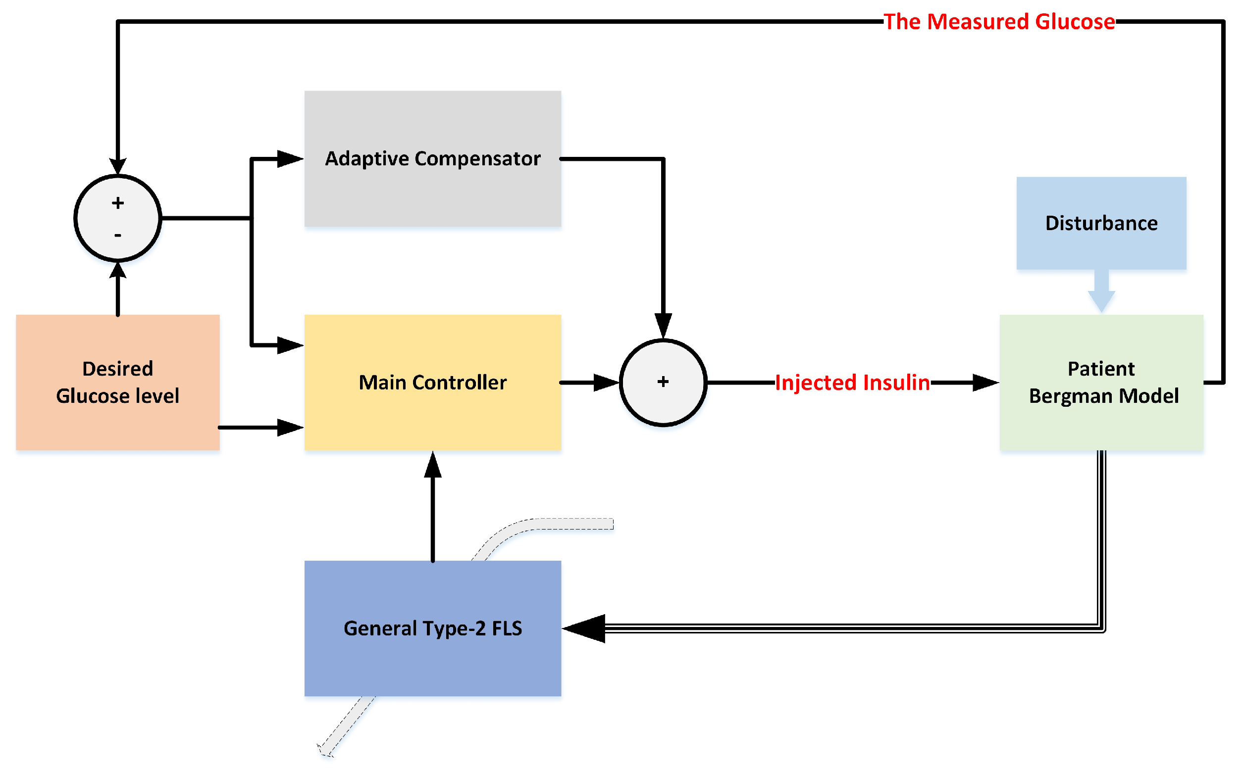
From the above motivations, we designed a robust control system. The dynamics of insulin/glucose were completely unknown in the schemed approach. The uncertainties were online-approximated by the suggested GT2-FLS. The suggested GT2-FLS was online-tuned such that the insulin/glucose dynamic was stable and the glucose level reached the desired level. The effects of perturbations were compensated by the designed adaptive compensator. The main advantages of this study are:

• The insulin/glucose metabolism is considered to be unknown.
• An effective GT2-FLS with better estimation accuracy is developed for online metabolism estimation.
• The suggested GT2-FLS is optimized at every glucose measurement considering the dynamic stability criteria.
• The challenging conditions, such as dynamic perturbation by noisy signals, meal effect, and estimation errors are taken into account, and an adaptive fuzzy compensator is designed.

2. System Description and Problem Statement

Diabetes is a metabolic issue which is mainly classified into two categories: type-I and type-II diabetes. The autoimmune reaction of type-I diabetic patients destructs the beta cells, and consequently, insulin production is reduced. In type-II diabetes, the body is resistant to insulin. In general, in diabetes of any type, cells are unable to convert carbohydrates into energy needed by the body, leading to high blood glucose concentrations or hyperglycemia. Consistently high blood glucose levels over a long time can lead to chronic consequences, such as heart disease, kidney failure, blindness, stroke, and amputation. On the other hand, injecting a high dose of insulin into a diabetic patient causes a severe drop in blood glucose concentration or hypoglycemia, which can lead to anesthesia, coma, and even death in the diabetic patient. Glucose control is a vital problem in type-I diabetes.

The modified Bergman is frequently used for examination of the glucose control systems. This model has a complete structure that includes meal effects and patients’ daily activities. The system dynamics are given as [38]:

$$\begin{array}{c}\dot{G}=d_a-G\left(\chi +{\pi }_1\right)+g_b{\pi }_1\hfill \\ \dot{\chi }={\pi }_3\left(\iota -{\iota }_b\right)-\chi {\pi }_2\hfill \\ \dot{\iota }=k_f{\iota }_b+\varphi b_f\hfill \\ \dot{\varphi }=-k_s\varphi +u\hfill \\ {\dot{R}}_1=-\left(R_1-d\right)C_1\hfill \\ {\dot{R}}_2=-\left(R_2-R_1\right)C_2\hfill \end{array}$$

(1)

where $C_1$, $C_2$, $g_b$, ${\iota }_b$, $k_f$, $k_s$, $k_{gr}$${\pi }_1$, ${\pi }_2$ and ${\pi }_3$ are positive constants. $d_a$ represents the rate of glucose metabolism. G ($mg/dL$) and $\iota$ ($mIU$) are the glucose and insulin levels in blood. $R_1$ and $R_2$ denote the impact of meals on blood glucose. The system dynamics are rewritten as:

$$\begin{array}{c}{\dot{y}}_1=f_1+{\epsilon }_1-y_1{y}_2,\hfill \\ f_1=-{\pi }_1\left(y_1-g_b\right),\hfill \\ {\epsilon }_1=w_1+k_{gr}{y}_5\hfill \end{array}$$

(2)

$$\begin{array}{c}{\dot{y}}_2=f_2+{\epsilon }_2+{\pi }_3{y}_3,\hfill \\ f_2=-{\pi }_2{y}_2-{\pi }_3{\iota }_b,\hfill \\ {\epsilon }_2=w_2\hfill \end{array}$$

(3)

$$\begin{array}{c}{\dot{y}}_3=f_3+{\epsilon }_3+b_f{y}_4,\hfill \\ f_3=-k_f{y}_3,\hfill \\ {\epsilon }_3=w_3\hfill \end{array}$$

(4)

$$\begin{array}{c}{\dot{y}}_4=f_4+{\epsilon }_4+u,\hfill \\ f_4=-k_s{y}_4,\hfill \\ {\epsilon }_4=w_4\hfill \end{array}$$

(5)

where $y_5$ is defined as $y_5={k_g}_r{R}_2$, and $w_i,i=1,\dots ,5$ are dynamic perturbations. The system dynamics are estimated as:

$$\begin{array}{c}{\widehat{y}}_1^{\left(4\right)}=\widehat{f}\left(\chi |\theta \right)-\widehat{g}{y}_{1}u\hfill \\ -{\kappa }_1{\widehat{\upsilon }}^{\left(3\right)}-{\kappa }_2{\widehat{\upsilon }}^{\left(2\right)}-{\kappa }_3\dot{\widehat{\upsilon }}-{\kappa }_4\widehat{\upsilon }\hfill \end{array}$$

(6)

where $\widehat{f}\left(\chi |\theta \right)$ is the proposed FLS and $\chi ={[y_1,D_t^q{y}_1]}^T$ denotes the input vector of GT2-FLS, and $D_t^q{y}_1$ represents the fractional derivative of $y_1$ by order q. The ${\kappa }_i,i=1,\dots ,4$ were chosen such that the polynomial $s^4+{\kappa }_1{s}^3+{\kappa }_2{s}^2+{\kappa }_{3}s+{\kappa }_4$ became Hurwitz-stable. The estimated error was defined as $\widehat{\upsilon }={\widehat{y}}_1-y_1$. The control objective is that the system output is stabilized and converged to the normal level. Figure 1 displays the general scheme of the suggested controller. A detailed diagram is given in Figure 2.

3. Generalized Type-2 FLS

The glucose–insulin metabolism is a complicated dynamic system because it is perturbed by various unknown factors, such as unpredicted activities, the unknown effect of various meals, and the effect of a broad range of other illnesses. Regarding the high level of uncertainties in the glucose–insulin metabolism, in this paper, a new generalized FLS is suggested for modeling the dynamics. The generalized type-2 FLSs are the developed versions of interval type-2 FLSs. In GT2-FLS, the secondary memberships are not fixed values, but they are different at each primary membership. The main approach to formulate the GT2-FLSs is the use of the $\alpha$-planes approach [39]. In this method, a general MF is represented by some horizontal slices (see Figure 3).

The glucose–insulin metabolism is identified using a GT2-FLS. In other words, by the use GT2-FLS, the dynamics of the glucose level is modeled, and then the suitable insulin rate is determined. The schematic of GT2-FLS is presented in Figure 4. The details are provided below [30].

Input layer: The inputs are considered to be $y_1\left(t\right)$ and $D_t^q{y}_1\left(t\right)$.

Membership layer: Each node of a membership layer represents a membership function (MF). Three Gaussian MFs are considered as $A_i^j$, $i=1,2$, and $j=1,2,3$ (the $jth$ MF for the $ith$ input). The memberships are calculated as:

$$\begin{array}{c}{\overline{\mu }}_{{\tilde{A}}_{1,{\alpha }_h}^1}\left(y_1\left(t\right)\right)=exp\left(-\frac{1}{2}{\left(\frac{y_1\left(t\right)-{\overline{y}}_1}{{{\overline{\sigma }}_{{\alpha }_h}}^2}\right)}^2\right)\hfill \\ {\underline{\mu }}_{{\tilde{A}}_{1,{\alpha }_h}^1}\left(y_1\left(t\right)\right)=exp\left(-\frac{1}{2}{\left(\frac{y_1\left(t\right)-{\overline{y}}_1}{{\underline{\sigma }}^2}\right)}^2\right)\hfill \end{array}$$

(7)

$$\begin{array}{c}{\overline{\mu }}_{{\tilde{A}}_{1,{\alpha }_h}^2}\left(y_1\left(t\right)\right)=exp\left(-\frac{1}{2}{\left(\frac{y_1\left(t\right)}{{{\overline{\sigma }}_{{\alpha }_h}}^2}\right)}^2\right)\hfill \\ {\underline{\mu }}_{{\tilde{A}}_{1,{\alpha }_h}^2}\left(y_1\left(t\right)\right)=exp\left(-\frac{1}{2}{\left(\frac{y_1\left(t\right)}{{{\underline{\sigma }}_{{\alpha }_h}}^2}\right)}^2\right)\hfill \end{array}$$

(8)

$$\begin{array}{c}{\overline{\mu }}_{{\tilde{A}}_{1,{\alpha }_h}^3}\left(y_1\left(t\right)\right)=exp\left(-\frac{1}{2}{\left(\frac{y_1\left(t\right)-{\underline{y}}_1}{{{\overline{\sigma }}_{{\alpha }_h}}^2}\right)}^2\right)\hfill \\ {\underline{\mu }}_{{\tilde{A}}_{1,{\alpha }_h}^3}\left(y_1\left(t\right)\right)=exp\left(-\frac{1}{2}{\left(\frac{y_1\left(t\right)-{\underline{y}}_1}{{{\underline{\sigma }}_{{\alpha }_h}}^2}\right)}^2\right)\hfill \end{array}$$

(9)

where ${\overline{y}}_1$/${\underline{y}}_1$ denotes the upper/lower bounds for the glucose level. Similarly, the memberships for the second input are computed as:

$$\begin{array}{c}{\overline{\mu }}_{{\tilde{A}}_{2,{\alpha }_h}^1}\left(D_t^q{y}_1\left(t\right)\right)=exp\left(-\frac{1}{2}{\left(\frac{D_t^q{y}_1\left(t\right)-{{\overline{y}}^{\prime }}_1}{{{\overline{\sigma }}_{{\alpha }_h}}^2}\right)}^2\right)\hfill \\ {\underline{\mu }}_{{\tilde{A}}_{2,{\alpha }_h}^1}\left(D_t^q{y}_1\left(t\right)\right)=exp\left(-\frac{1}{2}{\left(\frac{D_t^q{y}_1\left(t\right)-{{\overline{y}}^{\prime }}_1}{{{\underline{\sigma }}_{{\alpha }_h}}^2}\right)}^2\right)\hfill \end{array}$$

(10)

$$\begin{array}{c}{\overline{\mu }}_{{\tilde{A}}_{2,{\alpha }_h}^2}\left(D_t^q{y}_1\left(t\right)\right)=exp\left(-\frac{1}{2}{\left(\frac{D_t^q{y}_1\left(t\right)}{{{\overline{\sigma }}_{{\alpha }_h}}^2}\right)}^2\right)\hfill \\ {\underline{\mu }}_{{\tilde{A}}_{2,{\alpha }_h}^2}\left(D_t^q{y}_1\left(t\right)\right)=exp\left(-\frac{1}{2}{\left(\frac{D_t^q{y}_1\left(t\right)}{{{\underline{\sigma }}_{{\alpha }_h}}^2}\right)}^2\right)\hfill \end{array}$$

(11)

$$\begin{array}{c}{\overline{\mu }}_{{\tilde{A}}_{2,{\alpha }_h}^3}\left(D_t^q{y}_1\left(t\right)\right)=exp\left(-\frac{1}{2}{\left(\frac{D_t^q{y}_1\left(t\right)-{{\underline{y}}^{\prime }}_1}{{{\overline{\sigma }}_{{\alpha }_h}}^2}\right)}^2\right)\hfill \\ {\underline{\mu }}_{{\tilde{A}}_{2,{\alpha }_h}^3}\left(D_t^q{y}_1\left(t\right)\right)=exp\left(-\frac{1}{2}{\left(\frac{D_t^q{y}_1\left(t\right)-{{\underline{y}}^{\prime }}_1}{{{\underline{\sigma }}_{{\alpha }_h}}^2}\right)}^2\right)\hfill \end{array}$$

(12)

where ${{\underline{y}}^{\prime }}_1$ and ${{\overline{y}}^{\prime }}_1$ are the lower and upper boundaries for the glucose level.

Rules layer: The output of the rule layer is written as:

$$\begin{array}{c}{\underline{z}}_1={\underline{\mu }}_{A_1^1}{\underline{\mu }}_{A_2^1},{\underline{z}}_2={\underline{\mu }}_{A_1^1}{\underline{\mu }}_{A_2^2},{\underline{z}}_3={\underline{\mu }}_{A_1^1}{\underline{\mu }}_{A_2^3}\hfill \\ {\underline{z}}_4={\underline{\mu }}_{A_1^2}{\underline{\mu }}_{A_2^1},{\underline{z}}_5={\underline{\mu }}_{A_1^2}{\underline{\mu }}_{A_2^2},{\underline{z}}_6={\underline{\mu }}_{A_1^2}{\underline{\mu }}_{A_2^3}\hfill \\ {\underline{z}}_7={\underline{\mu }}_{A_1^3}{\underline{\mu }}_{A_2^1},{\underline{z}}_8={\underline{\mu }}_{A_1^3}{\underline{\mu }}_{A_2^2},{\underline{z}}_9={\underline{\mu }}_{A_1^3}{\underline{\mu }}_{A_2^3}\hfill \end{array}.$$

(13)

The upper firing degrees are calculated as:

$$\begin{array}{c}{\overline{z}}_1={\overline{\mu }}_{A_1^1}{\overline{\mu }}_{A_2^1},{\overline{z}}_2={\overline{\mu }}_{A_1^1}{\overline{\mu }}_{A_2^2},{\overline{z}}_3={\overline{\mu }}_{A_1^1}{\overline{\mu }}_{A_2^3}\hfill \\ {\overline{z}}_4={\overline{\mu }}_{A_1^2}{\overline{\mu }}_{A_2^1},{\overline{z}}_5={\overline{\mu }}_{A_1^2}{\overline{\mu }}_{A_2^2},{\overline{z}}_6={\overline{\mu }}_{A_1^2}{\overline{\mu }}_{A_2^3}\hfill \\ {\overline{z}}_7={\overline{\mu }}_{A_1^3}{\overline{\mu }}_{A_2^1},{\overline{z}}_8={\overline{\mu }}_{A_1^3}{\overline{\mu }}_{A_2^2},{\overline{z}}_9={\overline{\mu }}_{A_1^3}{\overline{\mu }}_{A_2^3}\hfill \end{array}$$

(14)

Type reduction layer: The output is obtained by the use of a Nie–Tan-type reduction, as [40]:

$$z_{l,{\alpha }_h}=\frac{{\alpha }_h}{{\displaystyle \sum _{h=1}^H}{\alpha }_h}\frac{{\overline{z}}_{l,{\alpha }_h}+{\underline{z}}_{l,{\alpha }_h}}{{\displaystyle \sum _{l=1}^M}{\overline{z}}_{l,{\alpha }_h}+{\underline{z}}_{l,{\alpha }_h}}$$

(15)

where M and H are the number of rules and slices, respectively.

The output layer: The output signal is written as:

$$\widehat{f}=\sum _{l=1}^M\sum _{l=1}^M{z}_{l,{\alpha }_h}{\theta }_{l,{\alpha }_h}$$

(16)

where ${\theta }_{l,{\alpha }_h},l=1,\dots ,M,h=1,\dots ,H$ are the rule section parameters.

Remark 1.

The rules are optimized by the online stable learning laws (18). However, the MF parameters are fixed. It should be noted that the upper and lower bounds of MFs are chosen on the basis of the input variation range.

4. Controller Design

As shown in the block diagram of Figure 2, the modified Bergman model is employed to evaluate the designed controller. The parameters of the Bergman model are different from one patient to another. Additionally, this model can be perturbed by various factors, such as patient activities, meal effects, and other diseases of the diabetic patient. Then, to model the uncertainties, the designed GT2-FLS is suggested. Using the GT2-FLS, the glucose–insulin metabolism is modeled. The suggested fuzzy model is not fixed, but it is adaptively changed based on the glucose measurement information. The GT2-FLS is optimized by learning rules that ensure the stability. By the estimated model, the regulation system is designed that guarantees global stability. To ensure the asymptotic stability, an adaptive compensator is also designed. The compensator works with the main controller in parallel. The main results are given in two theorems. First, the global stability is investigated, and then the compensator is designed.

Theorem 1.

Considering the control signal (17) and adaptive learning rules (18), the closed-loop glucose–insulin system is globally stable.

$$u=-\frac{1}{\widehat{g}{y}_1}\left(-\widehat{f}+r^{\left(4\right)}-k^T\underline{\upsilon }+{\kappa }^T\underline{\widehat{\upsilon }}\right)$$

(17)

$$\begin{array}{c}\dot{\theta }=\gamma {\underline{\widehat{\upsilon }}}^T{\pi }_{2}bZ\hfill \\ \dot{\widehat{g}}=\gamma {\underline{\widehat{\upsilon }}}^T{\pi }_{2}b{y}_{1}u\hfill \end{array}$$

(18)

where $\gamma$ represents the learning rate, r is the glucose signal, and ${\pi }_i,i=1,2$ are positive definite matrices, such that:

$$A^T{\pi }_1+{\pi }_{1}A=-Q_1$$

(19)

$${\mathrm{\Lambda }}^T{\pi }_2+{\pi }_2\mathrm{\Lambda }=-Q_2$$

(20)

where

$$\mathrm{\Lambda }=\left[\begin{array}{cccc}0& 1& 0& 0\\ 0& 0& 1& 0\\ 0& 0& 0& 1\\ -{\kappa }_4& -{\kappa }_3& -{\kappa }_2& -{\kappa }_1\end{array}\right]$$

(21)

$$A=\left[\begin{array}{cccc}0& 1& 0& 0\\ 0& 0& 1& 0\\ 0& 0& 0& 1\\ -k_4& -k_3& -k_2& -k_1\end{array}\right]$$

(22)

$$b=\left[\begin{array}{c}0\\ 0\\ 0\\ 1\end{array}\right]$$

(23)

$$\underline{\upsilon }=\left[\begin{array}{c}\upsilon \\ \dot{\upsilon }\\ \ddot{\upsilon }\\ {\upsilon }^{\left(3\right)}\end{array}\right]$$

(24)

$$\underline{\widehat{\upsilon }}=\left[\begin{array}{c}\widehat{\upsilon }\\ \dot{\widehat{\upsilon }}\\ \ddot{\widehat{\upsilon }}\\ {\widehat{\upsilon }}^{\left(3\right)}\end{array}\right]$$

(25)

$$\upsilon =y_1-r$$

(26)

$$k^T=\left[k_1,\dots ,k_n\right],{\kappa }^T=\left[{\kappa }_1,\dots ,{\kappa }_n\right]$$

(27)

where $Q_1$ and $Q_2$ are arbitrary positive-definite matrices. $\theta$ and Z are defined as:

$$\begin{array}{c}\theta =\left[{\alpha }_1{w}_1,\dots .,{\alpha }_1{w}_M,\dots \right.\hfill \\ ,{\left.{\alpha }_H{w}_1,\dots .,{\alpha }_H{w}_M\right]}^T\hfill \end{array}$$

(28)

$$\begin{array}{c}Z=\frac{1}{{\displaystyle \sum _{h=1}^H}{\alpha }_h}\frac{1}{{\displaystyle \sum _{l=1}^M}{\overline{z}}_l+{\underline{z}}_l}\left[{\alpha }_1\left({\overline{z}}_1+{\underline{z}}_1\right),\dots .,{\alpha }_1\left({\overline{z}}_M+{\underline{z}}_M\right),\dots \right.\hfill \\ ,{\left.{\alpha }_H\left({\overline{z}}_1+{\underline{z}}_1\right),\dots .,{\alpha }_H\left({\overline{z}}_M+{\underline{z}}_M\right)\right]}^T\hfill \end{array}$$

(29)

Proof. 

First, we should obtain a relation between measured glucose and injected insulin. Based on the Bergman model, the time derivative of $y_1$ yields:

$${\ddot{y}}_1=-{\pi }_1{\dot{y}}_1-{\dot{y}}_1{y}_2-y_1\left(-{\pi }_2{y}_2+{\pi }_3{y}_3-{\pi }_3{\iota }_b\right)-{\epsilon }_2{y}_1$$

(30)

The time derivative of ${\ddot{y}}_1$ in (30) results in:

$$\begin{array}{c}{y}_1^{\left(3\right)}=-{\ddot{y}}_1\left({\pi }_1+y_2\right)-{\dot{y}}_1{\dot{y}}_2+{\pi }_2{\dot{y}}_1{y}_2+{\pi }_2{y}_1{\dot{y}}_2\hfill \\ +{\pi }_3{\iota }_b{\dot{y}}_1-{\pi }_3{\dot{y}}_1{y}_3-{\pi }_3{y}_1\left(-k_f{y}_3+b_f{y}_4\right)\hfill \\ -{\epsilon }_2{\dot{y}}_1-{\pi }_3{y}_1{\epsilon }_3\hfill \end{array}$$

(31)

By replacing (30) in (31), we have:

$$\begin{array}{c}\begin{array}{c}{y}_1^{\left(3\right)}=\hfill \\ \left[\begin{array}{c}{\pi }_1{\dot{y}}_1+{\dot{y}}_1{y}_2+\hfill \\ y_1\left(-{\pi }_2{y}_2+{\pi }_3{y}_3-{\pi }_3{\iota }_b\right)\hfill \end{array}\right]\left({\pi }_1+y_2\right)\hfill \end{array}\hfill \\ -{\dot{y}}_1{\dot{y}}_2-{\pi }_2{\dot{y}}_1{y}_2-{\pi }_2{y}_1{\dot{y}}_2\hfill \\ +{\pi }_3{\iota }_b{\dot{y}}_1-{\pi }_3{\dot{y}}_1{y}_3-{\pi }_3{y}_1\left(-k_f{y}_3+b_f{y}_4\right)\hfill \\ -{\epsilon }_2{\dot{y}}_1-{\pi }_3{y}_1{\epsilon }_3+{\epsilon }_2{y}_1\left({\pi }_1+y_2\right)\hfill \end{array}.$$

(32)

From (32), we take one higher-order derivative and obtain $y_1^{\left(4\right)}$ as:

$$\begin{array}{c}\begin{array}{c}{y}_1^{\left(4\right)}=\hfill \\ -y_1^{\left(3\right)}\left({\pi }_1+y_2\right)-2{\ddot{y}}_1{\dot{y}}_2-{\dot{y}}_1{\ddot{y}}_2+2{\pi }_2{\dot{y}}_1{\dot{y}}_2\hfill \end{array}\hfill \\ +{\pi }_2{y}_1{\ddot{y}}_2+{\pi }_3{\iota }_b{\ddot{y}}_1-{\pi }_3{\ddot{y}}_1{y}_3-{\pi }_3{\dot{y}}_1{\dot{y}}_3\hfill \\ -{\pi }_3{\dot{y}}_1\left(-k_f{y}_3+b_f{y}_4+{\epsilon }_3\right)+{\pi }_2{\ddot{y}}_1{y}_2\hfill \\ -{\pi }_3{y}_1\left(-k_f{\dot{y}}_3+b_f{\dot{y}}_4\right)-{\epsilon }_2{\ddot{y}}_1\hfill \end{array}.$$

(33)

By replacing ${\dot{y}}_4$, the Equation (33) can be rewritten as:

$$\begin{array}{c}\begin{array}{c}{y}_1^{\left(4\right)}=\hfill \\ -y_1^{\left(3\right)}\left({\pi }_1+y_2\right)-2{\ddot{y}}_1{\dot{y}}_2-{\dot{y}}_1{\ddot{y}}_2-{\pi }_2{\ddot{y}}_1{y}_2\hfill \end{array}\hfill \\ -2{\pi }_2{\dot{y}}_1{\dot{y}}_2-{\pi }_2{y}_1{\ddot{y}}_2+{\pi }_3{\iota }_b{\ddot{y}}_1-{\pi }_3{\ddot{y}}_1{y}_3\hfill \\ -{\pi }_3{\dot{y}}_1\left(-k_f{y}_3+b_f{y}_4+{\epsilon }_3\right)-{\epsilon }_2{\ddot{y}}_1-{\pi }_3{\dot{y}}_1{\dot{y}}_3\hfill \\ -{\pi }_3{y}_1\left(-k_f{\dot{y}}_3+b_f\left[-k_s{y}_4+{\epsilon }_4+u\right]\right)\hfill \end{array}$$

(34)

The Equation (34) is simplified such that the control signal term to be seen is clearly:

$$\begin{array}{c}\begin{array}{c}{y}_1^{\left(4\right)}=\hfill \\ -y_1^{\left(3\right)}\left({\pi }_1+y_2\right)-2{\ddot{y}}_1{\dot{y}}_2-{\dot{y}}_1{\ddot{y}}_2-{\pi }_2{\ddot{y}}_1{y}_2\hfill \end{array}\hfill \\ -2{\pi }_2{\dot{y}}_1{\dot{y}}_2-{\pi }_2{y}_1{\ddot{y}}_2+{\pi }_3{\iota }_b{\ddot{y}}_1-{\pi }_3{\ddot{y}}_1{y}_3-{\pi }_3{\dot{y}}_1{\dot{y}}_3\hfill \\ -{\pi }_3{\dot{y}}_1\left(-k_f{y}_3+b_f{y}_4+{\epsilon }_3\right)-{\epsilon }_2{\ddot{y}}_1\hfill \\ -{\pi }_3{y}_1\left(-k_f{\dot{y}}_3-b_f{k}_s{y}_4+b_f{\epsilon }_4\right)-{\pi }_3{b}_f{y}_{1}u\hfill \end{array}$$

(35)

The nonlinear terms are denoted by one symbol, and then the Equation (35) is rewritten as:

$$y_1^{\left(4\right)}=f-{\pi }_3{b}_f{y}_{1}u$$

(36)

where

$$\begin{array}{c}f=-y_1^{\left(3\right)}\left({\pi }_1+y_2\right)-2{\ddot{y}}_1{\dot{y}}_2-{\dot{y}}_1{\ddot{y}}_2-{\pi }_2{\ddot{y}}_1{y}_2-2{\pi }_2{\dot{y}}_1{\dot{y}}_2\hfill \\ -{\pi }_2{y}_1{\ddot{y}}_2+{\pi }_3{\iota }_b{\ddot{y}}_1-{\pi }_3{\ddot{y}}_1{y}_3-{\pi }_3{\dot{y}}_1{\dot{y}}_3\hfill \\ -{\pi }_3{\dot{y}}_1\left(-k_f{y}_3+b_f{y}_4+{\epsilon }_3\right)\hfill \\ -{\pi }_3{y}_1\left(-k_f{\dot{y}}_3-b_f{k}_s{y}_4+b_f{\epsilon }_4\right)-{\epsilon }_2{\ddot{y}}_1\hfill \end{array}$$

(37)

Considering the suggested GT2-FLS, the dynamics are estimated as:

$$\begin{array}{c}{\widehat{y}}_1^{\left(4\right)}=\widehat{f}\left(\chi |\theta \right)-\widehat{g}{y}_{1}u\hfill \\ -{\kappa }_1{\widehat{\upsilon }}_1^{\left(3\right)}-{\kappa }_2\ddot{\widehat{\upsilon }}-{\kappa }_3\dot{\widehat{\upsilon }}-{\kappa }_4\widehat{\upsilon }\hfill \end{array}$$

(38)

where $\widehat{f}\left(\chi |\theta \right)$ is the suggested FLS, $\chi ={\left[y_1,D_t^q{y}_1\right]}^T$ is the input vector of GT2-FLS, and q represents the value of fractional-order derivatives. The ${\kappa }_i,i=1,...,4$ are positive constants that are determined by the Hurwitz stability criteria. The estimation error $\widehat{\upsilon }$ is defined as $\widehat{\upsilon }={\widehat{y}}_1-y_1$.

From (41), the estimation error $\widehat{\upsilon }$ becomes:

$$\begin{array}{c}{\widehat{\upsilon }}_1^{\left(4\right)}=\widehat{f}\left(\chi |\theta \right)-f+\left(g-\widehat{g}\right)y_{1}u\hfill \\ -{\kappa }_1{\widehat{\upsilon }}_1^{\left(3\right)}-{\kappa }_2\ddot{\widehat{\upsilon }}-{\kappa }_3\dot{\widehat{\upsilon }}-{\kappa }_4\widehat{\upsilon }\hfill \end{array}$$

(39)

By adding and subtracting the FLS with optimal parameters and the optimal g in (39), one has:

$$\begin{array}{c}\begin{array}{c}{\widehat{\upsilon }}_1^{\left(4\right)}={\widehat{f}}^{*}\left(\chi |{\theta }^{*}\right)-f+\widehat{f}\left(\chi |\theta \right)\hfill \\ -{\widehat{f}}^{*}\left(\chi |{\theta }^{*}\right)+\left(g^{*}-\widehat{g}\right)y_{1}u+\left(g-g^{*}\right)y_{1}u\hfill \end{array}\hfill \\ -{\kappa }_1{\widehat{\upsilon }}_1^{\left(3\right)}-{\kappa }_2\ddot{\widehat{\upsilon }}-{\kappa }_3\dot{\widehat{\upsilon }}-{\kappa }_4\widehat{\upsilon }\hfill \end{array}.$$

(40)

Considering the vector form representation of GT2-FLS ($\widehat{f}$ can be written as $\widehat{f}={\theta }^{T}Z$, see Z in (29)), the Equation (40) can be rewritten as:

$$\begin{array}{c}{\widehat{\upsilon }}_1^{\left(4\right)}=\epsilon +{\tilde{\theta }}^{T}Z+\tilde{g}{y}_{1}u\hfill \\ -{\kappa }_1{\widehat{\upsilon }}_1^{\left(3\right)}-{\kappa }_2\ddot{\widehat{\upsilon }}-{\kappa }_3\dot{\widehat{\upsilon }}-{\kappa }_4\widehat{\upsilon }\hfill \end{array}$$

(41)

where $\epsilon$ denotes the estimation error:

$$\epsilon ={\widehat{f}}^{*}\left(\chi |{\theta }^{*}\right)-f+\left(g-g^{*}\right)y_{1}u$$

(42)

The $\tilde{\theta }$ and $\tilde{g}$ are defined as follows:

$$\tilde{\theta }=\theta -{\theta }^{*},\tilde{g}=g^{*}-g$$

(43)

where $\theta$ is the vector rule parameter that is defined in (28). By applying the controller (17) to the estimated system (38), the dynamic of the tracking error becomes:

$${\upsilon }_1^{\left(4\right)}=-k^T\underline{\upsilon }$$

(44)

In the vector form, we have:

$$\underline{\dot{\upsilon }}=A\underline{\upsilon }$$

(45)

$$\underline{\dot{\widehat{\upsilon }}}=\mathrm{\Lambda }\underline{\widehat{\upsilon }}-b{\tilde{\theta }}^{T}Z+b\tilde{g}{y}_{1}u+b\epsilon$$

(46)

where

$$\mathrm{\Lambda }=\left[\begin{array}{cccc}0& 1& 0& 0\\ 0& 0& 1& 0\\ 0& 0& 0& 1\\ -{\kappa }_4& -{\kappa }_3& -{\kappa }_2& -{\kappa }_1\end{array}\right]$$

(47)

$$A=\left[\begin{array}{cccc}0& 1& 0& 0\\ 0& 0& 1& 0\\ 0& 0& 0& 1\\ -k_4& -k_3& -k_2& -k_1\end{array}\right]$$

(48)

$$b=\left[\begin{array}{c}0\\ 0\\ 0\\ 1\end{array}\right]$$

(49)

$$\underline{\upsilon }=\left[\begin{array}{c}\upsilon \\ \dot{\upsilon }\\ \ddot{\upsilon }\\ {\upsilon }^{\left(3\right)}\end{array}\right]$$

(50)

$$\underline{\widehat{\upsilon }}=\left[\begin{array}{c}\widehat{\upsilon }\\ \dot{\widehat{\upsilon }}\\ \ddot{\widehat{\upsilon }}\\ {\widehat{\upsilon }}^{\left(3\right)}\end{array}\right]$$

(51)

$$\upsilon ={\widehat{y}}_1-r$$

(52)

$$\widehat{\upsilon }={\widehat{y}}_1-y_1$$

(53)

Consider the Lyapunov function as:

$$V=\frac{1}{2}{\underline{\upsilon }}^T{\pi }_1\underline{\upsilon }+\frac{1}{2}{\underline{\widehat{\upsilon }}}^T{\pi }_2\underline{\widehat{\upsilon }}+\frac{1}{2\gamma }{\tilde{\theta }}^T\tilde{\theta }+\frac{1}{2\gamma }{\tilde{g}}^2$$

(54)

where

$$A^T{\pi }_1+{\pi }_{1}A=-Q_1$$

(55)

$${\mathrm{\Lambda }}^T{\pi }_2+{\pi }_2\mathrm{\Lambda }=-Q_2$$

(56)

$$\tilde{g}=g^{*}-\widehat{g}$$

(57)

$$\tilde{\theta }=\theta -{\theta }^{*}$$

(58)

The time-derivative of (54) results in:

$$\begin{array}{c}\dot{V}=\frac{1}{2}{\underline{\dot{\upsilon }}}^T{\pi }_1\underline{\upsilon }+\frac{1}{2}{\underline{\upsilon }}^T{\pi }_1\underline{\dot{\upsilon }}+\frac{1}{2}{\underline{\dot{\widehat{\upsilon }}}}^T{\pi }_1\underline{\widehat{\upsilon }}\hfill \\ +\frac{1}{2}{\underline{\widehat{\upsilon }}}^T{\pi }_1\underline{\dot{\widehat{\upsilon }}}+\frac{1}{\gamma }{\tilde{\theta }}^T\dot{\theta }-\frac{1}{\gamma }\tilde{g}\dot{\widehat{g}}\hfill \end{array}.$$

(59)

By replacing (45) and (46), we have:

$$\begin{array}{c}\dot{V}=\frac{1}{2}{\underline{\upsilon }}^T\left(A^T{\pi }_1+{\pi }_{1}A\right)\underline{\upsilon }+\frac{1}{2}{\underline{\widehat{\upsilon }}}^T\left({\mathrm{\Lambda }}^T{\pi }_2+{\pi }_2\mathrm{\Lambda }\right)\underline{\widehat{\upsilon }}\hfill \\ -{\underline{\widehat{\upsilon }}}^T{\pi }_{2}b{\tilde{\theta }}^{T}Z+{\underline{\widehat{\upsilon }}}^T{\pi }_{2}b\tilde{g}{y}_{1}u+{\underline{\widehat{\upsilon }}}^T{\pi }_{2}b\epsilon \hfill \\ +\frac{1}{\gamma }{\tilde{\theta }}^T\dot{\theta }-\frac{1}{\gamma }\tilde{g}\dot{\widehat{g}}\hfill \end{array}.$$

(60)

From (55) and (56), $\dot{V}$ becomes:

$$\begin{array}{c}\dot{V}=-\frac{1}{2}{\underline{\upsilon }}^T{Q}_1\underline{\upsilon }-\frac{1}{2}{\underline{\widehat{\upsilon }}}^T{Q}_2\underline{\widehat{\upsilon }}\hfill \\ -{\underline{\widehat{\upsilon }}}^T{\pi }_{2}b{\tilde{\theta }}^{T}Z+{\underline{\widehat{\upsilon }}}^T{\pi }_{2}b\tilde{g}{y}_{1}u+{\underline{\widehat{\upsilon }}}^T{\pi }_{2}b\epsilon \hfill \\ +\frac{1}{\gamma }{\tilde{\theta }}^T\dot{\theta }-\frac{1}{\gamma }\tilde{g}\dot{\widehat{g}}\hfill \end{array}.$$

(61)

Equation (61) can be rewritten as:

$$\begin{array}{c}\dot{V}=-\frac{1}{2}{\underline{\upsilon }}^T{Q}_1\underline{\upsilon }-\frac{1}{2}{\underline{\widehat{\upsilon }}}^T{Q}_2\underline{\widehat{\upsilon }}\hfill \\ {\tilde{\theta }}^T\left(\frac{1}{\gamma }\dot{\theta }-{\underline{\widehat{\upsilon }}}^T{\pi }_{2}bZ\right)+\tilde{g}\left(-\frac{1}{\gamma }\dot{\widehat{g}}+{\underline{\widehat{\upsilon }}}^T{\pi }_{2}b{y}_{1}u\right)\hfill \\ +{\underline{\widehat{\upsilon }}}^T{\pi }_{2}b\epsilon \hfill \end{array}.$$

(62)

Form (18), the Equation (62) is written as:

$$\begin{array}{c}\dot{V}=-\frac{1}{2}{\underline{\upsilon }}^T{Q}_1\underline{\upsilon }-\frac{1}{2}{\underline{\widehat{\upsilon }}}^T{Q}_2\underline{\widehat{\upsilon }}\hfill \\ +{\underline{\widehat{\upsilon }}}^T{\pi }_{2}b\epsilon \hfill \end{array}.$$

(63)

From (63), we have:

$$\begin{array}{c}\dot{V}\le -\frac{1}{2}{\underline{\upsilon }}^T{Q}_1\underline{\upsilon }-\frac{1}{2}{\underline{\widehat{\upsilon }}}^T{Q}_2\underline{\widehat{\upsilon }}\hfill \\ +\left|{\underline{\widehat{\upsilon }}}^T{\pi }_{2}b\right|\left|\overline{\epsilon }\right|\hfill \end{array}$$

(64)

where $\left|\overline{\epsilon }\right|$ denotes the upper bound of $\left|\epsilon \right|$. The inequality (64) can be rewritten as:

$$\begin{array}{c}\dot{V}\le -{\lambda }_{Max}\left(Q_1\right){∥\underline{\upsilon }∥}^2-{\lambda }_{Max}\left(Q_2\right){∥\underline{\widehat{\upsilon }}∥}^2\hfill \\ +\left|{\underline{\widehat{\upsilon }}}^T{\pi }_{2}b\right|\left|\overline{\epsilon }\right|\hfill \end{array}$$

(65)

where ${\lambda }_{Max}\left(Q_1\right)$ and ${\lambda }_{Max}\left(Q_2\right)$ represent the maximum eigenvalues of $Q_1$ and $Q_2$, respectively. From (65), we see that the global stability can be derived considering the suitable $Q_1$ and $Q_2$. This completes the proof. □

To ensure the asymptotic stability, an adaptive compensator is designed. The details are presented in Theorem 2.

Theorem 2.

By updating the control signal and adaptive learning rules as (66) and (67), the asymptotic stability is ensured.

$$u=-\frac{1}{\widehat{g}{y}_1}\left(-\widehat{f}+r^{\left(4\right)}-k^T\underline{\upsilon }+{\kappa }^T\underline{\widehat{\upsilon }}-F_c\right)$$

(66)

$${\dot{\theta }}_c={\underline{\upsilon }}^T{\pi }_{2}bZ$$

(67)

where $F_c$ represents the fuzzy compensator, and ${\theta }_c$ is the vector of compensator parameters.

Proof. 

Considering the updated controller (66), we have:

$${\upsilon }_1^{\left(4\right)}=-k^T\underline{\upsilon }-{\theta }_c^{T}Z$$

(68)

Then in the vector form, we have:

$$\underline{\dot{\upsilon }}=A\underline{\upsilon }-b{u}_c$$

(69)

$$\underline{\dot{\widehat{\upsilon }}}=\mathrm{\Lambda }\underline{\widehat{\upsilon }}-b{\tilde{\theta }}^{T}Z+b\tilde{g}{y}_{1}u+b\epsilon$$

(70)

Consider the Lyapunov function as:

$$V=\frac{1}{2}{\underline{\upsilon }}^T{\pi }_1\underline{\upsilon }+\frac{1}{2}{\underline{\widehat{\upsilon }}}^T{\pi }_2\underline{\widehat{\upsilon }}+\frac{1}{2\gamma }{\tilde{\theta }}^T\tilde{\theta }+\frac{1}{2\gamma }{\tilde{g}}^2+\frac{1}{2\gamma }{\tilde{\theta }}_c^T{\tilde{\theta }}_c$$

(71)

The time derivative of (54) results in:

$$\begin{array}{c}\dot{V}=\frac{1}{2}{\underline{\dot{\upsilon }}}^T{\pi }_1\underline{\upsilon }+\frac{1}{2}{\underline{\upsilon }}^T{\pi }_1\underline{\dot{\upsilon }}+\frac{1}{2}{\underline{\dot{\widehat{\upsilon }}}}^T{\pi }_1\underline{\widehat{\upsilon }}\hfill \\ +\frac{1}{2}{\underline{\widehat{\upsilon }}}^T{\pi }_1\underline{\dot{\widehat{\upsilon }}}+\frac{1}{\gamma }{\tilde{\theta }}^T\dot{\theta }-\frac{1}{\gamma }\tilde{g}\dot{\widehat{g}}-\frac{1}{\gamma }{\tilde{\theta }}_c^{}{\dot{\theta }}_c\hfill \end{array}$$

(72)

By replacing the control signal (66), and some simplifications, $\dot{V}$ becomes:

$$\begin{array}{c}\dot{V}=\frac{1}{2}{\underline{\upsilon }}^T\left(A^T{\pi }_1+{\pi }_{1}A\right)\underline{\upsilon }+\frac{1}{2}{\underline{\widehat{\upsilon }}}^T\left({\mathrm{\Lambda }}^T{\pi }_2+{\pi }_2\mathrm{\Lambda }\right)\underline{\widehat{\upsilon }}\hfill \\ \begin{array}{c}-{\underline{\widehat{\upsilon }}}^T{\pi }_{2}b{\tilde{\theta }}^{T}Z+{\underline{\widehat{\upsilon }}}^T{\pi }_{2}b\tilde{g}{y}_{1}u+{\underline{\upsilon }}^T{\pi }_{2}b{\theta }_c^{T}Z\hfill \\ +{\underline{\widehat{\upsilon }}}^T{\pi }_{2}b\left[{\widehat{f}}^{*}-f+\left(g-g^{*}\right)y_{1}u\right]\hfill \end{array}\hfill \\ +\frac{1}{\gamma }{\tilde{\theta }}^T\dot{\theta }-\frac{1}{\gamma }\tilde{g}\dot{\widehat{g}}-\frac{1}{\gamma }{\tilde{\theta }}_c^T{\dot{\theta }}_c\hfill \end{array}$$

(73)

By tuning rules (18), and Equations (19), (20) and (42), one has:

$$\begin{array}{c}\dot{V}=-\frac{1}{2}{\underline{\upsilon }}^T{Q}_1\underline{\upsilon }-\frac{1}{2}{\underline{\widehat{\upsilon }}}^T{Q}_2\underline{\widehat{\upsilon }}\hfill \\ -{\underline{\upsilon }}^T{\pi }_{2}b{\theta }_c^{T}Z-\frac{1}{\gamma }{\tilde{\theta }}_c^T{\dot{\theta }}_c+{\underline{\widehat{\upsilon }}}^T{\pi }_{2}b\epsilon \hfill \end{array}$$

(74)

By adding and subtracting ${\underline{\upsilon }}^T{\pi }_{2}b{{\theta }_c^{*}}^{T}Z$ into (74), one has:

$$\begin{array}{c}\dot{V}\le -\frac{1}{2}{\underline{\upsilon }}^T{Q}_1\underline{\upsilon }-\frac{1}{2}{\underline{\widehat{\upsilon }}}^T{Q}_2\underline{\widehat{\upsilon }}\hfill \\ -{\underline{\upsilon }}^T{\pi }_{2}b{\theta }_c^{T}Z+{\underline{\upsilon }}^T{\pi }_{2}b{{\theta }_c^{*}}^{T}Z-\frac{1}{\gamma }{\tilde{\theta }}_c^T{\dot{\theta }}_c\hfill \\ +{\underline{\widehat{\upsilon }}}^T{\pi }_{2}b\epsilon -{\underline{\upsilon }}^T{\pi }_{2}b{{\theta }_c^{*}}^{T}Z\hfill \end{array}.$$

(75)

By the tuning rule (67), the inequality (75) becomes:

$$\begin{array}{c}\dot{V}\le -\frac{1}{2}{\underline{\upsilon }}^T{Q}_1\underline{\upsilon }-\frac{1}{2}{\underline{\widehat{\upsilon }}}^T{Q}_2\underline{\widehat{\upsilon }}\hfill \\ +{\underline{\widehat{\upsilon }}}^T{\pi }_{2}b\epsilon -{\underline{\upsilon }}^T{\pi }_{2}b{{\theta }_c^{*}}^{T}Z\hfill \end{array}$$

(76)

From the fact that the ${\underline{\upsilon }}^T{\pi }_{2}b{{\theta }_c^{*}}^{T}Z$ is a positive term and $\epsilon$ represents an optimal negligible estimation error, then it can be derived that by the proper choosing of $Q_1$ and $Q_2$, the asymptotic stability is ensured. □

5. Simulation

The designed glucose control system is examined by the use of the Bergman model of some patients under various conditions. In

Table 1. The Bergman model parameters [41].

Adult	${\mathit{\pi }}_1$	${\mathit{\pi }}_2$	${\mathit{\pi }}_3$	${\mathit{k}}_{\mathit{f}}$
I	3.10$\times {10}^{-3}$	1.54$\times {10}^{-2}$	1.24$\times {10}^{-6}$	3.86$\times {10}^{-2}$
II	1.32$\times {10}^{-2}$	5.30$\times {10}^{-3}$	1.43$\times {10}^{-6}$	1.30$\times {10}^{-2}$
III	3.90$\times {10}^{-3}$	5.54$\times {10}^{-3}$	5.47$\times {10}^{-7}$	6.67$\times {10}^{-2}$

,

Table 2. The Bergman model parameters [41].

Adult	${\mathit{k}}_{\mathit{gr}}$	${\mathit{C}}_2$	${\mathit{C}}_1$
I	1.10$\times {10}^{-3}$	2.40$\times {10}^{-2}$	9.94$\times {10}^{-2}$
II	4.1$\times {10}^{-3}$	6.20$\times {10}^{-3}$	9.24$\times {10}^{-2}$
III	1.60$\times {10}^{-3}$	7.30$\times {10}^{-3}$	9.32$\times {10}^{-2}$

and

Table 3. The Bergman model parameters [41].

Adult	${\mathit{b}}_{\mathit{f}}$	${\mathit{k}}_{\mathit{s}}$	${\mathit{g}}_{\mathit{b}}$	${\mathit{\iota }}_{\mathit{b}}$
I	1.79$\times {10}^{-4}$	6.70$\times {10}^{-3}$	76.50	25.10
II	4.90$\times {10}^{-4}$	5.68$\times {10}^{-2}$	80.10	28.50
III	9.38$\times {10}^{-4}$	1.34$\times {10}^{-2}$	75.20	32

, the Bergman models are described. The trajectory of the glucose level in the case where there is no control signal is depicted in Figure 5. We see that the glucose level rapidly exceeds the desired range.

To examine the capability of the designed controller, different initial glucose levels are considered. The glucose trajectory for three patients is given in Figure 6, Figure 7 and Figure 8. We see that the glucose trajectory is perfectly regulated on an acceptable level.

For further examination, besides the unknown model, white noise was also applied on the Bergman model. The imposed noise strongly disturbs the glucose–insulin dynamics. It should be noted that in the modified Bergman model, another disturbance was also taken to account, namely, the meal disturbance. Similar to the first scenario, the glucose level trajectory in the case where there is no control signal is given in Figure 9. As it can be observed, by the imposed noise, the dynamics become unstable and the glucose level rapidly exceeds the desired range. The performance is depicted in Figure 10, Figure 11 and Figure 12 for the first, second, and third patients. We see that by the designed controller, the glucose level for all patients are well-converged to the desired trajectory.

To better verify the performance of the suggested method, a comparison with some other techniques is presented. The regulation accuracy is compared with proportional-derivative-integral fuzzy control (PID-FLC) [42], and fuzzy self-adjusting control (SFLC) [43]. For the comparison, just a normal condition under a meal effect was considered. The comparison of RMSE results is provided in

Table 4. RMSE comparison results.

Method	Patient
	I	II	III
Proposed method	10.2170	12.0217	11.0135
PID-FLC [42]	13.0517	17.9217	15.1064
SFLC [43]	11.2024	14.2715	12.0287

. Additionally, the trajectories of glucose level by various controllers are given in Figure 13. We see that our designed controller results in better glucose regulation performance. It should be noted that under difficult noisy conditions, the conventional methods become unstable and cannot handle the high level of uncertainties.

The Sobol approach is often used for sensitivity analysis. The variance of output of the suggested fuzzy model is decomposed on its input variance. The sensitivity index is a number that ranges from 0 to 1. The bigger the index, the greater the effect. To compute the Sobol index, for patient 1, the data were saved form 0 until 5(h).

Table 5. Sobol sensitivity indexes.

Sensitivity Index

0.20

0.13

shows the first-order sensitivity index values.

Remark 2.

The main advantages of the designed scheme are that: (1) From one patient to another, there is no need for further changes in the controller. In other words, the controller has a self-organized scheme. (2) In addition to the unknown metabolism, the meal effect is also considered in the designing process. (3) The effect of basic perturbations, such as the abnormal activities of patients or other illnesses of the patients are taken into account, and compensated by the designed fuzzy supervisor.

Remark 3.

The main drawback is that the rate of injected insulin was not optimal. In other words, there were no restrictions on the amount of injected insulin. In future studies, the optimality of injected insulin should be investigated further.

Remark 4.

The designed controller considers the main restrictions of real-world conditions. Then it can be implemented to regulate the blood-glucose of type-I diabetic patients.

6. Conclusions

We proposed a new fuzzy approach for glucose level control in type-I diabetes. The dynamics of glucose changes were assumed to be uncertain and an adaptive GT2-FLS was presented for online estimation of the glucose–insulin metabolism. The effects of dynamic perturbation, meal effect, and estimation errors were taken into account, and an adaptive compensator was designed. To evaluate the control performance, three patients with different modified Bergman models and different initial glucose levels were considered. Besides the unknown dynamics and considering the meal effect in the modified Bergman model, a strong dynamic perturbation as the imposed external noise was also considered. It was seen that, without the controller, the modified Bergman models of the three patients were unstable and the glucose levels rapidly exceeded the desired range. However, by the suggested control system, the glucose level for all three patients was regulated at the desired level. Additionally, a comparison with conventional controllers demonstrated the superiority of the suggested controller. The simulations verify that the glucose regulation efficiency of the suggested approach does not depend on the metabolism. We see that for various patients with different conditions and activities, the regulation accuracy does not change. Additionally, the patient’s meal and their other illnesses do not affect the performance. The trajectories of the obtained injection insulin are quite smooth without abnormal inflections, and thus can be easily implemented.

References

1. Hu, J.; Chen, P.; Yang, Y. An interval type-2 fuzzy similarity-based MABAC approach for patient-centered care. Mathematics 2019, 7, 140. [Google Scholar] [CrossRef] [Green Version]
2. Ahmad, S.; Ramkissoon, C.M.; Beneyto, A.; Conget, I.; Giménez, M.; Vehi, J. Generation of Virtual Patient Populations That Represent Real Type 1 Diabetes Cohorts. Mathematics 2021, 9, 1200. [Google Scholar] [CrossRef]
3. Hepp, K.; Renner, R.; Piwernetz, K.; Mehnert, H. Control of insulin-dependent diabetes with portable miniaturized infusion systems. Diabetes Care 1980, 3, 309–313. [Google Scholar] [CrossRef] [PubMed]
4. Biagi, L.; Bertachi, A.; Giménez, M.; Conget, I.; Bondia, J.; Martín-Fernández, J.A.; Vehí, J. Probabilistic Model of Transition between Categories of Glucose Profiles in Patients with Type 1 Diabetes Using a Compositional Data Analysis Approach. Sensors 2021, 21, 3593. [Google Scholar] [CrossRef] [PubMed]
5. Belmon, A.P.; Auxillia, J. An adaptive technique based blood glucose control in type-I diabetes mellitus patients. Int. J. Numer. Methods Biomed. Eng. 2020, 36, e3371. [Google Scholar] [CrossRef] [PubMed]
6. Alshalalfah, A.L.; Hamad, G.B.; Mohamed, O.A. Towards Safe and Robust Closed-Loop Artificial Pancreas Using Improved PID-Based Control Strategies. IEEE Trans. Circuits Syst. I Regul. Pap. 2021, 68, 3147–3157. [Google Scholar] [CrossRef]
7. Patra, A.K.; Nanda, A.; Panigrahi, S.; Mishra, A.K. The Fractional Order PID Controller Design for BG Control in Type-I Diabetes Patient. In Advances in Intelligent Computing and Communication; Springer: Singapore, 2020; pp. 321–329. [Google Scholar]
8. Jasim, W.M.; Al Mashhadany, Y.I. Diabetics blood glucose control based on GA-FOPID technique. Bull. Electr. Eng. Inform. 2021, 10, 516–523. [Google Scholar] [CrossRef]
9. Khan, M.W.; Abid, M.; Khan, A.Q.; Mustafa, G.; Ali, M.; Khan, A. Sliding mode control for a fractional-order non-linear glucose–insulin system. IET Syst. Biol. 2020, 14, 223–229. [Google Scholar] [CrossRef]
10. Wang, G.; Wang, B.; Zhang, C. Fixed-time third-order super-twisting-like sliding mode motion control for piezoelectric nanopositioning stage. Mathematics 2021, 9, 1770. [Google Scholar] [CrossRef]
11. Franco, R.; de Loza, A.F.; Ríos, H.; Cassany, L.; Gucik-Derigny, D.; Cieslak, J.; Henry, D.; Olçomendy, L. Output-Feedback Sliding-Mode Controller for Blood Glucose Regulation in Critically Ill Patients Affected by Type 1 Diabetes. IEEE Trans. Control Syst. Technol. 2021, 29, 2704–2711. [Google Scholar] [CrossRef]
12. Karam, E.H.; Jadoo, E.H. Design modified second order sliding mode controller based on ST algorithm for blood glucose regulation systems. Appl. Comput. Sci. 2020, 16. [Google Scholar]
13. Dansa, M.; Rodrigues, V.H.P.; Oliveira, T.R. Blood glucose regulation in patients with type 1 diabetes by means of output-feedback sliding mode control. In Control Applications for Biomedical Engineering Systems; Elsevier: Amsterdam, The Netherlands, 2020; pp. 25–54. Available online: https://www.sciencedirect.com/science/article/pii/B9780128174616000020?via%3Dihub (accessed on 20 January 2022).
14. Patra, A.K.; Nanda, A. Model Predictive Controller Design based on the Laguerre Functions for Blood Glucose Regulation in TIDM Patient. J. Inst. Eng. (India) Ser. B 2021, 102, 237–248. [Google Scholar] [CrossRef]
15. Liang, P.; Hu, J.; Li, B.; Liu, Y.; Chen, X. A group decision making with probability linguistic preference relations based on nonlinear optimization model and fuzzy cooperative games. Fuzzy Optim. Decis. Mak. 2020, 19, 499–528. [Google Scholar] [CrossRef]
16. Tian, M.; Yan, S.; Tian, X. Discrete approximate iterative method for fuzzy investment portfolio based on transaction cost threshold constraint. Open Phys. 2019, 17, 41–47. [Google Scholar] [CrossRef]
17. Precup, R.E.; Roman, R.C.; Hedrea, E.L.; Petriu, E.M.; Bojan-Dragos, C.A. Data-Driven Model-Free Sliding Mode and Fuzzy Control with Experimental Validation. Int. J. Comput. Commun. Control 2021, 16, 1–17. [Google Scholar] [CrossRef]
18. Qasem, S.N.; Mohammadzadeh, A. A deep learned type-2 fuzzy neural network: Singular value decomposition approach. Appl. Soft Comput. 2021, 105, 107244. [Google Scholar] [CrossRef]
19. Lin, T.C.; Li, C.Y.; Chen, P.F.; Chen, W.K.; Dey, R.; Balas, M.M.; Olariu, T.; Wong, W.S. Identifier based intelligent blood glucose concentration regulation for type 1 diabetic patients: An adaptive fuzzy approach. J. Intell. Fuzzy Syst. 2020, 38, 6175–6184. [Google Scholar] [CrossRef]
20. Liu, C.; Mo, H.; Wang, F.Y. Analysis and Control of Blood Glucose Situation for Diabetic Patients Based on Interval Type-2 Fuzzy Sets. Int. J. Fuzzy Syst. 2020, 23, 1–15. [Google Scholar] [CrossRef]
21. Patra, A.K.; Nanda, A.; Panigrahi, S.; Mishra, A.K. Design of Artificial Pancreas Based on Fuzzy Logic Control in Type-I Diabetes Patient. In Innovation in Electrical Power Engineering, Communication, and Computing Technology; Springer: Singapore, 2020; pp. 557–569. [Google Scholar]
22. Romanov, A.A.; Filippov, A.A.; Voronina, V.V.; Guskov, G.; Yarushkina, N.G. Modeling the Context of the Problem Domain of Time Series with Type-2 Fuzzy Sets. Mathematics 2021, 9, 2947. [Google Scholar] [CrossRef]
23. Romanov, A.; Filippov, A.; Yarushkina, N. Application of Type-2 Fuzzy Sets for Analyzing Production Processes. In International Conference on Artificial Intelligence and Soft Computing; Springer: Cham, Switzerland, 2019; pp. 346–357. [Google Scholar]
24. Bajestani, N.S.; Kamyad, A.V.; Esfahani, E.N.; Zare, A. Nephropathy forecasting in diabetic patients using a GA-based type-2 fuzzy regression model. Biocybern. Biomed. Eng. 2017, 37, 281–289. [Google Scholar] [CrossRef]
25. Forooshani, R.Z.; Siahi, M.; Ramezani, A. Adaptive type-2 fuzzy control for regulation of glucose level in type 1 diabetes. IETE J. Res. 2019, 1–11. [Google Scholar] [CrossRef]
26. Heydarinejad, H.; Delavari, H.; Baleanu, D. Fuzzy type-2 fractional Backstepping blood glucose control based on sliding mode observer. Int. J. Dyn. Control 2019, 7, 341–354. [Google Scholar] [CrossRef]
27. Lee, C.S.; Wang, M.H.; Hagras, H. A type-2 fuzzy ontology and its application to personal diabetic-diet recommendation. IEEE Trans. Fuzzy Syst. 2010, 18, 374–395. [Google Scholar] [CrossRef]
28. Nasr, S.; Mahmoodian, H. Insulin drug regulation by general type 2 fuzzy controller with alpha plane. J. Intell. Proced. Electr. Technol. 2019, 10, 39–48. [Google Scholar]
29. Zeighami, A.; Ayoubi, A. The regulation of the blood glucose levels by type-2 fuzzy controller. Biomed. Eng. Appl. Basis Commun. 2017, 29, 1750022. [Google Scholar] [CrossRef]
30. Mohammadzadeh, A.; Kumbasar, T. A new fractional-order general type-2 fuzzy predictive control system and its application for glucose level regulation. Appl. Soft Comput. 2020, 91, 106241. [Google Scholar] [CrossRef]
31. Ontiveros, E.; Melin, P.; Castillo, O. Comparative study of interval type-2 and general type-2 fuzzy systems in medical diagnosis. Inf. Sci. 2020, 525, 37–53. [Google Scholar] [CrossRef]
32. Carvajal, O.; Melin, P.; Miramontes, I.; Prado-Arechiga, G. Optimal design of a general type-2 fuzzy classifier for the pulse level and its hardware implementation. Eng. Appl. Artif. Intell. 2021, 97, 104069. [Google Scholar] [CrossRef]
33. Tian, M.W.; Wang, L.; Yan, S.R.; Tian, X.X.; Liu, Z.Q.; Rodrigues, J.J.P. Research on financial technology innovation and application based on 5G network. IEEE Access 2019, 7, 138614–138623. [Google Scholar] [CrossRef]
34. Sun, Z.; Bi, Y.; Zhao, X.; Sun, Z.; Ying, C.; Tan, S. Type-2 fuzzy sliding mode anti-swing controller design and optimization for overhead crane. IEEE Access 2018, 6, 51931–51938. [Google Scholar] [CrossRef]
35. Ontiveros-Robles, E.; Castillo, O.; Melin, P. Towards Asymmetric Uncertainty Modeling in Designing General Type-2 Fuzzy Classifiers for Medical Diagnosis. Expert Syst. Appl. 2021, 183, 115370. [Google Scholar] [CrossRef]
36. Castillo, O.; Peraza, C.; Ochoa, P.; Amador-Angulo, L.; Melin, P.; Park, Y.; Geem, Z. Shadowed Type-2 Fuzzy Systems for Dynamic Parameter Adaptation in Harmony Search and Differential Evolution for Optimal Design of Fuzzy Controllers. Mathematics 2021, 9, 2439. [Google Scholar] [CrossRef]
37. Wang, H.; Liu, D.H.; Yu, L.; Chen, G.J.; Yan, H.P.; Tian, M.W.; Huang, H.L.; Yan, S.R.; Wang, L.N.; Li, W.H. Analysis on the reading guidance to classics in the teaching of specialized courses in tourism undergraduate education in China. Int. J. Electr. Eng. Educ. 2020, 0020720920931073. [Google Scholar] [CrossRef]
38. Cutfield, W.S.; Bergman, R.N.; Menon, R.K.; Sperling, M.A. The modified minimal model: Application to measurement of insulin sensitivity in children. J. Clin. Endocrinol. Metab. 1990, 70, 1644–1650. [Google Scholar] [CrossRef] [PubMed]
39. Takáč, Z. On some properties of α-planes of type-2 fuzzy sets. Kybernetika 2013, 49, 149–163. [Google Scholar]
40. Nie, M.; Tan, W.W. Towards an efficient type-reduction method for interval type-2 fuzzy logic systems. In Proceedings of the 2008 IEEE International Conference on Fuzzy Systems (IEEE World Congress on Computational Intelligence), Hong Kong, China, 1–6 June 2008; pp. 1425–1432. [Google Scholar]
41. Dudde, R.; Vering, T.; Piechotta, G.; Hintsche, R. Computer-aided continuous drug infusion: Setup and test of a mobile closed-loop system for the continuous automated infusion of insulin. IEEE Trans. Inf. Technol. Biomed. 2006, 10, 395–402. [Google Scholar] [CrossRef]
42. Penet, M. Robust Nonlinear Model Predictive Control based on Constrained Saddle Point Optimization: Stability Analysis and Application to Type 1 Diabetes. Ph.D. Thesis, CentraleSupélec, Gif-sur-Yvette, France, 2013. [Google Scholar]
43. Abadi, D.N.M.; Khooban, M.H.; Alfi, A.; Siahi, M. Design of optimal self-regulation Mamdani-type fuzzy inference controller for type I diabetes mellitus. Arab. J. Sci. Eng. 2014, 39, 977–986. [Google Scholar] [CrossRef]
Figure 1. General diagram of the designed controller.
Mathematics 10 00690 g001
Figure 2. Detailed diagram of the designed controller.
Mathematics 10 00690 g002
Figure 3. General type-2 membership function.
Mathematics 10 00690 g003
Figure 4. Block diagram of the proposed GT2-FLS.
Mathematics 10 00690 g004
Figure 5. Glucose trajectories in an uncontrolled condition.
Mathematics 10 00690 g005
Figure 6. Adult I: Trajectory of glucose level.
Mathematics 10 00690 g006
Figure 7. Adult II: Trajectory of glucose level.
Mathematics 10 00690 g007
Figure 8. Adult III: Trajectory of glucose level.
Mathematics 10 00690 g008
Figure 9. The glucose level in the presence of noise, without a controller.
Mathematics 10 00690 g009
Figure 10. Patient I: The glucose level in the presence of noise, by the designed controller.
Mathematics 10 00690 g010
Figure 11. Patient II: The glucose level in the presence of noise, by the designed controller.
Mathematics 10 00690 g011
Figure 12. Patient III: The glucose level in the presence of noise, by the designed controller.
Mathematics 10 00690 g012
Figure 13. Patient III: Comparison of regulation performance by various control methods.
Mathematics 10 00690 g013