
The Second Generalization of the Hausdorff Dimension Theorem for Random Fractals


Abstract
:1. Introduction
1.1. Random Fractals
1.2. Existence
1.3. Motivation
1.4. Study Outline
2. Preliminaries
3. Some Ancillary Proofs
3.1. Proof for Theorem 1: (i)
3.2. Proof for Theorem 2: (i)–(v)
3.3. Proof for Corollary 1
4. Main Results
5. Discussion
5.1. Summary
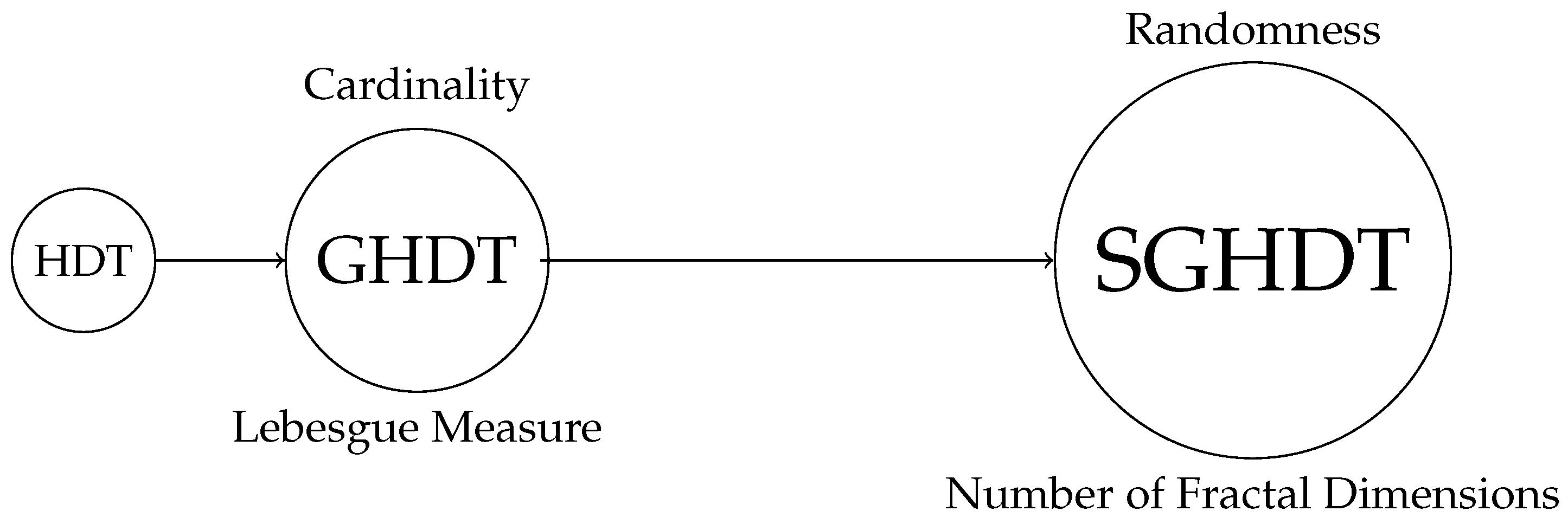
| HDT | For any real there is a continuum of [thin deterministic] fractals with Hausdorff dimension r in . |
| GHDT | For any real and there are aleph-two deterministic fractals with the Hausdorff dimension and Lebesgue measure l in . |
| SGHDT | For any real and there are aleph-two random fractals with the fractal dimension almost surely, and expected Lebesgue measure l in . Here, the fractal dimension is one of four dimensions: Hausdorff dimension, packing dimension, Assouad dimension, box dimension. |
5.2. Contributions
| Conclusion C1 | The cardinality of the set of all distinctive fractals in is invariant regardless of the used fractal dimension. |
| Conclusion C3 | The cardinality of the set of all distinctive fractals in is invariant regardless of their deterministic or random nature. |
5.3. Future Work
6. Conclusions
Funding
Institutional Review Board Statement
Informed Consent Statement
Data Availability Statement
Acknowledgments
Conflicts of Interest
Abbreviations
| a.s. | Almost Surely |
| FFP | Fat Fractal Perculation |
| HDT | Hausdorff Dimension Theorem |
| GCH | Generalized Continuum Hypothesis |
| GHDT | Generalized Hausdorff Dimension Theorem |
| MFP | Mandelbrot Fractal Perculation |
| SGHDT | Second Generalized Hausdorff Dimension Theorem |
References
- Mandelbrot, B.B. Renewal sets and random cutouts. Z. Wahrscheinlichkeitstheorie Und Verwandte Geb. 1972, 22, 145–157. [Google Scholar] [CrossRef]
- Mandelbrot, B.B. Intermittent turbulence in self-similar cascades: Divergence of high moments and dimension of the carrier. J. Fluid Mech. 1974, 62, 331–358. [Google Scholar] [CrossRef]
- Taylor, S.J. The measure theory of random fractals. Math. Proc. Camb. Philos. Soc. 1986, 100, 383–406. [Google Scholar] [CrossRef]
- Falconer, K.J. Random Fractals. Math. Proc. Camb. Phil. Soc. 1986, 100, 559–582. [Google Scholar] [CrossRef]
- Graf, S. Statistically self-similar fractals. Probab. Theory Relat. Fields 1987, 74, 357–392. [Google Scholar] [CrossRef]
- Frezza, M.; Bianchi, S.; Pianese, A. Fractal analysis of market (in)efficiency during the COVID-19. Financ. Res. Lett. 2021, 38. [Google Scholar] [CrossRef]
- Sivakumar, C. Stochastic evolution of the universe: A possible dynamical process leading to fractal structures. Pramana-J. Phys. 2018, 90. [Google Scholar] [CrossRef]
- Panigraphy, C.; Seal, A.; Mahato, N.K. Fractal dimension of synthesized and natural color images in lab spaces. Pattern Anal. Appl. 2020, 23, 819–836. [Google Scholar] [CrossRef]
- Frege, G. Foundations of Arithmetic; Austin, J.L., Translator; Oxford: Blackwell, UK, 1953. [Google Scholar]
- Brouwer, L.E.J. Over de Grondslagen der Wiskunde. Ph.D. Thesis, Universiteit van Amsterdam, Amsterdam, The Netherland, 1907. [Google Scholar]
- Waaldijk, F. On the Foundations of Constructive Mathematics–Especially in Relation to the Theory of Continuous Functions. Found. Sci. 2005, 10, 249–324. [Google Scholar] [CrossRef]
- Troelstra, A.S.; van Dalen, D. Constructivism in Mathematics: An Introduction (Two Volumes); Elsevier Science, Amsterdam: North Holland, The Netherland, 1988. [Google Scholar]
- Dowek, G. Chapter 8: Constructive Proofs and Algorithms. In Computation, Proof, Machine: Mathematics Enters a New Age; Guillot, P., Roman, M., Eds.; Cambridge University Press: Cambridge, UK, 2015. [Google Scholar]
- Klaus, M.; Schuster, P.; Schwichtenberg, H. (Eds.) Proof and Computation: Digitalization in Mathematics, Computer Science, and Philosophy; World Scientific: Hackensack, NJ, USA, 2018; pp. 1–46. [Google Scholar]
- Xiao, X.; Chen, H.; Bogdan, P. Deciphering the generating rules and functionalities of complex networks. Sci. Rep. 2021, 11, 22964. [Google Scholar] [CrossRef]
- Li, H. Fractal analysis of side channels for breakdown structures in XLPE cable insulation. J. Mater. Sci. Mater. Electron. 2013, 24, 1640–1643. [Google Scholar] [CrossRef]
- França, L.G.S.; Vivas Miranda, J.G.; Leite, M.; Sharma, N.K.; Walker, M.C.; Lemieux, L.; Wang, Y. Fractal and Multifractal Properties of Electrographic Recordings of Human Brain Activity: Toward Its Use as a Signal Feature for Machine Learning in Clinical Applications. Front. Physiol. 2018, 9, 1767. [Google Scholar] [CrossRef] [Green Version]
- Hu, S.; Cheng, Q.; Wang, L.; Xie, S. Multifractal characterization of urban residential land price in space and time. Appl. Geogr. 2012, 34, 161–170. [Google Scholar] [CrossRef]
- Brothers, H.J. Intervallic Scaling in the Bach Cello Suites. Fractals 2009, 17, 537–545. [Google Scholar] [CrossRef]
- Sharapov, S.; Sharapov, V. Dimensions of Some Generalized Cantor Sets. Available online: http://classes.yale.edu/fractals/FracAndDim/cantorDims/CantorDims.html (accessed on 3 April 2006).
- Soltanifar, M. On A Sequence of Cantor Fractals. Rose Hulman Undergrad. Math. J. 2006, 7, 1–9. [Google Scholar]
- Squillace, J. Estimating the fractal dimension of sets determined by nonergodic parameters. Discret. Contin. Dyn. Syst.-A 2017, 37, 5843–5859. [Google Scholar] [CrossRef] [Green Version]
- Gryszka, K. Hausdorff dimension is onto. Pr. Kola Mat. Uniw. Ped. W Krak 2019, 5, 13–22. [Google Scholar]
- Soltanifar, M. A Generalization of the Hausdorff Dimension Theorem for Deterministic Fractals. Mathematics 2021, 9, 1546. [Google Scholar] [CrossRef]
- Chen, C. A Class of Random Cantor Sets. Real Anal. Exch. 2017, 42, 79. [Google Scholar] [CrossRef]
- Chen, C. Distribution of random Cantor sets on tubes. Arkiv För Matematik 2016, 54, 39–54. [Google Scholar] [CrossRef]
- Mandelbrot, B.B. The Fractal Geometry of Nature; W. H. Freeman and Co.: San Francisco, CA, USA, 1982; ISBN 0-7167-1186-9. [Google Scholar]
- Falconer, K.J.; Grimmett, G.R. On the geometry of random cantor sets and fractal percolation. J. Theor. Probab. 1994, 7, 209–210. [Google Scholar] [CrossRef] [Green Version]
- Rosenthal, J.S. A First Look at Rigorous Probability Theory; World Scientific: Singapore, 2006; pp. 10, 21–22. [Google Scholar]
- Koivusalo, H. Dimension of Uniformly Random Self-Similar Fractals. Real Anal. Exch. 2014, 73, 10. [Google Scholar] [CrossRef]
- Broman, E.I.; Van De Brug, T.; Camia, F.; Joosten, M.; Meester, R. Fat fractal percolation and k-fractal percolation. ALEA Lat. Am. J. Probab. Math. Stat. 2012, 9, 279–301. [Google Scholar]
- Bishop, C.J. Fractals in Probability and Analysis, 1st ed.; Cambridge Studies in Advanced Mathematics, Series Number 162; Cambridge University Press: Cambridge, UK, 2017; pp. 105–107. [Google Scholar]
- Orzechowski, M.E. Percolation in Random Cantor Sets. Fractals 1997, 5, 101–109. [Google Scholar] [CrossRef]
- Tricot, C., Jr. Two definitions of fractional dimension. Math. Proc. Camb. Philos. Soc. 1982, 91, 57–74. [Google Scholar] [CrossRef]
- Assouad, P. Étude d’une dimension métrique liée à la possibilité de plongements dans Rn. Comptes Rendus de l’Académie des Sciences Série A-B 1979, 288, A731–A734. [Google Scholar]
- Bouligand, M.G. Ensembles impropres et nombredimensionnel. Bull. Des Sci. MathéMatiques 1928, 52, 320–344. [Google Scholar]
- Schroeder, M. Fractals, Chaos, Power Laws: Minutes from an Infinite Paradise; W. H. Freeman: New York, NY, USA, 1991; pp. 41–45. [Google Scholar]
- Schleicher, D. Hausdorff Dimension, Its Properties, and Its Surprises. Am. Math. Mon. 2007, 114, 509–528. [Google Scholar] [CrossRef] [Green Version]
- Bajnok, B. An Invitation to Abstract Mathematics, 2nd ed.; Springer: Berlin/Heidelberg, Germany, 2020; p. 325. [Google Scholar]
- Frederickson, F.; Kaplan, J.; Yorke, E.; Yorke, J. The Liapunov dimension of strange attractors. J. Differ. Equ. 1983, 49, 185–207. [Google Scholar] [CrossRef] [Green Version]
- Higuchi, T. Approach to an irregular time-series on the basis of the fractal theory. Phys. D 1988, 31, 277–283. [Google Scholar] [CrossRef]
- Peter, G. Generalized Dimensions of Strange Attractors. Phys. Lett. A 1983, 97, 227–230. [Google Scholar]
- Rényi, A. On the dimension and entropy of probability distributions. Acta Math. Acad. Sci. Hung. 1959, 10, 193–215. [Google Scholar] [CrossRef]
- Fernández-Martínez, M.; Sánchez-Granero, M. Fractal dimension for fractal structures. Topol. Its Appl. 2014, 163, 93–111. [Google Scholar] [CrossRef]

| E(λ(.)) | Constraints | |||
|---|---|---|---|---|
| 0 | ||||
| p | n |
Publisher’s Note: MDPI stays neutral with regard to jurisdictional claims in published maps and institutional affiliations. |
© 2022 by the author. Licensee MDPI, Basel, Switzerland. This article is an open access article distributed under the terms and conditions of the Creative Commons Attribution (CC BY) license (https://creativecommons.org/licenses/by/4.0/).
Share and Cite
Soltanifar, M. The Second Generalization of the Hausdorff Dimension Theorem for Random Fractals. Mathematics 2022, 10, 706. https://doi.org/10.3390/math10050706
Soltanifar M. The Second Generalization of the Hausdorff Dimension Theorem for Random Fractals. Mathematics. 2022; 10(5):706. https://doi.org/10.3390/math10050706
Chicago/Turabian StyleSoltanifar, Mohsen. 2022. "The Second Generalization of the Hausdorff Dimension Theorem for Random Fractals" Mathematics 10, no. 5: 706. https://doi.org/10.3390/math10050706
APA StyleSoltanifar, M. (2022). The Second Generalization of the Hausdorff Dimension Theorem for Random Fractals. Mathematics, 10(5), 706. https://doi.org/10.3390/math10050706