Deep-Processing Service and Pricing Decisions for Fresh Products with the Rate of Deterioration

Abstract

The mismatch between supply and demand for fresh products and those that can potentially lead to the risk of spoilage has posed huge losses for industrial companies. To reduce the risk of spoilage of fresh products, some firms have attempted to adopt a deep-processing service to alleviate the imbalance. Therefore, we developed a framework to control the spoilage of the product by taking into account the deep-processing service. First, a differential equation for an inventory model of fresh product and deep-processed product that depended on the selling price and the deteriorating rate was developed. Based on this, a profit model for fresh product and the deep-processed product was developed, and the condition of whether the deep-processing service was required was shown by optimization theory. Furthermore, the existence and its uniqueness of such proportion of deep processing and the selling price of the fresh product were proved. Research results showed the deep-processing service acted as a buffer against the mismatch between the supply and demand for the fresh product. Industrial companies should make lower profits but a quicker turnover by setting a lower selling price when both the deteriorating rate and initial freshness level are high, and vice versa.

1. Introduction

In the past 20 years, the demand for fresh products in China has grown tremendously. According to the Chinese government’s food consumption standards for 2020, the total demand for fresh products was projected to reach 420 million tons [1]. However, in 2017, the cold chain circulation rates of fruits and vegetables, meat, and seafood products in China were 26%, 39%, and 43%, respectively. The low level of cold chain logistics led to the pervasive paradox of a large production without a gold mine, and a bumper year without a bumper harvest [2]. For example, a litchi harvest in Zhanjiang, a city in China, did not lead to an increase in demand in 2018. In 2019, a high valuation led to pomegranates in Huili, the hometown of pomegranates in China, piling up on the ground and then spoiling.

Fresh products will lose their desirability as a result of spoilage if there is a large inventory at the end of the selling season. Furthermore, the maturity of fresh products is mostly concentrated in the summer and autumn, and the freshness period of many fresh products is relatively short, which leads to fresh products that are not suitable for long-distance transportation to reach the target market. Therefore, it is easy to suggest the fresh products be listed in regional clusters, which further aggravates the imbalance between supply and demand for the fresh products. In the face of fierce market competition, fruit farmers have to choose to sell fruits at a low price. In contrast, the prices of various processed fruits in supermarkets are quite high. For example, the market size of dried mangoes alone reached CNY 1 billion in China in 2019. Hence, it is necessary to extend the industrial chain and develop the product deep-processing industry to solve this problem, which could not only alleviate the imbalance between supply and demand in some places, but also improve the added value of fresh products and meet the different demands of consumers. A deep-processing service for fresh products can effectively avoid the risk of spoilage while also improving the added value of the agricultural product. Thus, a deep-processing service for fresh products not only effectively solves the problem of spoilage, but also solves the problem of the mismatch between the supply and demand for fresh agricultural products. The demand for fresh products depends on the selling price as well as the freshness, and thus the deep-processing service’s decisions, in turn, will influence the pricing decisions for the fresh products. In addition, the complexity of the structure of fresh products is exacerbated by its interaction with the deterioration rate. Under such settings, the deterioration rate will affect the inventory of the fresh product and deep-processed product. Consequently, the inventory affects the pricing decisions for the fresh product, and the pricing decisions will in turn pose a threat to the deep-processing service’s decisions.

Our aim was to explore a deep-processing service and how pricing decisions are made for fresh agricultural products while considering the deterioration rate. In particular, we were interested in researching the following in this work:

(1)

How the inventories of a fresh product and a deep-processed product were affected by the selling price and the deep-processing service;

(2)

How the deterioration rate affected the deep-processing service and the selling price of the fresh product;

(3)

How the selling price and the decisions of the deep-processing service affected the profit of the industrial company.

To address the questions as mentioned above, we chose an industrial company selling fresh product and deep-processed product as the research object. First, we developed a framework by taking into account the deep-processing service, and then inventory-decision models for fresh product and deep-processed product that depended on the selling price and the deteriorating rate of the fresh product were established. Furthermore, the profit model for fresh product and deep-processed product was developed.

Our study made two contributions to the field of deep-processing services and pricing decisions for fresh agricultural product.

First, specifically, we took a deep-processing service’s decisions into account in the existing framework of a fresh agricultural product from a novel perspective, which could control the spoilage of the fresh agricultural product. Considering the deterioration rate of the fresh product, the deep-processing service plays a role in alleviating the imbalance between the supply and demand for the fresh product, which will not only affect the pricing mechanisms of the industrial company, but also affect the sales strategies for fresh product. As a result, an industrial company should realize lower profits but a quicker turnover by setting a lower selling price when both the deteriorating rate and initial freshness level are high. Otherwise, an industrial company should set a higher selling price to sell fresh product in a rapid and profitable way.

Second, in this research framework, both fresh product and deep-processed product-inventory models were considered. The inventory decisions for fresh product will directly affect the inventory decisions for deep-processed products, and vice versa. Therefore, the pricing of fresh product further complicates their deep-processing and sales strategies.

The remainder of this paper is organized as follows. In next section, we provide a review of related literature. The problem formulation and assumptions are presented in Section 3. Section 4 presents the formulated mathematical models, including the fresh product inventory decision model, the deep-processing product inventory-decision model, and the industrial company profit model. Numerical results and sensitivity analyses are presented in Section 5, and in Section 6, we present conclusions regarding our findings and suggest possible future research. Technical proofs are relegated to Appendix A to smoothen the flow of our presentation.

2. Literature Review

Fresh agricultural products belong to the category of perishable products. Therefore, research on fresh agricultural products in operations management can refer to perishable products. Continuous deterioration is considered in most inventory studies of perishable products. Inventory of perishable products was first introduced by Ghare and Schrsder [3]. Based on this, subsequent research has been extensively pursued on the core factor of product demand. There are two types of demand for fresh products. One assumes that the demand is deterministic. The other assumes that demand is not fixed, but is affected by other factors or is random. A comprehensive survey of the earlier literature for deteriorating items is provided by Bakker et al. [4] and Janssen et al. [5], and we will not reiterate them here.

However, different from general perishable products with a fixed expiry date, consumers can perceive the freshness level of fresh agricultural products according to their appearance and smell, and take freshness as the external characterization of the quality of fresh agricultural products. Therefore, consumers are extremely susceptible to a change in the freshness level of fresh agricultural products. There is a lower demand as a result of a lower freshness level. At the same price, consumers will be more willing to buy the product with a high freshness level and good quality. There is an enormous amount of literature about preservation technology, or efforts to maintain freshness to keep the value of a product in order to increase the demand for a fresh agricultural product. In this course, Cai et al. [6] considered a fresh-product supply chain comprising a producer and a distributor, and derived the optimal inventory level, the level of freshness-maintaining efforts, and the selling price of the distributor. A comprehensive survey can be found in Shukla et al. [7]. Cai et al. [8] analyzed the optimal policies for three supply chain members in a fresh-product supply chain, including the order quantity and retail price of the distributor, the third-party logistic provider’s transportation fee, and the producer’s shipping quantity and wholesale price. From this, Chen et al. [9] analyzed the optimal ordering and pricing policies of perishable products with random and partial quality deterioration during long-distance transportation. Cai and Zhou [10] extended the previous research to the optimal order quantity and the level of freshness-maintaining efforts of the producer when the demand changed abruptly. Afterward, Liu et al. [11] studied the influence mechanism of information sharing on preservation efforts and pricing in a supply chain in which the producer was required to decide the optimal level of freshness-maintaining effort, and the online retailer provided value-added services. Liu and Chen [12] expanded the model from a single-stage decision to a multistage decision on this basis. The above literature mainly focused on the decisions regarding the freshness-maintaining efforts, while Zanoni and Zavanella [13] considered specific preservation technology and obtained the conditions for refrigerating or freezing food and the corresponding inventory strategies. Yu and Xiao [14] also analyzed the optimal cold chain service level and pricing policies for a seasonal perishable with a rate of deterioration that could be controlled by preservation technology. Pan et al. [15] further enriched the inventory model by considering uncertain logistics, while Yu et al. [16] considered the case of a fresh agricultural product supply chain with multiple competing retailers. In contrast, He et al. [17] presented an online presale model of fresh produce from a competitive perspective, and further established a deterioration inventory model to obtain the optimal market entry strategy of online presales. Ma et al. [18] investigated the optimal level of freshness-maintaining efforts under the constraints of carbon trading in a three-stage cold chain. They coordinated this with a revenue cost-sharing contract. Yan et al. [19] studied the impact of consumer behaviors on supply chain decision making for fresh agricultural products. Song et al. [20] derived the optimal pricing and channel selection decisions for a perishable product distributed through multiple channels. Chernonog et al. [21] considered the optimal marketing policy for a perishable product in a two-stage supply chain.

The above literature on perishable product inventory focused on the demand for a perishable product. For fresh agricultural products with perceived freshness, the freshness level is introduced to establish an inventory model in which the demand for a fresh agricultural product depends on its price and freshness. In addition, a fresh agricultural product combines the two natures of value loss and physical loss. The former refers to a loss caused by external factors such as temperature and humidity in the environment where the product is located, which reduces the quality and freshness of the product over time. The latter refers to complete corruption or loss of utility of some commodities caused by the deterioration rate. Therefore, the deterioration rate was also a focus of research on perishable product inventory management. In addition to the above research assuming that the deterioration rate was constant, some research also studied a nonconstant deterioration rate. For example, Singh et al. [22] established the EOQ model for perishable products whose deterioration rate is a three-parameter Weibull distribution under the condition of time-dependent demand. Another stream of related research concerned inventory control, and mainly focused on the demand for a fresh agricultural product, delivery time, payment terms, and preservation-technology investment. For example, Chen et al. [23] considered the effects of both inventory and selling price on demand, and in this respect scheduled an inventory model for deteriorating items to discuss the optimal pricing and replenishment decisions. Chung et al. [24] provided an inventory model for deteriorating items with cash discounts and trade credits, and then derived the optimal solutions for the total cost. Since fresh agricultural products involve deterioration, they also involve the issue of shelf life. Wu et al. [25] established an inventory model for perishable products with expiration dates, and they derived the retailer’s optimal lot-sizing policies. From this, Wu et al. [26] studied a retailer’s optimal credit period for a fresh agricultural product with an expiration date. Alternatively, Wu et al. [27] analyzed the pricing policy for a perishable product with an expiration date. Duan and Liao et al. [28] investigated perishable supply chain inventory optimization based on updating of demand information. Li et al. [29] analyzed the pricing and replenishment decisions for deteriorating items with preservation technology investment. Based on this, Mashud et al. [30] studied the optimal level of freshness-maintaining efforts and pricing policies for a fresh agricultural product while considering controllable carbon emissions. Similarly, Sepehri et al. [31] proposed an inventory system for perishable items under the permissible delay in payments by adding carbon-emission regulations into the inventory model. Jani et al. [32] analyzed a preservation technology investment policy for perishable products with a maximum lifetime with trade credits and the supposition of variable demand. Hatami-Marbinia et al. [33] investigated the optimal inventory-control strategy for perishable goods from the perspective of production planning of a network by using a combination of a simulated annealing algorithm and the Taguchi experimental design approach. Mohammadi [34] developed a waste-reduction approach to a fresh agricultural product by considering the quantity and quality deterioration. The relevant research assumed that the deterioration rate was fixed. For instance, Chen et al. [35] proposed optimal ordering and pricing strategies for fresh products with different perishabilities, and provided sales strategies for high- and low-quality products.

Research on perishable products in the operations-management literature has focused on pricing, ordering, preservation, and channel selection without considering the deep-processing service of fresh agricultural products. The deep-processing service not only affects the pricing of fresh agricultural products, but also acts as a buffer to reduce the uncertainty of the demand for fresh agricultural products, and in turn further influences the pricing of fresh agricultural products. Therefore, from the perspective of a deep-processing service for fresh agricultural products, this study introduced a deep-processing service into a pricing-decision model, and explored the influence mechanism of the deep-processing service on a fresh agricultural product.

3. Problem Definition and Assumptions

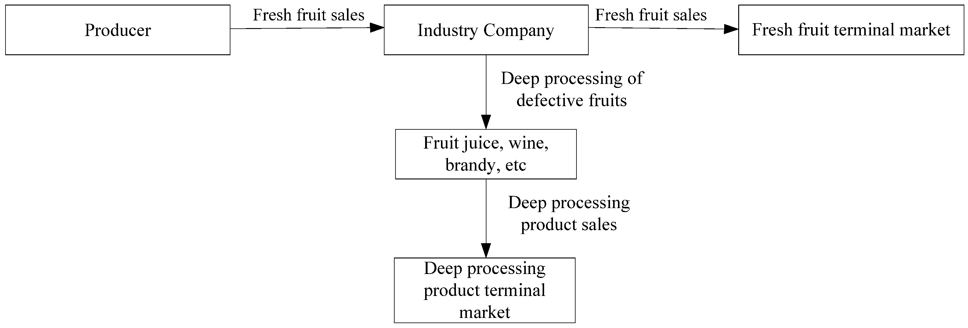
Zhongxin Industrial Company (hereinafter referred to as the producer) is responsible for planting kiwifruit according to uniform standards, and its annual output of kiwifruit is $Q$. The fresh kiwifruit produced by the upstream producer is purchased by Liupanshui Liangdu Kiwifruit Industry Co., Ltd. (hereinafter referred to as the industrial company) at a purchase price of $w$. The purchase price is based on the comprehensive consideration of management cost, annual output, and primary market conditions. After purchasing, the industrial company mainly sells fresh kiwifruit (hereinafter referred to as fresh product; the proportion of fresh product sales is about 80%), and carries out a deep-processing service on some defective products and products that cannot be sold at the end of selling season, which are mainly processed into fruit juice, fruit wine, brandy, etc. The specific process is shown in Figure 1.

The demand for fresh product depends on its selling price and freshness level, $D_1\left(p_1,\theta \left(t\right)\right)=d\left(p_1\right){\theta }_0^t$, where $d\left(p_1\right)=\left(a_1-b_1{p}_1\right)$. In addition, because the kiwifruit can only be grown locally due to special geological conditions (its variety is red kiwifruit), the industrial company can set the market selling price as $p_1$ with reference to the price of Zespri kiwifruit in New Zealand. The fresh product is generally sold after being picked in early August. A function $\theta \left(t\right)={\theta }_0^t$, defined over $\left[0,1\right]$ as the freshness level of fresh product at time $t$, which declines with time. $t=0$ is the time at which fresh product arrives at the warehouse of the industrial company, and ${\theta }_0$ is the initial freshness level of fresh product at $t=0$, ${\theta }_0\le 1$. Due to the decline in freshness and deterioration during the sales process, the industrial company generally needs to decide the deep-processed proportion $\gamma$ in mid-September ($t_d$) according to the previous sales, and the deep-processing cost per unit is $c$. Since there is a one-to-one correspondence between the unit quantity $q$ of fresh product and the final quantity $g\left(q\right)$ of deep-processed product, to simplify the calculation, let $g\left(q\right)=q$. The demand for deep-processed product depends only on its selling price; that is, $D_2\left(p_2\right)=d\left(p_2\right)$, where $d\left(p_2\right)=\left(a_2-b_2{p}_2\right)$. Since fruit juice, fruit wine, and brandy are in a perfectly competitive market, the selling price $p_2$ of the deep-processed products is determined by the market.

The following notations were used to model our problem. For ease of reference, we list the notations we used in this paper in

Table 1. List of notation.

Symbol	Description
$Q$	Purchase quantity of the industrial company (units)
$w$	Purchase price per unit (CNY/unit)
$p_1$$,p_2$	Selling price per unit of fresh product and deep-processed product (CNY/unit)
$c$	Fresh product deep-processing cost per unit (CNY/unit)
$h$	Holding cost per unit per unit time (CNY/unit/unit time)
$\lambda$	$\mathrm{Deterioration}\mathrm{rate}\mathrm{of}\mathrm{fresh}\mathrm{product},0\le \lambda \le 1$
$t_d$	Time from which deep processing of fresh product starts (time)
${\theta }_0$	Initial freshness level of fresh product
$\theta (t)$	$\mathrm{Freshness}\mathrm{level}\mathrm{of}\mathrm{fresh}\mathrm{product}\mathrm{at}\mathrm{time}t$
$D_1$$,D_2$	Demand for fresh product and deep-processed product (units)
$a_1$$,a_2$	Market scale of fresh product and deep-processed products
$b_1$$,b_2$	Price-sensitive factors of fresh product and deep-processed products
$\gamma$	$\mathrm{Proportion}\mathrm{of}\mathrm{deep}-\mathrm{processed}\mathrm{fresh}\mathrm{product},0\le \gamma \le 1$
$I_1(t)$$,I_2(t)$	$\mathrm{Inventory}\mathrm{level}\mathrm{of}\mathrm{fresh}\mathrm{product}\mathrm{and}\mathrm{deep}-\mathrm{processed}\mathrm{product}\mathrm{at}\mathrm{time}t$ (units)
$\pi$	Total profit of the industrial company (CNY)

.

4. Model Formulation and Analysis

In the early product sales, within $\left[0,t_d\right]$, the industrial company directly sells fresh product to retailers. In order to avoid the risk of unsalable and rotten products, the industrial company will carry out deep processing of part of its unsold fresh product at time $t_d$. We assumed that the processing proportion was $\gamma$, and the remaining fresh product was directly sold as fresh product. The time when the industrial company began deep processing of fresh product is $t_d$, and the time when the fresh product inventory level drops to 0 is $T_1$. Based on values of $t_d$ and $T_1$, there are two cases: $0\le T_1\le t_d$ and $0\le t_d<T_1$. For these two cases, we developed the inventory model and the industrial company profit model accordingly.

4.1. Inventory Model of Fresh Product

The inventory of fresh product is $Q$ units at $t=0$, and then gradually drops to 0 at $t=T_1$ due to the combination effects of demand and deterioration. Thus, this study referred to the perishable inventory model of Dye et al. [36], and the differential equation for the inventory level during the period is:

$$\begin{array}{cc}\frac{d{I}_1\left(t\right)}{dt}=-\lambda I_1\left(t\right)-d\left(p_1\right){\theta }_0^t& 0\le t\le T_1\end{array}$$

(1)

We divided the time interval $\left[0,T_1\right]$ into two stages: $\left[0,t_d\right]$ and $\left[t_d,T_1\right]$. Let the inventory at time t during $\left[0,t_d\right]$ and $\left[t_d,T_1\right]$ be $I_1^1\left(t\right)$ and $I_1^2\left(t\right)$, respectively. With boundary conditions $I_1^1\left(0\right)=Q$ and $I_1^2\left(t_d\right)=\left(1-\gamma \right)\left(Q{e}^{-\lambda t_d}+\frac{d\left(p_1\right)\left(e^{-\lambda t_d}-{\theta }_0^{t_d}\right)}{\ln {\theta }_0+\lambda }\right)$, solving Equation (1) yields:

$$I_1\left(t\right)=\{\begin{array}{cc}{I}_1^1\left(t\right)=Q{e}^{-\lambda t}+\frac{d\left(p_1\right)\left(e^{-\lambda t}-{\theta }_0^t\right)}{\ln {\theta }_0+\lambda }& 0\le t\le t_d\\ I_1^2(t)=\frac{-d\left(p_1\right){\theta }_0^t}{\ln {\theta }_0+\lambda }+\left(1-\gamma \right)I_1^1\left(t_d\right)e^{\lambda \left(t_d-t\right)}+\frac{d\left(p_1\right){\theta }_0^{t_d}{e}^{\lambda \left(t_d-t\right)}}{\ln {\theta }_0+\lambda }& t_d\le t\le T_1\end{array}$$

(2)

Proposition 1.

The fresh product inventory level $I_1\left(t\right)$is a decreasing function of the initial freshness level ${\theta }_0$.

Proof of Proposition 1.

Taking the first-order partial derivative of $I_1^1\left(t\right)$ with respect to ${\theta }_0$, we get $\frac{\partial I_1^1\left(t\right)}{\partial {\theta }_0}=\frac{d\left(p_1\right)\left[-t{\theta }_0^t\left(\ln {\theta }_0+\lambda \right)-e^{-\lambda t}+{\theta }_0^t\right]}{{\left(\ln {\theta }_0+\lambda \right)}^2\theta }$. When $\lambda >-\ln {\theta }_0$ holds, we can easily prove $\frac{\partial \left[-t{\theta }_0^t\left(\ln {\theta }_0+\lambda \right)-e^{-\lambda t}+{\theta }_0^t\right]}{\partial \lambda }=-t{\theta }_0^t+t{e}^{-\lambda t}<0$, and $\left[-t{\theta }_0^t\left(\ln {\theta }_0+\lambda \right)-e^{-\lambda t}+{\theta }_0^t\right]<\left[-t{\theta }_0^t\left(\ln {\theta }_0+\lambda \right)-e^{-\lambda t}+{\theta }_0^t\right]|\left(\lambda =-\ln {\theta }_0\right)=0$. Similarly, if $\lambda <-\ln {\theta }_0$, we have $\frac{\partial \left[-t{\theta }_0^t\left(\ln {\theta }_0+\lambda \right)-e^{-\lambda t}+{\theta }_0^t\right]}{\partial \lambda }=-t{\theta }_0^t+t{e}^{-\lambda t}>0$, and $\left[-t{\theta }_0^t\left(\ln {\theta }_0+\lambda \right)-e^{-\lambda t}+{\theta }_0^t\right]<\left[-t{\theta }_0^t\left(\ln {\theta }_0+\lambda \right)-e^{-\lambda t}+{\theta }_0^t\right]|\left(\lambda =-\ln {\theta }_0\right)=0$. Therefore, we can easily prove that $\frac{\partial I_1^1\left(t\right)}{\partial {\theta }_0}=\frac{d\left(p_1\right)\left[-t{\theta }_0^t\left(\ln {\theta }_0+\lambda \right)-e^{-\lambda t}+{\theta }_0^t\right]}{{\left(\ln {\theta }_0+\lambda \right)}^2{\theta }_0}<0$. Similarly, $\begin{array}{l}\frac{\partial I_1^2\left(t\right)}{\partial {\theta }_0}=\\ \frac{d\left(p_1\right)\left\{\left(1-\gamma \right)\left[-t{\theta }_0^t\left(\ln {\theta }_0+\lambda \right)-e^{-\lambda t}+{\theta }_0^t\right]e^{\lambda \left(t_d-t\right)}+\left[\left(t_d{\theta }_0^{t_d}{e}^{\lambda \left(t_d-t\right)}-t{\theta }_0^t\right)\left(\ln {\theta }_0+\lambda \right)-{\theta }_0^{t_d}{e}^{\lambda \left(t_d-t\right)}+{\theta }_0^t\right]\right\}}{{\left(\ln {\theta }_0+\lambda \right)}^2\theta }<0\end{array}$. Thus, the fresh product inventory level decreases as the initial freshness level ${\theta }_0$ increases. □

Proposition 1 demonstrates that the inventory level of fresh product will decrease with an increase in the initial freshness level, because the higher the freshness level of the fresh product, the better its flavor and nutritional quality, and the further the expiry date. Under the same conditions, the higher the freshness level of the fresh product, the greater the purchase quantity of retailers, and the faster the inventory of the industrial company will decline. Therefore, the industrial company tends to require the producer to provide fresh product with a higher freshness level in order to reduce the inventory loss due to deterioration and speed up the inventory turnover.

In addition, Formula (2) demonstrates that when the fresh product market is popular, the inventory of the industrial company will decrease rapidly; that is, all fresh product will be sold. Therefore, the industrial company does not need to consider the deep processing of fresh product when the processing time of fresh product satisfies the time $0\le T_1\le t_d$. Otherwise, it is necessary to decide the proportion of fresh product for deep processing when the processing time satisfies the time $0\le t_d<T_1$. In summary, the proposition below characterizes the time when the inventory of fresh product drops to 0.

Proposition 2.

The time when the inventory of fresh product drops to 0 satisfies

$$T_1=\{\begin{array}{cc}\frac{\ln \left(\frac{Q\left(\ln {\theta }_0+\lambda \right)}{d\left(p_1\right)}+1\right)}{\ln \theta +\lambda }& d(p_1)\ge \frac{Q{e}^{-\lambda t_d}\left(\ln {\theta }_0+\lambda \right)}{{\theta }_0^{t_d}-e^{-\lambda t_d}}\\ \frac{\ln \left[\frac{\left(\ln {\theta }_0+\lambda \right)\left(1-\gamma \right)I_1^1\left(t_d\right)}{d\left(p_1\right)}+{\theta }_0^{t_d}\right]+\lambda t_d}{\ln {\theta }_0+\lambda }& 0\le d\left(p_1\right)<\frac{Q{e}^{-\lambda t_d}\left(\ln {\theta }_0+\lambda \right)}{{\theta }_0^{t_d}-e^{-\lambda t_d}}\end{array}$$

Proof of Proposition 2.

When the processing time of fresh product satisfies $0\le T_1\le t_d$, it means that the fresh product inventory has dropped to 0 before time $t_d$, and all the products are sold in the form of fresh product. We can easily prove that $d(p_1)\ge \frac{Q{e}^{-\lambda t_d}\left(\ln {\theta }_0+\lambda \right)}{{\theta }_0^{t_d}-e^{-\lambda t_d}}$ holds when $I_1^1\left(t_d\right)\le 0$ holds. Let $I_1^1\left(T_1\right)=0$ in Formula (2), and the time when the fresh product inventory drops to 0 can be obtained, as shown in Formula (3):

$$T_1=\frac{\ln \left(\frac{Q\left(\ln {\theta }_0+\lambda \right)}{d\left(p_1\right)}+1\right)}{\ln {\theta }_0+\lambda }$$

(3)

When the processing time of fresh product satisfies $0\le t_d<T_1$, the industrial company processes the unsold fresh product at time $t_d$, at which time the fresh product inventory $I_1^1\left(t_d\right)>0$ and $0\le d\left(p_1\right)<\frac{Q{e}^{-\lambda t_d}\left(\ln {\theta }_0+\lambda \right)}{{\theta }_0^{t_d}-e^{-\lambda t_d}}$ are obtained. Let $I_1^2\left(T_1\right)=0$; from Formula (2), we can obtain the time when the fresh product inventory drops to 0, as shown in Formula (4):

$$T_1=\frac{\ln \left[\frac{\left(\ln {\theta }_0+\lambda \right)\left(1-\gamma \right)I_1^1\left(t_d\right)}{d\left(p_1\right)}+{\theta }_0^{t_d}\right]+\lambda t_d}{\ln {\theta }_0+\lambda }$$

(4)

Proposition 2 indicates that when the demand for fresh product is high, the inventory of fresh product will decline rapidly. The industrial company sells all the fresh product with a higher freshness level before time $t_d$. Hence, there is no need to make the decision to deep process. The inventory turnover of fresh product is slow when the fresh product market is dampened. In order to reduce the risk of spoilage, the industrial company should implement the deep processing using a proportion of the fresh product. □

4.2. Inventory Model Deep-Processed Product

The freshness level of the fresh product continues to decline with time, which results in a lower demand. The industrial company will control the spoilage of the product by processing part of the unsold fresh product at time $t_d$ in the case of $I_1^1\left(t_d\right)>0$. The inventory of the deep-processed product at time t over $\left[t_d,T_2\right]$ can be described by the following equation:

$$\frac{d{I}_2\left(t\right)}{dt}=-d\left(p_2\right)$$

(5)

We can solve the differential Equation (5) with the boundary condition $I_2\left(t_d\right)=\gamma I_1^1\left(t_{{}_d}\right)$. Let $I_2\left(t\right)$ be the solution to Equation (5):

$$I_2\left(t\right)=d\left(p_2\right)\left(t_d-t\right)+\gamma I_1^1\left(t_d\right)t_d\le t\le T_2$$

(6)

Proposition 3.

The time when the deep-processed product inventory level drops to 0 satisfies

$$T_2=\frac{\gamma I_1^1\left(t_d\right)}{d\left(p_2\right)}+t_d$$

(7)

Proof of Proposition 3.

Similar to the proof process of Proposition 2, let $I_2\left(T_2\right)=0$, which can be proved by Formula (6). □

Proposition 3 indicates that the time when the inventory of deep-processed products drops to 0 consists of $t_d$ and the sale time of the deep-processed product. Although the time of deep processing $t_d$ is predetermined, there is a great correlation between the sale time of fresh product and the time of deep processing. There needs to be more time to sell out of processing product if the deep-processing time is earlier, because there are higher inventories of fresh product and deep-processed product, and vice versa.

The above research focused on the inventory model of fresh product and the deep-processed product. The industrial company further affects the inventory of the two by pricing and determining the proportion of deep processing, which in turn affects the sale time. Therefore, we will further determine the optimal pricing and deep-processed proportion from the perspective of industrial company profit in the next subsection.

4.3. Profit Model of the Industrial Company

According to the above analysis, we will further discuss the profit of the industrial company in two cases. First, when the fresh product market is popular, the condition $d(p_1)\ge \left(Q{e}^{-\lambda t_d}\left(\ln \theta +\lambda \right)\right)/\left({\theta }^{t_d}-e^{-\lambda t_d}\right)$ is satisfied. In this case, the industrial company’s objective at this stage is to maximize its profit by setting an optimal selling price. The profit is defined by Formula (8):

$${\pi }_1\left(p_1\right)=p_1\left(Q-\lambda {\displaystyle {\int }_0^{T_1}{I}_1^1\left(t\right)dt}\right)-h{\displaystyle {\int }_0^{T_1}{I}_1^1\left(t\right)dt}-wQ$$

(8)

Formula (8) can be interpreted as follows: the first term represents the revenue from sales of fresh product. The second and third terms represent the costs of leftover inventory and purchases, respectively.

When the fresh product market is dampened; that is, when the demand satisfies $d(p_1)<\left(Q{e}^{-\lambda t_d}\left(\ln \theta +\lambda \right)\right)/\left({\theta }^{t_d}-e^{-\lambda t_d}\right)$, the industrial company not only needs to sell fresh product, but also needs to consider using the deep-processing service and sell deep-processed product. In this case, the profit of the industrial company includes the sales revenue from fresh product and deep-processed product. The industrial company’s objective at this stage is to maximize its expected profit by setting an optimal selling price and proportion of deep-processed fresh product. The profit is defined by Formula (9):

$${\pi }_2\left(p_1,\gamma \right)=R-HC-PC-OC$$

(9)

Formula (9) can be interpreted as follows: the first term represents the revenue from sales of fresh product and deep-processed product. The second, third, and fourth terms represent the cost of leftover inventory, deep-processed product, and purchases, respectively. $R$, $HC$, $PC$, and $OC$ are defined by:

$$\begin{gathered} R=p_1[Q-\gamma I_1^1\left(t_d\right)-\lambda {\displaystyle {\int }_0^{t_d}{I}_1^1\left(t\right)dt}-\lambda {\displaystyle {\int }_{t_d}^{T_1}{I}_1^2\left(t\right)dt}]+p_2\gamma I_1^1\left(t_d\right), \\ HC=h\left({\displaystyle {\int }_0^{t_d}{I}_1^1(t)dt+{\displaystyle {\int }_{t_d}^{T_1}{I}_1^2(t)dt}}+{\displaystyle {\int }_{t_d}^{T_2}{I}_2(t)dt}\right),PC=c\gamma I_1^1(t_d), \end{gathered}$$

and $OC=wQ$.

Based on the above two cases, the profit function of the industrial company is given by Formula (10):

$$\pi =\{\begin{array}{cc}{\pi }_1\left(p_1\right)& 0\le p_1\le \frac{a_1}{b_1}-\frac{Q{e}^{-\lambda t_d}\left(\ln {\theta }_0+\lambda \right)}{b_1\left({\theta }_0^{t_d}-e^{-\lambda t_d}\right)}\\ {\pi }_2\left(p_1,\gamma \right)& \frac{a_1}{b_1}-\frac{Q{e}^{-\lambda t_d}\left(\ln {\theta }_0+\lambda \right)}{b_1\left({\theta }_0^{t_d}-e^{-\lambda t_d}\right)}<p_1\le \frac{a_1}{b_1}\end{array}$$

(10)

Since $\underset{p_1\to A}{\lim }{\pi }_2\left(p_1,\gamma \right)={\pi }_2\left(A\right)=\left[p_1\left(Q-\lambda {\displaystyle {\int }_0^{t_d}{I}_1^1\left(t\right)dt}\right)-h{\displaystyle {\int }_0^{t_d}{I}_1^1\left(t\right)dt}-wQ\right]|\left(p_1=A\right)$, where $A$ is defined by $A=\frac{a_1}{b_1}-\frac{Q{e}^{-\lambda t_d}\left(\ln {\theta }_0+\lambda \right)}{b_1\left({\theta }_0^{t_d}-e^{-\lambda t_d}\right)}$, then $\pi$ is a continuous function in the field of definition. Since the decision variables are $\gamma$ and $p_1$, it is necessary to obtain the optimal value of the decision variable by maximizing the profit of the industrial company. We next identify some conditions under which the existence and uniqueness of the solution can be guaranteed.

Proposition 4.

If $0\le p_1\le \frac{a_1}{b_1}-\frac{Q{e}^{-\lambda t_d}\left(\ln {\theta }_0+\lambda \right)}{b_1\left({\theta }_0^{t_d}-e^{-\lambda t_d}\right)}$, then ${\pi }_1\left(p_1\right)$is a concave function of the selling price$p_1$; that is, there exists a unique$p_1{}^{\ast }$that maximizes${\pi }_1\left(p_1\right)$. If$\frac{a_1}{b_1}-\frac{Q{e}^{-\lambda t_d}\left(\ln {\theta }_0+\lambda \right)}{b_1\left({\theta }_0^{t_d}-e^{-\lambda t_d}\right)}<p_1\le \frac{a_1}{b_1}$and$0\le \frac{d\left(p_2\right)}{h}\le \frac{2b_1\left[\ln \theta \left(e^{-\lambda t_d}-1\right)\left({\theta }_0^{t_d}-1\right)+2\lambda \left({\theta }_0^{t_d}-1\right)\right]}{\ln {\theta }_0\left(\ln {\theta }_0+\lambda \right)}$, then there exists a unique${\gamma }^{\ast }$and$p_1^{\ast }$that maximize${\pi }_2\left(p_1,\gamma \right)$.

Proof of Proposition 4. See Appendix A. □

Proposition 4 shows that deep processing acts as a buffer against the imbalance between the supply and demand for the fresh product by controlling the spoilage of the product. When the deterioration rate and the initial freshness level are higher, the industrial company should set a lower selling price in order to sell the fresh product quickly, realizing lower profits but a quicker turnover. When the deterioration rate and initial freshness level are lower and the price of the deep-processed product is high, the industrial company will set a higher selling price in order to sell fresh product and deep-processed product in a profitable way. It can be obtained that $e^{-\lambda t_d}\left(\ln {\theta }_0+\lambda \right)/\left({\theta }_0^{t_d}-e^{-\lambda t_d}\right)$ is a decreasing function of the deterioration rate and initial freshness level. Therefore, as the deterioration rate increases, there is more room for the industrial company to set a lower selling price, and vice versa. When the deterioration rate and the initial freshness level are higher, the freshness of fresh product is high when it is newly launched, and the industrial company can quickly increase the sales volume by setting a lower selling price. Although the deterioration rate is higher, the loss of fresh product is not larger due to the quicker turnover, and its profit will be higher. When the deterioration rate and initial freshness level are lower and the price of the deep-processed product is higher, the quality of the fresh product on the market is not good. In order to make up for the loss, the industrial company mainly relies on the sales of deep-processed product to increase its profit. Consequently, on the one hand, a higher selling price will improve the profit of fresh product as a result of the lower deterioration rate; while on the other hand, a higher selling price can slow down the sale of fresh product, which increases the profitability of the deep-processed product. Therefore, the industrial company can reap the total revenue of the two stages by setting a higher selling price for fresh product.

5. Numerical Example and Sensitivity Analysis

In this section, we report the results of our computational studies, which contain a numerical example in order to demonstrate the applicability of the proposed model, and were conducted to investigate the impacts of the key parameters on the optimal deep-processing service, pricing decisions, and profits of the industrial company. Throughout these computational studies, the nominal values for the input parameters were $Q=4500$ units, $w=3$ $, $c=1$ $, $h=0.2$ $, $t_d=6$ months, $a_1=910$, $b_1=60$, $a_2=216$, $b_2=10$, $p_2=21$ $, $\lambda =0.12$, and ${\theta }_0=0.94$. We used an algorithm to find the optimal values of $p_1$, $\gamma$, and $\pi$.

Step 1:	$\mathrm{Input}\mathrm{the}\mathrm{values}\mathrm{of}\mathrm{parameters}.\mathrm{If}\mathrm{input}\mathrm{parameters}\mathrm{not}\mathrm{in}\mathrm{the}\mathrm{range}\mathrm{of}\mathrm{Formula}\left(\mathrm{A}10\right)\mathrm{and}A>0$, the solution is infeasible.
Step 2:	$\mathrm{Set}\frac{\partial {\pi }_1\left(p_1\right)}{\partial p_1}=0$$,\mathrm{and}\mathrm{find}\mathrm{the}\mathrm{optimal}\mathrm{variables}{p}_1^1{}^{\ast }$$.\mathrm{In}\mathrm{this}\mathrm{step},\mathrm{the}\mathrm{optimal}\mathrm{variable}{\gamma }_1^{\ast }$ is equal to 0.
Step 3:	$\mathrm{Substitute}\mathrm{the}\mathrm{optimal}\mathrm{variables}\mathrm{obtained}\mathrm{into}\mathrm{the}\mathrm{profit}\mathrm{Formula}\left(8\right)\mathrm{and}\mathrm{find}\mathrm{the}\mathrm{optimal}\mathrm{total}\mathrm{profit}{\pi }_1\left(p_1^1{}^{\ast }\right)$.
Step 4:	$\mathrm{Set}\frac{\partial {\pi }_2\left(p_1,{\gamma }^{\ast }(p_1)\right)}{\partial p_1{}^{\ast }}=0$$,\mathrm{and}\mathrm{calculate}{p}_1^2{}^{\ast }$$\mathrm{and}{\gamma }_2^{\ast }$ using Formula (A5).
Step 5:	$\mathrm{Substitute}\mathrm{the}\mathrm{optimal}\mathrm{variables}\mathrm{obtained}\mathrm{into}\mathrm{the}\mathrm{profit}\mathrm{Formula}\left(9\right)\mathrm{and}\mathrm{find}\mathrm{the}\mathrm{optimal}\mathrm{total}\mathrm{profit}{\pi }_2\left(p_1^2{}^{\ast },{\gamma }_2^{\ast }\right)$.
Step 6:	$\mathrm{Compare}\mathrm{the}\mathrm{values}\mathrm{of}{\pi }_1\left(p_1^1{}^{\ast }\right)$$\mathrm{and}{\pi }_2\left(p_1^2{}^{\ast },{\gamma }_2^{\ast }\right)$$.\mathrm{If}{\pi }_1\left(p_1^1{}^{\ast }\right)\ge {\pi }_2\left(p_1^2{}^{\ast },{\gamma }_2^{\ast }\right)$$,\mathrm{then}\mathrm{the}\mathrm{optimal}\mathrm{values}\mathrm{of}\mathrm{decision}\mathrm{variables}\mathrm{are}{p}_1^{\ast }=p_1^1{}^{\ast }$$,{\gamma }^{\ast }={\gamma }_1^{\ast }$$,\mathrm{and}\mathrm{the}\mathrm{total}\mathrm{profit}\mathrm{is}{\pi }^{\ast }={\pi }_1\left(p_1^1{}^{\ast }\right)$$;\mathrm{otherwise}\mathrm{the}\mathrm{optimal}\mathrm{values}\mathrm{are}{p}_1^{\ast }=p_1^2{}^{\ast }$$,{\gamma }^{\ast }={\gamma }_2^{\ast }$$,\mathrm{and}{\pi }^{\ast }={\pi }_2\left(p_1^2{}^{\ast },{\gamma }_2^{\ast }\right)$.
Step 7:	Stop.

Using the above solution procedure, the results from the algorithm presented were $p_1^{\ast }=10.15$ $, ${\gamma }^{\ast }=0.36$, ${\pi }^{\ast }=10018.40$ $.

For the example above, the plot of $\pi$ against $p_1$ and $\gamma$ is presented in Figure 2, the plot of $I_1^1\left(t_d\right)$ against $p_1$ and $\gamma$ is presented in Figure 3, and the plot of $I_2\left(t_d\right)$ against $p_1$ and $\gamma$ is presented in Figure 4.

The effects of the change in the values of the selling price $p_1$ and the deep-processed proportion $\gamma$ on the total profit $\pi$, as well as on the inventories of fresh product and deep-processed product at $t=t_d$, are presented in Figure 2, Figure 3 and Figure 4. From Figure 3, we can find that when $p_1$ is small, the $I_1^1\left(t_d\right)$ and $I_2\left(t_d\right)$ are zero. This is because when $0\le p_1\le \frac{a_1}{b_1}-\frac{Q{e}^{-\lambda t_d}\left(\ln {\theta }_0+\lambda \right)}{b_1\left({\theta }_0^{t_d}-e^{-\lambda t_d}\right)}$; that is, $d(p_1)\ge \left(Q{e}^{-\lambda t_d}\left(\ln \theta +\lambda \right)\right)/\left({\theta }^{t_d}-e^{-\lambda t_d}\right)$, the fresh product inventory has dropped rapidly to 0 before time $t_d$, and all the products are sold in the form of fresh product. When $p_1$ is large, $I_1^1\left(t_d\right)>0$, thus, the industrial company not only needs to sell fresh product, but also needs to consider the deep-processing service and sell deep-processed product. We can see from Figure 4 that $I_2\left(t_d\right)$ is affected by $p_1$ and $\gamma$; that is, $I_2\left(t_d\right)$ increases with the increases in $p_1$ and $\gamma$, which will further influence the profit of the deep-processed product and the total profit $\pi$ (see Figure 2). As a result, the pricing of fresh product will directly influence the demand for and the inventory level of fresh product, which will further affect the subsequent decision to deep process and the inventory of the deep-processed product. Then, this will have an impact on the revenue, holding costs, and processing costs of industrial company. Hence, the industrial company should comprehensively consider the pricing and deep-processing strategies with an aim of maximizing its profit.

The results of a sensitivity analysis showing the percentage of change in the optimal values of the selling price of fresh product and the proportion of deep processing, as well as the profit obtained with respect to changes in the values of the key parameters, are presented in

Table 2. Sensitivity analysis.

Changing Parameter	Percentage Change	Percentage Change in the Value of
		p1	γ	π
$\lambda$	$-30\%$	$0.99\%$	$-25.00\%$	$26.00\%$
	$-15\%$	$0.49\%$	$-13.89\%$	$12.18\%$
	$15\%$	$-0.39\%$	$14.9\%$	$-10.94\%$
	$30\%$	$-3.94\%$	$-100\%$	$-48.16\%$
${\theta }_0$	$-5\%$	$-5.32\%$	$5.56\%$	$-17.17\%$
	$-2.5\%$	$-2.46\%$	$2.78\%$	$-8.28\%$
	$2.5\%$	$2.17\%$	$-1.34\%$	$7.75\%$
	$5\%$	$4.24\%$	$-2.00\%$	$15.01\%$
$a_1$	$-30\%$	$-34.19\%$	$3.09\%$	$-89.81\%$
	$-15\%$	$-17.24\%$	$2.26\%$	$-46.47\%$
	$15\%$	$13.89\%$	$-2.84\%$	$39.58\%$
	$30\%$	$32.02\%$	$-100\%$	$84.68\%$
$b_1$	$-20\%$	$25.42\%$	$-11.56\%$	$53.87\%$
	$-10\%$	$11.33\%$	$-5.26\%$	$23.85\%$
	$10\%$	$-9.36\%$	$4.48\%$	$-13.39\%$
	$20\%$	$-17.04\%$	$8.38\%$	$-35.46\%$
$t_d$	$-20\%$	$-0.20\%$	$-22.31\%$	$4.57\%$
	$-10\%$	$-0.10\%$	$-12.20\%$	$2.32\%$
	$10\%$	$0.08\%$	$15.07\%$	$-2.40\%$
	$20\%$	$0.12\%$	$27.35\%$	$-4.03\%$
$Q$	$-20\%$	$4.04\%$	$28.69\%$	$10.12\%$
	$-10\%$	$1.72\%$	$12.44\%$	$6.06\%$
	$10\%$	$-1.62\%$	$-9.88\%$	$-7.78\%$
	$20\%$	$-2.22\%$	$-13.89\%$	$-12.01\%$
$h$	$-20\%$	$1.64\%$	$19.05\%$	$14.82\%$
	$-10\%$	$0.77\%$	$8.52\%$	$7.19\%$
	$10\%$	$-0.78\%$	$-7.04\%$	$-6.85\%$
	$20\%$	$-1.26\%$	$-16.11\%$	$-12.17\%$
$c$	$-30\%$	$0.07\%$	$1.88\%$	$1.24\%$
	$-15\%$	$0.03\%$	$0.94\%$	$0.61\%$
	$15\%$	$-0.03\%$	$-0.94\%$	$-0.61\%$
	$30\%$	$-0.07\%$	$-1.88\%$	$-1.21\%$
$w$	$-30\%$	$0.00\%$	$0.00\%$	$40.43\%$
	$-15\%$	$0.00\%$	$0.00\%$	$20.21\%$
	$15\%$	$0.00\%$	$0.00\%$	$-20.21\%$
	$30\%$	$0.00\%$	$0.00\%$	$-40.43\%$

. The analysis was conducted by changing the value of one of the parameters by a percentage while retaining all the other parameters at their original values.

From Table 2, there were some findings, as follows:

(1)

As the deterioration rate $\lambda$ increased, the selling price $p_1$ first decreased and then increased, the proportion of deep processing $\gamma$ first increased, but afterward, decreased to 0, while the total profit $\pi$ kept decreasing. This was because when the deterioration rate increased, in order to speed up the sale of fresh product and reduce inventory loss, the optimal pricing of fresh product would decrease accordingly to promote the sale. At the same time, the industrial company would increase the proportion of deep processing so as to reduce the fresh product inventory level. However, when the deterioration rate was higher, due to excessive loss and product demand, the inventory of fresh product would rapidly drop to 0 or be very low before the decision on deep processing was made, so the industrial company would not carry out deep processing of fresh product. At this time, the industrial company would sell the fresh product with a higher price when the fresh product was in a high freshness state, so as to obtain higher sales income and make up for the loss. Since there was no sales income for spoiled fresh product, although the loss could be reduced by selling deep-processed product, the profit of the industrial company would still decline with the increase in the inventory loss. As a consequence, even though the price of the deep-processed product was high, the demand was relatively small, and the profits from its sale were far less than the losses caused by the deterioration of fresh product.

(2)

As the initial freshness level increased, both the selling price $p_1$ and the total profit $\pi$ increased, whereas the deep-processed proportion $\gamma$ decreased. The reason was that fresh product with a high freshness level had a better flavor and quality, and was more likely to be favored by consumers. As a result, the industrial company could quickly sell fresh product at a higher price to realize a higher profit. Due the low fresh product inventory caused by the fast sale of fresh product, the inventory cost was reduced, and apart from that, the proportion of fresh product that needed to be processed would also decrease when the industrial company made the deep-processing decision in the later stage.

(3)

As the market scale of fresh product $a_1$ increased, the selling price $p_1$ and the total profit $\pi$ also increased, whereas the deep-processed proportion $\gamma$ decreased. The results of the sensitivity analysis suggested that an increase in the market scale of the fresh product would force the industrial company to set a higher selling price. However, the decrease in market scale led to a decrease in product demand, which forced the industrial company to set a deep-processing proportion to reduce inventory loss.

(4)

When the price-sensitive factors of fresh product $b_1$ increased, the deep-processing proportion $\gamma$ increased, whereas the selling price $p_1$ and the total profit $\pi$ decreased. Obviously the more sensitive customers were to the price, the less willing they were to buy the product, which led to a decrease in profits of the industrial company.

(5)

An increase in the value of $t_d$ resulted in a decrease in the value of $\pi$. Hence, when demand for fresh product depended upon its freshness, having a lower selling price and deep-processing proportion at an earlier epoch would be more beneficial to the industrial company.

(6)

As the purchase quantity $Q$ increased, the selling price $p_1$, the deep-processing proportion $\gamma$, and the total profits $\pi$ decreased.

(7)

For increases in cost parameters $h$ and $c$, the selling price $p_1$, the deep-processing proportion $\gamma$, and the total profit $\pi$ tended to decrease. However, the total profit $\pi$ was less sensitive to changes in $c$ as compared to changes in $h$.

(8)

It was apparent that the decrease in the purchase price $w$ influenced the rise in the total profits $\pi$. This was because a decrease in the value of the purchase price $w$ increased the revenue earned per unit without having any negative impact on the demand. Thus, the decrease in the purchase price $w$ was beneficial to the industrial company.

(9)

In summary, a fresh agricultural product with a higher initial freshness level and lower deterioration rate was more conducive to the industrial company in obtaining higher profits. When the deterioration rate was large, the industrial company would have some fresh product processed to reduce the loss, but the profit was not higher. The deep-processing service did not guarantee higher profits, so controlling the losses would help improve the profits of the industrial company. The higher the product freshness level was, the higher the company’s optimal selling price was, and the lower the proportion of deep processing was. Although the selling price of deep-processed product was higher than that of fresh product, the demand for fresh product with a high freshness level was much higher than that for the deep-processed product. Therefore, the profits from selling fresh product were higher than those of the deep-processed product.

When the market scale of fresh product is small, in order to stimulate the demand, the industrial company should consider a lower selling price. Meanwhile, the industrial company should set a larger deep-processing proportion to reduce the inventory of fresh product and control the spoilage of fresh product. This shows that when the fresh product market is depressed, a deep-processing service is beneficial to the industrial company.

6. Conclusions and Future Research

In order to cope with the mismatch between supply and demand for a fresh product and that which can potentially lead to the risk of the spoilage, we took an industrial company that sells fresh product and deep-processed product as the research object, and incorporated the deep-processing service decision within the existing framework of the fresh agricultural product. We developed an inventory model for fresh product and deep-processed product, and obtained a pricing strategy and a deep-processed product strategy for the industrial company. We conducted a numerical study of this problem in this paper. The following is a summary of our main results.

(1)

Deep processing acts as a buffer against the mismatch between supply and demand for a fresh product by controlling the spoilage of the product. Therefore, the industrial company should realize lower profits but a quicker turnover by setting a lower selling price when both the deteriorating rate and initial freshness level are high. Otherwise, the industrial company should set a higher selling price to sell fresh product in a rapid and profitable way.

(2)

The inventory decisions for fresh product will directly affect the inventory decisions for the deep-processed product, and vice versa. Therefore, the pricing of fresh product further complicates the deep-processing and sales strategies, and the industrial company adjusts the inventory of fresh product and deep-processed product by pricing and determining the deep-processing proportion, which in turn affects the sale time of fresh product.

This study can also be extended due to three aspects. First, this study did not consider the randomness of the demand. Therefore, we can do further research in the framework of random demand, which will be closer to reality. Second, this study assumed that the supply of fresh product was not random. However, the fresh product is easily affected by the natural environment, and its supply is more prone to uncertainty, which is more in line with the characteristics of a fresh product. Finally, this study assumed that the selling price of deep-processed products are determined by the market. However, the prices of many products can be determined by enterprises themselves. Therefore, in further research we can investigate the pricing policy for fresh and deep-processed products.